www.hydrol-earth-syst-sci.net/18/915/2014/ doi:10.5194/hess-18-915-2014
© Author(s) 2014. CC Attribution 3.0 License.
Hydrology and
Earth System
Sciences
Bias correction can modify climate model simulated precipitation
changes without adverse effect on the ensemble mean
E. P. Maurer1and D. W. Pierce2
1Civil Engineering Dept., Santa Clara University, Santa Clara, CA, USA
2Division of Climate, Atmospheric Science, and Physical Oceanography, Scripps Institution of Oceanography,
La Jolla, CA, USA
Correspondence to: E. P. Maurer ([email protected])
Received: 31 August 2013 – Published in Hydrol. Earth Syst. Sci. Discuss.: 13 September 2013 Revised: 25 January 2014 – Accepted: 4 February 2014 – Published: 7 March 2014
Abstract. When applied to remove climate model biases in
precipitation, quantile mapping can in some settings mod-ify the simulated difference in mean precipitation between two eras. This has important implications when the precip-itation is used to drive an impacts model that is sensitive to changes in precipitation. The tendency of quantile map-ping to alter model-predicted changes is demonstrated us-ing synthetic precipitation distributions and elucidated with a simple theoretical analysis, which shows that the alteration of model-predicted changes can be controlled by the ratio of model to observed variance. To further evaluate the ef-fects of quantile mapping in a more realistic setting, we use daily precipitation output from 11 atmospheric general cir-culation models (AGCMs), forced by observed sea surface temperatures, over the conterminous United States to com-pare precipitation differences before and after quantile map-ping bias correction. The effectiveness of the bias correction is not assessed, only its effect on precipitation differences. The change in seasonal mean (winter, DJF, and summer, JJA) precipitation between two historical periods is compared to examine whether the bias correction tends to amplify or di-minish an AGCM’s simulated precipitation change. In some cases the trend modification can be as large as the original simulated change, though the areas where this occurs varies among AGCMs so the ensemble median shows smaller trend modification. Results show that quantile mapping improves the correspondence with observed changes in some locations and degrades it in others. While not representative of a future where natural precipitation variability is much smaller than that due to external forcing, these results suggest that at least
for the next several decades the influence of quantile map-ping on seasonal precipitation trends does not systematically degrade projected differences.
1 Introduction
In translating simulated precipitation projections produced by general circulation models (GCMs) for local and re-gional climate impact studies, a process of downscaling is needed (e.g., Christensen et al., 2007; Fowler et al., 2007; Murphy, 1999). While “perfect-prognosis” downscaling es-timates fine-scale projections by assuming the predictors are realistically simulated (Eden et al., 2012), any “model out-put statistics” (MOS, Glahn and Lowry, 1972) approach by design includes some form of bias correction to remove the time-invariant GCM biases, allowing the signal, or change, simulated by the GCM to be isolated to some degree from the systematic errors. This is critical in applications such as hy-drology, where runoff is a nonlinear function of precipitation, and so is highly sensitive to model biases.
studies, and the extensive application of QM by many others, has led to recent efforts to study some of the assumptions and effects of QM bias correction (Maraun, 2012, 2013; Maurer et al., 2013).
One important effect of QM is that it can change the GCM trend, so that the raw GCM simulated change is modified during the bias correction process, an effect that can be large relative to other sources of uncertainty such as variability among GCMs (Brekke et al., 2013; Hagemann et al., 2011; Maraun, 2013; Pierce et al., 2013; Themeßl et al., 2011). This has raised concerns regarding the effect of modifying the pre-cipitation change simulated by GCMs, especially for water-constrained regions where climate adaptation plans hinge on projected changes in water supply (Barsugli, 2010).
In this paper we examine the effect of QM on simulated precipitation changes between two historic periods, and fo-cus on the question of whether the simulated changes are systematically altered by QM.
While historic GCM simulations include the climatic re-sponse to forcings such as changes in atmospheric green-house gas concentrations, solar variability, etc., they are un-synchronized with historic natural variability (Eden et al., 2012). This natural, or internal, variability of precipitation can be dominant even at timescales as long as 50 yr (Deser et al., 2012; Maraun et al., 2010), and may play a substan-tial role in GCM variability in future projections through the mid-21st century (Hawkins and Sutton, 2011). Thus, the dif-ferences in a regional precipitation change between two peri-ods in a GCM’s historic simulation compared to the observed change result from both GCM biases in sensitivity to exter-nal forcing and the fact that natural variability is not syn-chronized with the observed record. Only the former repre-sents a bias in the GCM. To lessen this effect, this study uses model output contributed as part of the Atmospheric Model Intercomparison Project (AMIP) experiment. In these AMIP model runs the simulated natural variability is more closely tied to observations, since observed sea surface temperatures and sea ice are imposed on the atmospheric model, with the same greenhouse gas concentrations as the historical simula-tions, with simulations performed by an atmospheric general circulation model (AGCM). This provides a test where the effects of unsynchronized low frequency natural variability between the models are diminished relative to unconstrained historic runs. The improved representation of trends in AMIP simulated precipitation, as compared to unconstrained histor-ical runs, has been demonstrated (Hoerling et al., 2010).
In this study we do not separate the different sources of variability, but apply a QM bias correction as it is typi-cally done, where the QM recognizes the difference between a simulated and observed variable (calling the difference “bias”), but is blind to the source of the difference. As the sources of this aggregate “bias” change in the future, for ex-ample, when the precipitation trends forced by increased at-mospheric greenhouse gas concentrations dominate regional precipitation variability, it is conceivable that the effect of
QM on the simulated trends may change. It is also possible that the relative importance of different mechanisms driv-ing regional precipitation (e.g., large-scale circulation, oro-graphic enhancement, convective storms) will change in the future (Cloke et al., 2013; Maraun et al., 2010), altering the climate model biases and ultimately the effect of QM on trends. Thus, the findings from this experiment should be limited to the historic period and the next few decades, when natural precipitation variability constitutes a similar propor-tion of the variability as over the three most recent decades.
As noted by Eden et al. (2012), techniques such as QM cannot correct for certain types of biases, such as GCM errors in large-scale circulation producing storm tracks very differ-ent from observations. Thus, Eden et al. (2012) suggest that QM only be applied to the portion of the bias due to climate model parameterization or orography; to apply QM to the ag-gregate bias as done here (and in most applications of QM) can result in less robust bias removal. It should, however, be emphasized that this study does not examine the effective-ness of QM at reducing differences between observed and simulated precipitation, but only its effect on mean precipita-tion changes over multi-decadal timescales. This experiment examines whether there are coherent modifications induced by QM to the simulated precipitation changes, and if so, whether they might have a tendency to improve or degrade the projected changes.
2 Methods and data
As an observational baseline, we used the daily precipitation dataset of Livneh et al. (2013), which has a spatial extent of the conterminous United States, a spatial resolution of 1/16◦ (approximately 6 km), and includes the period 1915–2011. The period from 1979 (the beginning of the AMIP model output) to 2005 was aggregated to a 1◦spatial resolution for this bias correction exercise, which is a typical spatial reso-lution used when bias correcting GCMs (e.g., Li et al., 2010; Wood et al., 2004). The 1◦ spatial scale was selected here to correspond to a scale finer than the highest resolution cli-mate model used in this study. We included only those 1◦ cells where at least 25 % of the area was land area included in the Livneh et al. (2013) data set.
We obtained simulated daily precipitation from the histor-ical AMIP runs for 11 AGCMs, listed in Table A1, from the CMIP5 multimodel ensemble archive (Taylor et al., 2012). For all of the AGCMs we used the run identified as r1i1p1, with the exception of GISS-E2-R for which we used r6i1p1 since that had the available variables and periods for this study. From the CMIP5 AMIP runs we extracted the 1979– 2005 period and bilinearly interpolated the data onto the same 1◦grid as the observations.
Fig. 1. Cumulative distribution functions for a synthetic
demonstra-tion set of observed, GCM simulated historic, and GCM projected future precipitation data.
a brief summary is presented here. QM bias correction is an empirical statistical technique that matches the quan-tile of an AGCM simulated value to the observed value at the same quantile. The quantiles are determined by sorting AGCM output and observations for the same historical base (or calibration) period, and constructing cumulative distribu-tion funcdistribu-tions (CDFs) for each. We used a version of QM bias correction essentially following Maurer et al. (2010), with one variation. Maurer et al. considered each month indepen-dently, so that for January a 15 yr period would have a CDF defined by 31 days×15 yr=465 points. One modification for this application is that, to avoid abrupt inconsistencies between months, we used a moving 31 day window centered on each day, producing a separate set of CDFs for each day of year (Dobler et al., 2012; Thrasher et al., 2012). This method employs a nonparametric quantile mapping; that is, there is no fitting of a theoretical probability distribution to the data in creating the CDFs. While both parametric and nonpara-metric approaches are widely used in QM, nonparanonpara-metric methods have shown higher skill in reducing systematic er-rors in modeled precipitation (Gudmundsson et al., 2012).
The period 1979–1993 is used to train the QM, which is then applied to 1994–2005. The difference in precipitation between 1994–2005 and 1979–1993 is assessed both before and after bias correction. We compared the raw interpolated AGCM (raw) and the bias corrected (BC) shifts relative to observations (obs) in precipitation between the two periods for winter (DJF) and summer (JJA). We used a difference in daily precipitation, in millimeters, as a metric, for example:
[image:3.595.50.283.64.286.2]1Px=Px(1994−2005)−Px(1979−1993),mm d−1, (1)
Fig. 2. Probability density functions for the same synthetic data in
Fig. 1, but including the post-bias correction GCM future projec-tion.
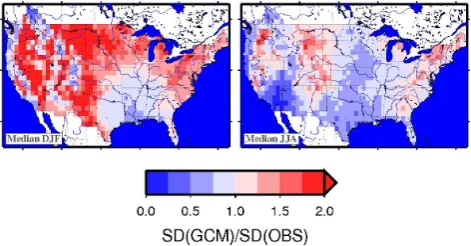
Fig. 3. Ensemble median of the ratio of the standard deviation (SD)
for the GCMs to the SD of the observations for daily precipitation during DJF and JJA for 1979–1993.
where the subscript x is either obs, raw or BC for obser-vations, raw AGCM, or bias corrected AGCM precipitation, and the overbar indicates a mean for the period. To quantify the effect of the BC on the precipitation change between the two periods, we used a trend modification index, TM, defined as
TM= |1Pbc−1Pobs| − |1Praw−1Pobs|,mm d−1, (2) where vertical bars are the absolute value. This index has the property of having values greater than 0 where the bias correction degrades the correspondence between the climate model and observed precipitation changes. Equation (2) em-phasizes that we examine changes in terms of differences rather than ratios (or fractions).
3 Results and discussion
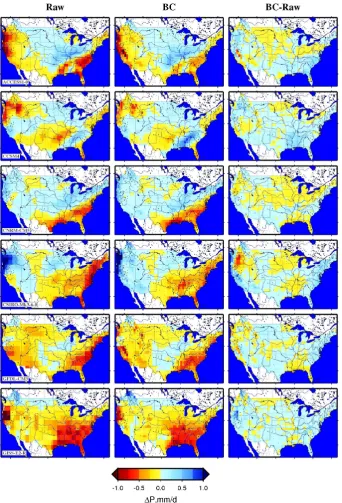
[image:3.595.310.546.228.351.2]Fig. 4. For GCMs 1–6, the change in mean DJF precipitation between 1979–1993 and 1994–2005 for the raw GCM output (left column) and
bias corrected GCM output (center); the difference between the two is in the right column.
bias (underestimate) in standard deviation. The future GCM projection assumes a 40 % increase in mean relative to the historic GCM. The arrows indicate what would happen dur-ing quantile mappdur-ing of the GCM’s raw future projection for two values corresponding to a low (20th percentile) and high (80th percentile) value. For the 80th percentile value, the fu-ture GCM value of 55.7 corresponds to a 95th percentile for the raw historic GCM data. The 95th percentile of the
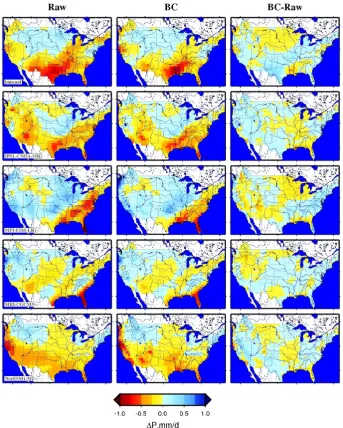
Fig. 5. Same as Fig. 4 but for GCMs 7-11.
observations. The original change at the 80th percentile is 15.6, and the post-BC change is 21.2; at the 20th percentile the original change is 7.4 and the post-BC change is 8.6.
Figure 2 continues with the synthetic data from Fig. 1, but presents probability distribution functions to illustrate more clearly the effect of the imposed bias in variance on the pro-jected change through the bias correction process. Figure 2a shows that the 40 % increase in the raw GCM data is am-plified to a 56 % increase by the QM process. If the syn-thetic distribution were symmetrical, a comparable decrease in GCM simulated mean would be amplified in the opposite direction, and if projected changes were negative as often as positive, then this amplifying effect would be offset and the quantile mapping would have little net effect on trends or shifts. However, because the distributions in Fig. 2a are
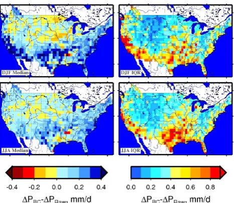
Fig. 6. Ensemble median difference between the BC and raw
dif-ferences in precipitation between 1994–2005 and 1979–1993 for DJF (top row) and JJA (bottom row). Right column is the interquar-tile range (IQR), defined as the 75th perceninterquar-tile minus the 25th per-centile.
The connection between bias correction, the variance, and the trend can be understood more clearly by analyzing a sim-ple change in the median. LetM0.5E be the model median in the early period, with the subscript 0.5 indicating the quan-tile (50th percenquan-tile or median) and the superscript E for the early period. The model median in the late period is then
M0.5L , and we are interested in the effect of bias correction on the model-predicted change in median,M0.5L −M0.5E . Will bias correction amplify or reduce this change? Assuming the change is nonzero, we can writeM0.5L =MpE, wherep6=0.5 is the percentile value of the new model median in the old model distribution. The raw model-projected change in me-dian is then simplyMpE−M0.5E . QM will map a model value with percentilep in the early period to the observed value at the same percentile: QM(MpE)=OpE, whereO indicates an observed value. The bias corrected change in median is therefore QM(MpE)−QM(M0.5E )=OpE−O0.5E . Since we have already stipulatedp6=0.5, we can compare the magnitude of the bias corrected to original change in median using a bias-correction ratio (BCR):
BCR= O
E p−O0.5E ME
p−M0.5E
. (3)
BCR<1 (bias correction reduces the model change) when the model difference between thepth percentile and median value is larger than the observed difference between thepth percentile and the median value – i.e., when the model has too much variance. Similarly, where BCR>1, bias correc-tion will increase the model change (when the model has less variance than observed). Furthermore, Eq. (3) indicates that
Fig. 7. Difference between observed seasonal mean precipitation of
1994–2005 and 1979–1993.
QM does not alter the sign of the model-predicted change (at least in this simple case) and that the alteration of the change is insensitive to any positive or negative bias between the model and observations, being affected only by the rela-tive variance of the two. From this simple synthetic demon-stration it can be inferred that, if there were a preponderance of GCMs with biases in variance in the same direction, the net effect of QM on the simulated difference between eras could be systematically in one direction, even with random biases in the mean.
In reality trends in non-normally distributed variables can-not be represented just by changes in the median, and GCMs exhibit much more complex biases than simply an overesti-mate or underestioveresti-mate of variance, with differing biases at different times, in different seasons, and at different quan-tiles, for example (Boberg and Christensen, 2012; Maurer et al., 2013; Themeßl et al., 2011), all of which can affect the modification of GCM simulated changes by QM. Thus, simply characterizing a GCM as exhibiting a certain bias in standard deviation will not exactly predict the effect of bias correction on trends. In any case, for illustration, Fig. 3 shows the ensemble median of biases in standard deviation, expressed as a ratio of simulated to observed standard devi-ation, for the 11 AGCMs included in this study for two sea-sons: DJF and JJA. This shows areas where there appears to be consistent underprediction of standard deviation by a ma-jority of AGCMs, such as in the southeastern portion of the domain. This means there may be a potential for the trends in the raw output from many of the AGCMs to be modified by the bias correction process.
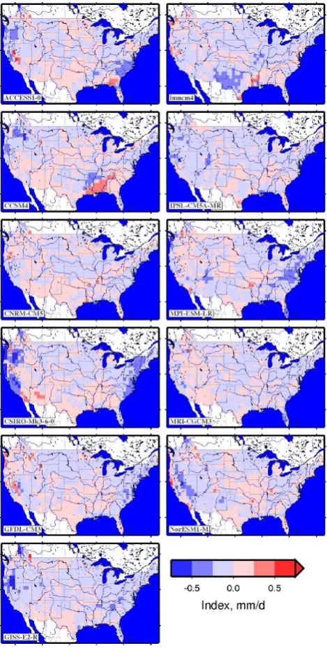
[image:6.595.309.547.64.198.2]Fig. 8. For DJF, the TM index (described in the text) values for each
GCM.
produces a wettening or drying effect for each AGCM, there is considerable variation among the AGCMs.
While not shown here, for JJA precipitation the changes due to the BC process for each AGCM appear slightly less prominent than for DJF relative to the raw AGCM precipi-tation changes between the two periods. Figure 6 shows the ensemble median change and the interquartile range (IQR) between the BC and raw precipitation differences for the two periods for both DJF and JJA. The left column represents the ensemble median effect of BC on the seasonal mean precip-itation difference between 1994–2005 and 1979–1993. The
IQR in Fig. 6 is analogous to the standard deviation, repre-senting the spread of the AGCMs about the median. In gen-eral, where the ensemble median has the greatest magnitude, the IQR is also large, indicating high variability among the models in the effect of BC on the precipitation change. The changes in precipitation differences induced by the BC pro-cess in Fig. 6 can be a cause for concern. While in large portions of the domain they are small in comparison to the observed difference in mean precipitation between the two periods (Fig. 7), at many individual points the effect can be substantial. For example, for the DJF median panel in Fig. 6, there is a swath of dark blue grid cells along the southern west coast, with a median effect of the BC on the precipita-tion trend of 0.4 mm d−1 or higher. This would be an im-portant modification based on the observed differences in Fig. 7, with a median change between the periods of 0.5– 1.0 mm d−1. Second, the DJF IQR for these cells is greater
than 0.5 mm d−1, indicating that 25 % of the AGCMs would
show trend modifications by BC in excess of approximately 0.65 mm d−1(the median plus half of the IQR), which is on the order of the observed trend in Fig. 7. This latter point makes clear the importance in using an ensemble of climate models rather than one or a few, since the regions of en-hancement/reduction of trends are not coherent across dif-ferent models and the effect diminishes when combined into an ensemble.
Perhaps more importantly, in Fig. 6, some areas where the BC process appears (in the median) to produce much wet-ter conditions than the raw AGCM are also areas where the observed difference between the 1994–2005 and 1979–1993 periods is considerably higher than the AGCMs simulate. One example is the Pacific northwest, where Figs. 4 and 5 show more than half the models simulating drying DJF ditions between 1994–2005 and 1979–1993, in distinct con-trast to the wettening trend in the observations (Fig. 7). It should be emphasized that the BC only adjusts the quantiles of the AGCM to match those of observations within a 15 yr training period – there is no attempt to match trends, either within the 15 yr training period or over longer periods. Thus, any trends are inherited directly from the AGCM, though the QM can, as discussed above, modify these.
Fig. 9. For DJF and JJA, the ensemble median TM index value (left panels), the locations of grid cells (dark rectangles) where the 25th
percentile TM index value exceeds 0 (center panels), and the grid cells where the 75th percentile value is less than 0.
areas of improved and degraded precipitation trend represen-tation due to BC. Regions with improved or degraded skill vary from model to model, with no apparent geographical consistency. In sum, the errors in an individual model’s vari-ance appear unrelated to the errors in the model’s trend.
Figure 9 summarizes the results for the ensemble in Fig. 8 and the similar ensemble for JJA. The median TM values (left panels) tend to lie close to zero, and neither degraded (TM>0) nor improved (TM<0) values dominate the pic-ture for either DJF or JJA. The center panels highlight re-gions where 75 % of the AGCMs show a degraded change in precipitation (relative to the observed change) due to the BC process. These cases constitute 4.3 % of the grid cells for DJF and 13.0 % of the grid cells for JJA. The right panels show the grid cells where 75 % of the AGCMs show improved cor-respondence with the observed change after BC. These cover 26.2 and 4.5 % of the domain for DJF and JJA, respectively.
This suggests that with an ensemble of 11 AGCMs as used in this effort the BC produces no consistent improve-ment or degradation in the simulated AGCM precipitation change. While the effect of BC on the trend can be signifi-cant, it tends as often as not to bring AGCM simulated trends closer to observed trends for the periods used in this study. However, there are isolated locations where the trend appears to be degraded for most model simulations, which could be of particular interest for impacts studies. One such case is the southwestern portion of the domain, where Fig. 9 (cen-ter panels) shows the grid cells for which JJA precipitation trends are degraded for 75 % of the AGCM simulations by the BC process. For these locations, it may be beneficial to retain the raw GCM simulated trend during impacts analysis studies. Conversely, in Fig. 9 (right panels) there are many grid cells in the northeast where DJF precipitation trends are improved by BC for most of the AGCM simulations.
One of the driving motivations for much downscaling is the investigation of regional and local hydrological impacts of climate change (Fowler et al., 2007). Since the runoff re-sponse to changing precipitation is highly nonlinear (Wigley and Jones, 1985), changes in precipitation are amplified in their convolution to runoff changes. This emphasizes the im-portance in ensuring that the projected precipitation trends not be degraded during the BC process, since the implica-tions would be for even greater biases in projected runoff changes.
4 Summary and conclusions
Quantile mapping bias correction has been shown to mod-ify the projected changes, or trends, produced by climate models. This is of critical concern regarding precipitation projections, where changes to the raw climate model output can have significant impacts on the implications for water supply and management in the face of climate change. The resulting discrepancy between the raw climate model out-put and bias corrected outout-put leaves some ambiguity as to whether the bias correction should be modified to preserve the original climate model simulated changes. It is empha-sized that this study is only concerned with the effect of quantile mapping on precipitation trends. It includes no as-sessment of the effectiveness of quantile mapping at reducing biases, which would be enhanced by considering the differ-ent sources of bias.
were compared between precipitation for two periods, 1979–1993 and 1994–2005 for all AGCMs, both before and after a quantile mapping bias correction, and grid-ded observed precipitation. We consider winter and summer precipitation separately.
We found that the bias correction did produce differ-ent precipitation changes from the raw AGCM output, with a wettening effect in some locations and a drying effect in others. While there was some spatial consistency in re-gions showing a tendency for bias correction to make the projections wetter or drier, the skill, measured as a corre-spondence to observed changes, was more variable, with different AGCMs responding to bias correction differently. Taken as an ensemble, the bias correction had no coherent, overwhelming negative or positive effect on the correspon-dence of the simulated to observed precipitation changes between periods. Reliance on a single AGCM or a small sample of AGCMs however could, for some regions, re-sult in a degraded simulated trend in precipitation due to bias correction.
Based on these results, it does not appear that there is a clear advantage to either preserving the raw AGCM simu-lated trend in precipitation during bias correction or allowing the trend to be modified by the process. In most locations, as long as a reasonable ensemble size is used, even though the trend in seasonal precipitation may be modified in the pro-cess, it may be as likely as not to be beneficial to do so. Sim-ilar to the suggestions by others (Cloke et al., 2013), it may be prudent for practitioners to examine the projected trends in raw AGCM output as well as in bias corrected output, to be completely transparent as to the effects of bias correction on trends.
[image:9.595.317.539.74.509.2]These findings are limited to the extent of this study, namely seasonal mean precipitation for the observed periods used here. This focus was motivated by the observation of changes in trends in mean precipitation produced by quantile mapping. Since changes in the magnitude of extreme pre-cipitation events are important for assessing many impacts to society, future efforts will examine the effect of quantile mapping bias correction on trends in extreme events. Quan-tile mapping can have different effects at the tails of distri-butions (Li et al., 2010), and changes in the projected trends in extreme events due to quantile mapping have not been ex-plored. Furthermore, the bias correction was performed at a 1◦ spatial scale, so that the observations are comparable to the scale of the climate models. At finer scales, the biases between interpolated AGCM output and observations would be expected to be much more heterogeneous, and the impact of quantile mapping bias correction at finer scales could be quite different from that found here, though employing quan-tile mapping to downscale to fine scales has been found to be problematic (Maraun, 2013).
Table A1. Climate models used in this study.
Modeling center Model name 1 Commonwealth Scientific and
Industrial Research Organiza-tion (CSIRO) and Bureau of Meteorology (BOM), Australia
ACCESS1.0
2 National Center for Atmospheric Research
CCSM4
3 Centre National de Recherches
Météorologiques/Centre Européen de Recherche et Formation Avancée en Calcul Scientifique
CNRM-CM5
4 Commonwealth Scientific and Industrial Research Organi-zation in collaboration with Queensland Climate Change Centre of Excellence
CSIRO-Mk3.6.0
5 NOAA Geophysical Fluid Dynamics Laboratory
GFDL-CM3
6 NASA Goddard Institute for Space Studies
GISS-E2-R
7 Institute for Numerical Mathematics
INM-CM4
8 Institut Pierre-Simon Laplace IPSL-CM5A-MR 9 Max-Planck-Institut für
Mete-orologie (Max Planck Institute for Meteorology)
MPI-ESM-LR
10 Meteorological Research Institute
MRI-CGCM3
11 Norwegian Climate Centre NorESM1-M
Acknowledgements. This research was supported in part by the
California Energy Commission Public Interest Energy Research (PIER) Program. We acknowledge the World Climate Research Programme’s Working Group on Coupled Modelling, which is responsible for CMIP, and we thank the climate modeling groups (listed in Table A1 of this paper) for producing and making available their model output. For CMIP the US Department of En-ergy’s Program for Climate Model Diagnosis and Intercomparison provided coordinating support and led development of software infrastructure in partnership with the Global Organization for Earth System Science Portals.
References
Barsugli, J. J.: What’s a billion cubic meters among friends: The impacts of quantile mapping bias correction on climate projec-tions, 2010 Fall Meeting, American Geophysical Union, San Francisco, CA, 13–17 December 2010, 2010.
Boberg, F. and Christensen, J. H.: Overestimation of Mediterranean summer temperature projections due to model deficiencies, Nat. Clim. Change, 2, 433–436, doi:10.1038/nclimate1454, 2012. Brekke, L., Thrasher, B., Maurer, E. P., and Pruitt, T.: Downscaled
CMIP3 and CMIP5 Climate Projections: Release of Downscaled CMIP5 Climate Projections, Comparison with Preceding Infor-mation, and Summary of User Needs, US Dept. of Interior, Bu-reau of Reclamation, Denver, CO, 104 pp., 2013.
Christensen, J. H., Hewitson, B., Busuioc, A., Chen, A., Gao, X., Held, I., Jones, R., Kolli, R. K., Kwon, W.-T., Laprise, R., Mag-aña Rueda, V., Mearns, L., Menéndez, C. G., Räisänen, J., Rinke, A., Sarr, A., and Whetton, P.: Regional climate projections, in: Climate Change 2007: The Physical Science Basis. Contribution of Working Group I to the Fourth Assessment Report of the In-tergovernmental Panel on Climate Change edited by: Solomon, S., Qin, D., Manning, M., Chen, Z., Marquis, M., Averyt, K. B., Tignor, M., and Miller, H. L., Cambridge University Press, Cam-bridge, United Kingdom and New York, NY, USA, 2007. Cloke, H. L., Wetterhall, F., He, Y., Freer, J. E., and
Pappen-berger, F.: Modelling climate impact on floods with ensemble climate projections, Q. J. Roy. Meteorol. Soc., 139, 282–297, doi:10.1002/qj.1998, 2013.
Deser, C., Knutti, R., Solomon, S., and Phillips, A. S.: Communi-cation of the role of natural variability in future North American climate, Nat. Clim. Change, 2, 775–779, 2012.
Dobler, C., Hagemann, S., Wilby, R. L., and Stötter, J.: Quantify-ing different sources of uncertainty in hydrological projections in an Alpine watershed, Hydrol. Earth Syst. Sci., 16, 4343–4360, doi:10.5194/hess-16-4343-2012, 2012.
Eden, J. M., Widmann, M., Grawe, D., and Rast, S.: Skill, Correc-tion, and Downscaling of GCM-Simulated PrecipitaCorrec-tion, J. Cli-mate, 25, 3970–3984, doi:10.1175/jcli-d-11-00254.1, 2012. Fowler, H. J., Blenkinsop, S., and Tebaldi, C.: Linking climate
change modelling to impacts studies: recent advances in down-scaling techniques for hydrological modelling, Int. J. Climatol., 27, 1547–1578, doi:1510.1002/joc.1556, 2007.
Girvetz, E. H., Zganjar, C., Raber, G. T., Maurer, E. P., Kareiva, P., and Lawler, J. J.: Applied Climate-Change Anal-ysis: The Climate Wizard Tool, PLoS ONE, 4, e8320, doi:10.1371/journal.pone.0008320, 2009.
Glahn, H. R. and Lowry, D. A.: The use of model output statistics (MOS) in objective weather forecasting, J. Appl. Meteorol., 11, 1203–1211, 1972.
Gudmundsson, L., Bremnes, J. B., Haugen, J. E., and Engen-Skaugen, T.: Technical Note: Downscaling RCM precipitation to the station scale using statistical transformations – a com-parison of methods, Hydrol. Earth Syst. Sci., 16, 3383–3390, doi:10.5194/hess-16-3383-2012, 2012.
Hagemann, S., Chen, C., Haerter, J. O., Heinke, J., Gerten, D., and Piani, C.: Impact of a Statistical Bias Correction on the Projected Hydrological Changes Obtained from Three GCMs and Two Hydrology Models, J. Hydrometeorol., 12, 556–578, doi:10.1175/2011jhm1336.1, 2011.
Hawkins, E. and Sutton, R.: The potential to narrow uncertainty in projections of regional precipitation change, Clim. Dynam., 37, 407–418, doi:10.1007/s00382-010-0810-6, 2011.
Hoerling, M., Eischeid, J., and Perlwitz, J.: Regional Precipitation Trends: Distinguishing Natural Variability from Anthropogenic Forcing, J. Climate, 23, 2131–2145, doi:10.1175/2009jcli3420.1, 2010.
Li, H., Sheffield, J., and Wood, E. F.: Bias correction of monthly precipitation and temperature fields from Intergovern-mental Panel on Climate Change AR4 models using equidis-tant quantile matching, J. Geophys. Res., 115, D10101, doi:10.1029/2009jd012882, 2010.
Livneh, B., Rosenberg, E. A., Lin, C., Nijssen, B., Mishra, V., An-dreadis, K. M., Maurer, E. P., and Lettenmaier, D. P.: A Long-Term Hydrologically Based Dataset of Land Surface Fluxes and States for the Conterminous United States: Update and Extensions*, J. Climate, 26, 9384–9392, doi:10.1175/jcli-d-12-00508.1, 2013.
Maraun, D., Wetterhall, F., Ireson, A. M., Chandler, R. E., Kendon, E. J., Widmann, M., Brienen, S., Rust, H. W., Sauter, T., The-meßl, M., Venema, V. K. C., Chun, K. P., Goodess, C. M., Jones, R. G., Onof, C., Vrac, M., and Thiele-Eich, I.: Precipi-tation downscaling under climate change: Recent developments to bridge the gap between dynamical models and the end user, Rev. Geophys., 48, RG3003, doi:10.1029/2009rg000314, 2010. Maraun, D.: Nonstationarities of regional climate model biases in
European seasonal mean temperature and precipitation sums, Geophys. Res. Lett., 39, L06706, doi:10.1029/2012gl051210, 2012.
Maraun, D.: Bias Correction, Quantile Mapping, and Downscal-ing: Revisiting the Inflation Issue, J. Climate, 26, 2137–2143, doi:10.1175/jcli-d-12-00821.1, 2013.
Maurer, E. P., Hidalgo, H. G., Das, T., Dettinger, M. D., and Cayan, D. R.: The utility of daily large-scale climate data in the assessment of climate change impacts on daily stream-flow in California, Hydrol. Earth System Sci., 14, 1125–1138, doi:1110.5194/hess-1114-1125-2010, 2010.
Maurer, E. P., Das, T., and Cayan, D. R.: Errors in climate model daily precipitation and temperature output: time invariance and implications for bias correction, Hydrol. Earth Syst. Sci., 17, 2147–2159, doi:10.5194/hess-17-2147-2013, 2013.
Maurer, E. P., Brekke, L., Pruitt, T., Thrasher, B., Long, J., Duffy, P. B., Dettinger, M. D., Cayan, D., and Arnold, J.: An enhanced archive facilitating climate impacts analysis, B. Am. Meteorol. Soc., doi:10.1175/bams-d-13-00126.1, in press, 2014.
Murphy, J.: An evaluation of statistical and dynamical techniques for downscaling local climate, J. Climate, 12, 2256–2284, 1999. Panofsky, H. A. and Brier, G. W.: Some Applications of Statistics to Meteorology, The Pennsylvania State University, University Park, PA, USA, 224 pp., 1968.
Piani, C., Haerter, J., and Coppola, E.: Statistical bias correction for daily precipitation in regional climate models over Europe, Theor. Appl. Climatol., 99, 187–192, doi:10.1007/s00704-009-0134-9, 2010.
precipitation changes in California, J. Climate, 26, 5879–5896, doi:10.1175/jcli-d-12-00766.1, 2013.
Taylor, K. E., Stouffer, R. J., and Meehl, G. A.: An Overview of CMIP5 and the experiment design, B. Am. Meteorol. Soc., 93, 485–498, doi:410.1175/BAMS-D-1111-00094.00091, 2012. Themeßl, M., Gobiet, A., and Leuprecht, A.: Empirical-statistical
downscaling and error correction of daily precipitation from regional climate models, Int. J. Climatol., 31, 1530–1544, doi:10.1002/joc.2168, 2011.
Thrasher, B., Maurer, E. P., McKellar, C., and Duffy, P. B.: Techni-cal Note: Bias correcting climate model simulated daily temper-ature extremes with quantile mapping, Hydrol. Earth Syst. Sci., 16, 3309–3314, doi:10.5194/hess-3316-3309-2012, 2012.
Wigley, T. M. L. and Jones, P. D.: Influences of precipitation changes and direct CO2effects on streamflow, Nature, 314, 149–
152, 1985.
Wilks, D. S.: Rainfall Intensity, the Weibull Distribution, and Esti-mation of Daily Surface Runoff, J. Appl. Meteorol., 28, 52–58, doi:10.1175/1520-0450(1989)028<0052:ritwda>2.0.co;2, 1989. Wood, A. W., Leung, L. R., Sridhar, V., and Lettenmaier, D. P.: