Munich Personal RePEc Archive
GMM Estimation with Noncausal
Instruments
Lanne, Markku and Saikkonen, Pentti
University of Helsinki, HECER
September 2009
Online at
https://mpra.ub.uni-muenchen.de/23649/
öMmföäflsäafaäsflassflassflas ffffffffffffffffffffffffffffffffffff
Discussion Papers
GMM Estimation with Noncausal Instruments
Markku Lanne
University of Helsinki, RUESG and HECER
and
Pentti Saikkonen
University of Helsinki, RUESG and HECER
Discussion Paper No. 274 September 2009
ISSN 1795-0562
HECER
Discussion Paper No. 274
GMM Estimation with Noncausal Instruments*
Abstract
Lagged variables are often used as instruments when the generalized method of moments (GMM) is applied to time series data. We show that if these variables follow noncausal autoregressive processes, their lags are not valid instruments and the GMM estimator is inconsistent. Moreover, in this case, endogeneity of the instruments may not be revealed by the J-test of overidentifying restrictions that may be inconsistent and, as shown by simulations, its finite-sample power is, in general, low. Although our explicit results pertain to a simple linear regression, they can be easily generalized. Our empirical results indicate that noncausality is quite common among economic variables, making these problems highly relevant.
JEL Classification: C12, C22, C51
Keywords: Noncausal autoregression, instrumental variables, test of overidentifying restrictions
Markku Lanne Pentti Saikkonen
Department of Economics, Department of Mathematics and Statistics P.O. Box 17 (Arkadiankatu 7) P.O. Box 68 (Gustaf Hällströmn katu 2b) FI-00014 University of Helsinki FI-00014 University of Helsinki
FINLAND FINLAND
e-mail: [email protected] e-mail: [email protected]
1 Introduction
The generalized method of moments (GMM) is widely used in di¤erent …elds of
eco-nomics, including macroeconomics and …nance. Among other things, its popularity
presumably follows from the development of more and more complicated theoretical
models which would in practice be impossible to take to data by alternative
meth-ods, such as the method of maximum likelihdood (ML). Even if ML estimation were
possible, the GMM may be considered more robust in that it allows the researcher to
concentrate on the central implications of the theory without the need to specify an
empirical model in detail. In their survey, Hansen and West (2002) list the three most
common uses of the GMM in economics: estimation of a …rst-order condition or a
decision rule from dynamic optimization problem, examination of forecasting ability
of survey data or of a …nancial variable, and setups with e¢ciency gains from the use
of many moments. The …rst two of these are ubiquitous in the empirical analysis of
asset pricing models, while all of them pertain to macroeconomic applications.
For instrumental variable methods to be applicable, a su¢ciently large number of
instruments are needed that satisfy the relevance and exogeneity requirements. The
former has received more attention in the burgeoning weak instrument literature (see,
e.g., Stock, Wright and Yogo, 2002), while it has been thought that the exogeneity
of candidate instruments can reliably be determined by tests such as Hansen’s (1982)
J-test of overidentifying restrictions. Moreover, in applications using time series data,
lagged values of economic variables, especially those included in the model, have been
considered natural instruments that should be predetermined by construction.
Pro-vided the dynamics of such instruments can be described by causal autoregressive
(AR) processes, the exogeneity requirement is indeed satis…ed. However, while
eco-nomic variables typically can be adequately modeled as AR processes, noncausality
seems to be quite common among them (see Section 2.3) and, as we argue in this
paper, in that case lags are not, in general, valid instruments. The di¤erence between
past, whereas a noncausal AR process allows for dependence on the future.
Our theoretical (asymptotic) results pertain to the simple special case of univariate
linear regression with a conditionally homoskedastic error term. In addition, we
report results on simulation experiments to illustrate the …nite-sample behavior of the
GMM estimator and the J-test in the presence of noncausal instruments. The GMM
estimator is shown to be inconsistent in our simple setup, and the simulations show
that the biases of the ordinary least squares (OLS) estimator and the GMM estimator
are very close to each other, especially in the case where the instruments follow purely
noncausal AR processes. We also show that Hansen’s J-test can be inconsistent in
some cases and, therefore, futile in checking the exogeneity of the instruments when
noncausality is present. Even in cases where the test is not inconsistent, it may have
low …nite-sample power, as suggested by our simulation results. Although our …ndings
explicitly concern relatively simple special cases, it is easy to see that lagged values
of variables following noncausal AR processes are, in general, never valid instuments.
The plan of the paper is as follows. In Section 2, the noncausal AR process is
in-troduced and checking for its presence is discussed. In Subsection 2.3, we also present
evidence that economic time series are quite often better described as noncausal than
causal AR processes. Section 3 contains our main results concerning the asymptotic
and …nite-sample properties of the GMM estimator and the J-test. Finally, Section
4 concludes.
2 Noncausal autoregression
In this section, we brie‡y discuss noncausal AR processes as a prelude to the results
concerning the GMM estimation in Section 3. In addition to presenting one
parame-trization of the noncausal autoregression to be used throughout the paper, we pick
up on various aspects of model selection. Finally, we show evidence based on an
ex-tensive data set consisting of 343 macroeconomic and …nancial time series in favor of
put forth in this paper.
2.1 Model
The literature on noncausal AR models is not voluminous, and their economic
appli-cations are almost nonexistent. For a brief survey covering most of this literature,
see Lanne and Saikkonen (2008), who introduced a new formulation of the model,
developed the related likelihood-based theory of estimation and statistical inference,
and devised a model selection procedure. In particular, they considered a stochastic
process xt (t= 0; 1; 2; :::)generated by
' B 1
(B)xt= t; (1)
where (B) = 1 1B rBr,'(B
1
) = 1 '1B
1
'sB s, and tis a
sequence of independent, identically distributed (continuous) random variables with
mean zero and variance 2
or, brie‡y, t i:i:d:(0;
2
). Moreover, B is the usual
backward shift operator, that is, Bky
t = yt k (k = 0; 1; :::), and the polynomials
(z) and '(z) have their zeros outside the unit circle so that
(z)6= 0 for jzj 1 and '(z)6= 0 for jzj 1: (2)
We use the abbreviation AR(r; s) for the model de…ned by (1) and sometimes
write AR(r) for AR(r;0). If'1 = ='s= 0, model (1) reduces to the conventional
causal AR(r) process with yt depending on its past but not future values. The more
interesting cases from the viewpoint of this paper arise, when this restriction does
not hold. If 1 = = r = 0, we have the purely noncausal AR(0; s) model with
dependence on future values only. In the mixed AR(r; s) case where neither restriction
holds, yt depends on its past as well as future values. Our simulation results suggest
that the problems due to the endogeneity of the instruments are severest when the
instruments follow a purely noncausal AR process, but they can be substantial also
in the case of a mixed process. However, to some extent these problems are mitigated
The conditions in (2) imply that xt has the two-sided moving average
representa-tion
xt = 1
X
j= 1
j t j; (3)
where j is the coe¢cient ofzj in the Laurent series expansion of (z)
1
'(z 1
) 1 def=
(z). This expansion exists in some annulus b <jzj< b 1
with 0 < b <1 and with
jjj converging to zero exponentially fast as jjj ! 1. It is well-known that xt also
has a causal AR(p) representation withp=r+s and the autoregressive polynomial
given bya(B) = 1 a1B apBp ='(B) (B)(see Brockwell and Davis (1987,
p. 124–125) and Lanne and Saikkonen (2009)). Thus, we can write
a(B)xt= t; (4)
where the (stationary) error term t is uncorrelated but, in general, not independent
with mean zero and variance 2
.
2.2 Checking for noncausality
It is well-known that causal and noncausal AR processes cannot be distinguished by
autocorrelation functions. This means that they are not identi…ed by Gaussian
like-lihood, so non-Gaussian distributions must be considered in ML estimation.
There-fore, the …rst step in modeling a potentially noncausal time series is to search for
signs of nonnormality. To this end, Lanne and Saikkonen (2008) suggest estimating
an adequate Gaussian AR(p) model and checking its residuals for nonnormality. For
economic and …nancial time series, the residuals are often leptokurtic, indicating that
Student’s t-distribution might be suitable. In their application to the U.S. in‡ation
series as well as for a large number of series discussed below, this indeed seems to be
the case.
Once nonnormality has been established, the next step is to select among the
alternative AR(r; s) speci…cations. As the AR(p) model has been found to adequately
models with r+s =p. Following Breidt et al. (1991), Lanne and Saikkonen (2008)
suggested selecting among these the model that produces the greatest value of the
likelihood function. Finally, the adequacy of the selected speci…cation is checked
diagnostically and the model is augmented if needed. In addition to examining the …t
of thet-distribution, Lanne and Saikkonen (2008) checked the residuals for remaining
autocorrelation and conditional heteroskedasticity.
The purpose of …tting a Gaussian AR model in the …rst step is only to help
in determining the correct lag length and checking for nonnormality. Sometimes it
may not be possible to come up with a satisfactory Gaussian AR model, in which
case an adequate model might still be found among di¤erent non-Gaussian AR(r; s)
speci…cations.
2.3 Prevalence of noncausality
In order to assess the signi…cance of the problems caused by noncausal instruments
in practice, we checked a large number of macroeconomic and …nancial variables
for noncausality using the algorithm discussed in Subsection 2.2. In particular, we
considered 343 time series from the seven-country data set of Stock and Watson
(2004).1
Using a Gaussian likelihood, we were able to …nd a causal AR model adequate
in the sense of capturing all autocorrelation for 260 of the considered series. In 202
cases, it is a noncausal speci…cation that maximizes the likelihood function, and 136
of the selected models satisfy the diagnostic checks mentioned in Subsection 2.2 at
1This data set contains various asset prices, measures of activity (such as the real GDP,
unem-ployment and consumer price index), wages, commodity prices, and money measures from Canada,
France, Germany, Italy, Japan, UK and US. The data are monthly or quarterly and for the most
part cover the years 1959–1999 although some series are available only for a shorter period. For
most series we used various transformations, such as logs or di¤erences, and we consider these as
di¤erent time series in counting the total number of series. For details on the data, see Stock and
the 5% level. In the remaining cases, there were signs of some unmodeled conditional
heteroskedasticity and fat tails not satisfactorily captured by the t-distribution. Of
the 83 series for which an adequate causal AR model could not be found as a starting
point, in 40 cases a noncausal AR model turned out to be diagnostically satisfactory
such that this model also maximizes the likelihood function among all AR
speci…ca-tions of the same order. All in all, we then have quite strong evidence in favor of
noncausality in economic time series: of the 343 time series considered, 300 series
show clear signs of noncausality and for 176 series an adequate noncausal AR model
can be speci…ed. These …ndings indicate that the possibility of noncausality should
be kept in mind when using instrumental variables methods.
To take an example from the empirical literature employing the GMM estimator,
we checked the instruments used by Campbell and Mankiw (1990) for noncausality.
These authors tested the permanent income hypothesis by testing for the signi…cance
of the slope coe¢cient in a regression of the change in US aggregate consumption
on the change in disposable income (quarterly data from 1953:1 to 1985:4). whether
the slope coe¢cient equals zero. As instruments they used lagged di¤erences of
ag-gregate consumption, disposable income and interest rates, in various combinations.
By the algorithm discussed in Section 2.2, all of these variables can be described as
noncausal AR processes. Therefore, as will be explained in Section 3 below, it is not
suprising that their two-stage least squares (2SLS) estimates do not di¤er much from
the OLS estimate. Moreover, the test of overidentifying restrictions failed to reject
at conventional signi…cance levels for any combination of the instruments.
3 GMM with noncausal instruments
3.1 Model
In order to illustrate our main points we consider the simple time series regression
model.
where the error term "1t is independent and identically distributed (i:i:d:) with zero
mean. Despite its simplicity, this model serves to make our main points, and, as a
matter of fact, even this simple regression model has been used quite frequently in
empirical analysis. Typical examples include testing the permanent income hypothesis
(e.g., Campbell and Mankiw, 1990) and consumption-based asset pricing models (see,
Campbell et al. (1997, 311–313, and the references therein). The regressor xt is
supposed to follow the noncausal autoregression (1), rewritten here for convenience,
' B 1
(B)xt="2t; (6)
where"2t is a zero meani:i:d:error term. Because we are interested in the case where
the regressor and error term in (5) are correlated we let"t= ["1t "2t]0be a generali:i:d:
error vector. Thus, de…ning the covariance matrix = [ ij]i;j=1;2 with ii = 2
i we
assume"t i:i:d:(0; )where, unless otherwise stated, 12is nonzero. For simplicity,
we have omitted intercept terms from (5) and (6). Their inclusion would only mean
using mean corrected data and, by standard arguments, it can be seen that mean
correction has no e¤ect on our asymptotic derivations. In our simulations intercept
terms are included, however.
3.2 GMM estimation
When regressors are correlated with the error term, OLS estimation is inconsistent,
and, therefore, GMM estimation is typically employed. That correlation between
the regressor and error term results in (5) can be seen from (3) and the assumption
12 6= 0. In a case like this it is quite common to use lagged values of the regressor
as instruments in GMM estimation. However, in the noncausal case these are not
valid instruments. This is immediately seen by using (3) to obtain Cor(xt i; "1t) =
E(xt i; "1t) = 12 i, i > 0, where i is generally nonzero when the regressor is
noncausal. One might think that in practice an application of the standard J-test
(see Hansen, 1982) would reveal the problem. However, the J-test is known to have
this can actually happen when noncausal instruments are employed.
Our subsequent derivations assume that the vector of instruments is given by
zt 1 = [xt 1 xt p]0. At the end of this section we discus how to modify the results
when other choices of instruments are employed. Note that using p lagged values
of the regressor as instruments is appropriate because the regressor has a causal
AR(p) representation (see (4)). Given this, and the fact that the errors in (5) are
i:i:d:, means that our results indicate how badly things can go wrong even in a fairly
favorable situation.
In our simple set up the GMM estimation boils down to classical 2SLS estimation.
Suppose we have data fort= p+ 1; :::;0;1; :::; T with the …rst pobservations of the
regressor used as initial values in the LS estimation of the parametersa1; :::; ap in (4).
It will be convenient to introduce the parameter vector a = [a1 ap]0. The 2SLS
estimator is de…ned as
~ =
T
X
t=1
^
xtxt
! 1
T
X
t=1
^
xtyt;
where x^t= ^a0zt 1 with
^
a=
T
X
t=1
zt 1zt0 1
! 1
T
X
t=1
zt 1xt;
the OLS estimator of a. The inconsistency of ~ in the noncausal case was already
made clear but we nevertheless derive its probability limit, as the result is needed
later.
Stationarity and standard arguments show that^a!p E zt 1zt0 1 1
E(zt 1xt) =
a and, furthermore,
~ = + a^0T 1
T
X
t=1
zt 1xt
! 1
^
a0T 1
T
X
t=1
zt 1"1t
p
! + (a0E(zt 1xt)) 1
a0E(zt 1"1t):
Let k =E(xt kxt) be the autocovariance function of xt and k = k= 0 the
corre-sponding autocorrelation function. Then, if = 1 p
0
and = 1 p
we can write E(zt 1xt) = 0 and, using (3), E(zt 1"1t) = 12 . With this notation
the preceding result reads as
~ p
! + 12a
0
0a0
: (7)
Thus, the 2SLS estimator is inconsistent when the numerator of the latter term on
the right hand side is nonzero.
Now consider theJ-test which is based on the covariance between the instruments
and the 2SLS residual ~"1t =yt ~xt (t= 1; :::; T). The test statistic or in this case
Sargan’s statistic can be written as
J = T ~2 1 T 1 T X t=1
zt 1~"1t
!0
T 1
T
X
t=1
zt 1zt0 1
! 1
T 1
T
X
t=1
zt 1~"1t
!
; (8)
where ~2 1 =T
1PT
t=1~" 2
1t. The test assumes that the number of instruments is larger
than the number of regressors or, in our case, that p >1. In practice one applies the
test by comparing the observed value ofJ to quantiles of the 2
p 1 distribution.
On the right hand side of (8) we have
T 1
T
X
t=1
zt 1~"1t=T 1
T
X
t=1
zt 1"1t (~ )T 1
T
X
t=1
zt 1xt;
and, furthermore, (see (7) and the derivations preceding it)
T 1
T
X
t=1
zt 1~"1t p
! 12
12a0
a0 : (9)
The limit on the right hand side is zero when 12 is zero. Then the regressor is
strictly exogenous, which is not the case of our interest. However, the limit in (9)
can also be zero when 12 is nonzero. This happens when = c for some nonzero
real number c. This in turn happens in the purely noncausal case where r = 0 in (6)
(and s = p) if only one of the parameters '1; :::; 'p is nonzero. To see this, suppose
that, for example, '1 6= 0 and '2 = = 'p = 0. Then we also have 'i = ai
(i= 1; :::; p)and from (3) and (4) it follows that j =' j
1 = j (j 1). Thus, = ,
case the probability limit of the OLS estimator of is + 12= 0, and a comparison
with (7) reveals that this equals the probability limit of the 2SLS estimator. Thus,
in this special case, the 2SLS estimator can be expected to be equally biased as the
OLS estimator. Our simulation results con…rm this and show that the bias of the
2SLS can be substantial also in other cases.
When the right hand side of (9) is zero, arguments similar to those already used
show that J = Op(1), implying that the J-test is inconsistent. Thus, one might
suspect that the power of theJ-test is poor also when the limit in (9) is nonzero but
‘small’. According to our simulations this indeed seems to be the case.
The preceding derivations can straightforwardly be modi…ed to the case of general
instruments. To illustrate this, de…ne the noncausal AR(r; s) process wt by
substi-tutingwt forxt in (6). Then (3) and (4) also hold withwtin place of xt and de…ning
zt 1 = [wt 1 wt p]0 the previous expressions for the OLS estimator^aand its
prob-ability limit a apply. Furthermore, (7) holds with the ith component of the vector
0 given by Cov(wt i; xt) (i= 1; :::; p) whereas is as before except that its
com-ponents are obtained from (3) with wt in place of xt. It follows that (9) holds with
as de…ned above and the ith component of the vector given by Cor(wt i; xt),
the cross correlation betweenwt iand xt(i= 1; :::; p). The condition where the right
hand side of (9) becomes zero is as before but giving concrete examples of this is more
di¢cult than in the case where the instruments are lags of the regressor.
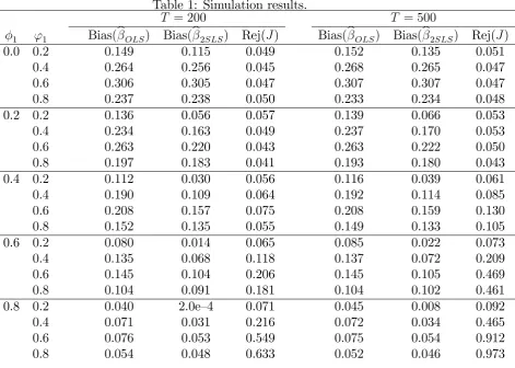
3.3 Simulation results
In this section, we report results of some simulation experiments to demonstrate the
relevance of the asymptotic results of Section 3.2 in …nite samples. Speci…cally, we
simulate 10,000 realizations from model (5)–(6) with r+s = 2 using a number of
combinations of '1 and 1. In all experiments, = 1:0 and also an intercept, whose
true value equals zero, is estimated. The errors are drawn from a bivariate normal
distribution with 2 1 =
2
not a¤ected by the values of these parameters. From each simulated bivariate time
series, the parameters of the simple regression model are estimated by both OLS and
2SLS, and the value of theJ-test statistic is computed. We consider two sample sizes,
200 and 500, but the results do not seem to be much a¤ected by the length of the
simulated realization.
In Table 1 we present a subset of our simulation results to highlight the main
…ndings. The biases of the OLS and 2SLS estimates are reported as averages over
all replications and the rejection rate of the J-test with nominal size 5%. Let us
…rst consider the cases in the uppermost panel, where the instruments follow a purely
noncausal AR process ( 1 = 0). It is seen that instrumental variables estimation does
not correct for the bias, which for a given value of'1 is of the same magnitude for both
estimators. In accordance with our theoretical results in Section 3.2, the di¤erences
between the biases get smaller as the sample size increases. The rejection rates of the
J-test never exceed the nominal size of the test, re‡ecting the inconsistency of the
test shown above.
As to the cases with the instruments following mixed noncausal AR process, the
results are similar for small values of 1. Although the 2SLS estimator seems to
produce a somewhat less biased estimates, the bias, reducing as 1 increases, can
still be substantial. The rejection rates of theJ-test are somewhat higher than in the
purely noncausal case, but the test only has reasonable power when both 1and'1are
large. This suggests that even in relatively realistic cases the J-test is rather useless
in detecting the endogeneity of the instruments. As far as the bias is concerned, the
e¤ect of an increase in the sample size is minor also in the case of a mixed noncausal
process.
4 Conclusion
In this paper, we have pointed out a potential pitfall in using lags of time series as
construction and, therefore, valid instruments. However, if the variable whose lags
are used as instruments, is generated by a noncausal AR process, its lags may be
endogenous and, hence, unsuitable as instruments, yielding an inconsistent GMM
estimator. In a simple special case with lags of the explanatory variable used as
instruments, we have shown that the OLS and 2SLS estimators even converge in
probability to the same limit. Moreover, the J-test typically used to test for the
exogeneity of the instruments, may be inconsistent, and, in general, has low power
against endogenous instruments. In other words, the J-test cannot be relied on to
reveal the endogeneity problem. Our …nite-sample simulation experiments con…rm
these …ndings.
Although our results pertain to a relatively simple setup, it is not di¢cult to see
that similar problems arise in more general contexts. As our empirical results
indi-cate that noncausality is quite common among economic and …nancial time series,
care should be taken when the GMM is employed. Based on our …ndings, we
recom-mend that the candidate instrumental variables be checked for noncausality prior to
using their lags as instruments and any instruments exhibiting noncausal dynamics
be discarded. To that end, we have presented an algorithm, originally suggested in
Lanne and Saikkonen (2008).
References
Breidt, J., R.A. Davis, K.S. Lii, and M. Rosenblatt (1991). Maximum
likeli-hood estimation for noncausal autoregressive processes. Journal of Multivariate
Analysis 36, 175–198.
Brockwell, P.J., and R.A. Davis (1987). Time Series: Theory and Methods.
Springer-Verlag. New York.
Campbell, J.Y., A.W. Lo, and A.C. MacKinlay (1997). The Econometrics of
Campbell, J.Y., and N.G. Mankiw (1990). Permanent income, current income,
and consumption. Journal of Business and Economic Statistics 8, 265–279.
Hansen, B.E., and K.D. West (2002). Generalized method of moments and
macroeconomics. Journal of Business and Economic Statistics 20, 460–469.
Hansen, L.P. (1982). Large sample properties of generalized method of moments
estimators, Econometrica 50, 1029–1054.
Lanne, M., and P. Saikkonen (2008). Modeling expectations with noncausal
autoregressions. HECER Discussion Paper No. 212.
Newey, W. (1985). Generalized method of moments speci…cation testing.
Jour-nal of Econometrics 29, 229–256.
Stock, J.H., and M.W. Watson (2004). Combination forecasts of output growth
in a seven-country data set. Journal of Forecasting 23, 405–430.
Stock, J.H., J.H. Wright, and M. Yogo (2002). A survey of weak instruments
and weak identi…cation in generalized method of moments. Journal of Business
Table 1: Simulation results.
T = 200 T = 500
1 '1 Bias(bOLS) Bias(b2SLS) Rej(J) Bias(bOLS) Bias(b2SLS) Rej(J)
0.0 0.2 0.149 0.115 0.049 0.152 0.135 0.051 0.4 0.264 0.256 0.045 0.268 0.265 0.047 0.6 0.306 0.305 0.047 0.307 0.307 0.047 0.8 0.237 0.238 0.050 0.233 0.234 0.048 0.2 0.2 0.136 0.056 0.057 0.139 0.066 0.053 0.4 0.234 0.163 0.049 0.237 0.170 0.053 0.6 0.263 0.220 0.043 0.263 0.222 0.050 0.8 0.197 0.183 0.041 0.193 0.180 0.043 0.4 0.2 0.112 0.030 0.056 0.116 0.039 0.061 0.4 0.190 0.109 0.064 0.192 0.114 0.085 0.6 0.208 0.157 0.075 0.208 0.159 0.130 0.8 0.152 0.135 0.055 0.149 0.133 0.105 0.6 0.2 0.080 0.014 0.065 0.085 0.022 0.073 0.4 0.135 0.068 0.118 0.137 0.072 0.209 0.6 0.145 0.104 0.206 0.145 0.105 0.469 0.8 0.104 0.091 0.181 0.104 0.102 0.461 0.8 0.2 0.040 2.0e–4 0.071 0.045 0.008 0.092 0.4 0.071 0.031 0.216 0.072 0.034 0.465 0.6 0.076 0.053 0.549 0.075 0.054 0.912 0.8 0.054 0.048 0.633 0.052 0.046 0.973
The …gures are based on 10,000 realizations of length T from model (5)–(6) where r+s = 2, the errors
follow a bivariate normal distribution with = 1:0, 2
1 = 22 = 1:0 and 12 = 0:8. The …rst two lags of
xt are used as instruments in the 2SLS estimation. The reported biases are obtained as averages over all
replications.The column ’Rej(J)’ gives the fraction of replications where the J-test rejects at the 5% level of