Munich Personal RePEc Archive
Fake switch points
Manoudakis, Kosmas
May 2009
Online at
https://mpra.ub.uni-muenchen.de/26109/
Fake switch points
Kosmas Manoudakis
1Abstract
Based on C.Bidard’s and E.Klimovsky’s “Switches and Fake switches in methods of production”, an attempt will be made to show if fake switch points (as named) are in
fact, and opposite of what Bidard and Klimovsky claim, real switch points.
JEL codes: C610, C670, O330
Key Words: Fake switch points, Choice of Techniques, Input-Output Models
1. Assumptions-Preliminaries
The following assumptions are similar with Bidard’s θαη Klimovsky’s: Let n commodities be produced with m available production processes (m>n). The systems of production use linear techniques of joint production. As a consequence accrue m+1 different square techniques and m+1 w-r relations.
The m+1 w-r relations, have been accrued of, the same for all alternative subsystems, price normalizing.
Based on the above assumptions they try to prove the existence of fake switch points2.
1 C.Phd, Department of Public Administration, Panteion University of Social and Political Sciences, Thiseos
Avenue 41,tel: (+30) 2109234771
2 Before going further to the existence or not of the fake switch points, a short reference on how Bidard and
Klimovsky prescribe switch points, would be useful: Firstly on single production systems:
“Let there k+1 commodities and k+1 methods of production. A switch point is a level
r
* of the rate ofprofits such that the k+1 methods are equally profitable for some price-and-wage vector.” Bidard Ch. and
Ed. Klimovsky (2004). This definition of Bidard-Klimovsky about Switch points, seems to be valid in the case of single production.
But in the case of joint production :
“In a multiple-product system, let r* be a switch point. The price-and-wage vector is the same for all of the k+1 systems. Therefore, whatever the numeraire is, the k+1 wage-profits curves have a common point
Simplifying things, likewise C. Bidard θαη Ε. Klimovsky, we examine the special
case of 2 commodities (Φ,Υ), produced by 3 different methods of production let,1,2,3.
Consequently there will be three square techniques made up of the methods (1,2) (1,3), (2,3). Consequently there will be formed the input and output matrices,Aij,Bij,i j 1,2,3, respectably . Let w, r be the nominal wage rate and the profit rate respectably.
Let the production prices be normalized with any standard commodity common to the 3 techniques. As usual, the w-r relations are being exported for each technique and the w-r space. In this case, for a given r, two of tree w-r curves intersect in a given point. Therefore for Bidard-Klimovsky:
The intersection points of these techniques are not real but a fake switch point, as it contradicts to the definition of footnote 2.
If the “fake switch point” is in the outer envelope of the w-r curves, then a transition occurs to a point, that no switch of techniques is occurred.
Furthermore the real switch points, according to Bidard and Klimovsky do not appear/disappear with price normalization.
In other words, for Bidard-Klimovsky, the w-r criterion is not a criterion of univocal ranking of techniques, as it implies a transition to techniques, which, according to them, nothing can be said about being the most profitable.
Bidard and Klimovsky, try to prove the existence of fake switch points. They move in the following analytical framework:
Prices are been normalized with a typical commodity, u, u≥0
For a given r, r0 0, such that the direction of net product is the same of the typical
commodities Let r,
m , 1,2,3, m u, w ) r (1 a -b : 0
r0 i i 0 0
, such an r exists if the typical commodity is found in the ankle, that is formed by : R).
(1 a -b and a
-bi i i i
In bibliography has been referred, that the point where all w-r curves intersect, is called a switch point. This point has the following properties:
In switch point(s) the profit rate and, consequently, the nominal wage of all alternative systems are in common
In switch point(s) all the typical subsystems, normalized with the same way, have the same vector of production prices for the given profit rate.
In switch point(s) all the typical subsystems have the same capital intensity in (price terms) The same properties stand for the reswitch points.
In ccontroversy in fake switch points two or more (but not all) w-r curves, corresponding to the typical subsystems, intersect. This implies that the above properties hold not for all typical subsystems, in general, but for some of them.
Bidard and Klimovsky claim that r is a fake switch point. The reason is because 0
for
r
0, every system, that contains the above process I, can produce w units of typical 0 commodity..
2.
Real and “Fake” switch points
The main purpose of this paper is to prove that the «fake switch points» are real switch points. This will be proved, not only in terms of the numerical example of Bidard and Klimovsky, but in the general case as well, using a non-decomposable system of joint production.
2.1. The numerical Example
The facts of Bidard’s and Klimovsky example are being reminded:
Let A≥0, and B≥0, with A+B>0, be the nxm matrices of inputs and outputs
respectively. And let ℓ, ℓ>0 be the 1xm vector of direct labor of the system
] 1 , 1 , 1 [ , 34 36 25 23 27 21 , 30 30 20 20 20 20 B A
The produced relation for production prices are:
ij ij
ij
ij p A r w
p (1 ) , i≠j, i,j=1,2,3
Therefore for the relative prices and the w-r relation holds:
) 40 8 ( ] , [ 12 12 r a w a a p ) 220 38 ( )] 10 5 ( ), 10 3 ( [ 13 13 r b w r b r b p ) 100 18 ( )] 10 3 ( ), 10 1 ( [ 23 23 r c w r c r c p
The prices of each technique ij are being normalized as follow:
1,ij 1
p
So each technique’s w-r holds:
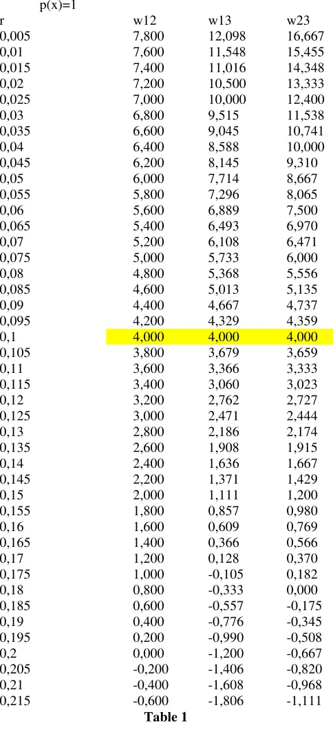
) 40 8 ( 12 r w r r w 10 3 ) 220 38 ( 13 r r w 10 1 ) 100 18 ( 23
p(x)=1
r w12 w13 w23
0,005 7,800 12,098 16,667
0,01 7,600 11,548 15,455
0,015 7,400 11,016 14,348
0,02 7,200 10,500 13,333
0,025 7,000 10,000 12,400
0,03 6,800 9,515 11,538
0,035 6,600 9,045 10,741
0,04 6,400 8,588 10,000
0,045 6,200 8,145 9,310
0,05 6,000 7,714 8,667
0,055 5,800 7,296 8,065
0,06 5,600 6,889 7,500
0,065 5,400 6,493 6,970
0,07 5,200 6,108 6,471
0,075 5,000 5,733 6,000
0,08 4,800 5,368 5,556
0,085 4,600 5,013 5,135
0,09 4,400 4,667 4,737
0,095 4,200 4,329 4,359
0,1 4,000 4,000 4,000
0,105 3,800 3,679 3,659
0,11 3,600 3,366 3,333
0,115 3,400 3,060 3,023
0,12 3,200 2,762 2,727
0,125 3,000 2,471 2,444
0,13 2,800 2,186 2,174
0,135 2,600 1,908 1,915
0,14 2,400 1,636 1,667
0,145 2,200 1,371 1,429
0,15 2,000 1,111 1,200
0,155 1,800 0,857 0,980
0,16 1,600 0,609 0,769
0,165 1,400 0,366 0,566
0,17 1,200 0,128 0,370
0,175 1,000 -0,105 0,182
0,18 0,800 -0,333 0,000
0,185 0,600 -0,557 -0,175
0,19 0,400 -0,776 -0,345
0,195 0,200 -0,990 -0,508
0,2 0,000 -1,200 -0,667
0,205 -0,200 -1,406 -0,820
0,21 -0,400 -1,608 -0,968
[image:5.482.138.380.74.606.2]0,215 -0,600 -1,806 -1,111
And also the w-r relation:
Figure 1.
About the capital intensity (in price terms) stand the following3: From the production prices system stands:
( )
q q
w
w K R r K
R r
Κq is the capital intensity in the typical subsystem q. Therefore the capital intensities Κij , i≠j, i,j=1,2,3 are:
12
8 40 0,2
r K
r
13
38 220 3 10
19 110
r r K
r
23
18 100 1 10
9 50
r r K
r
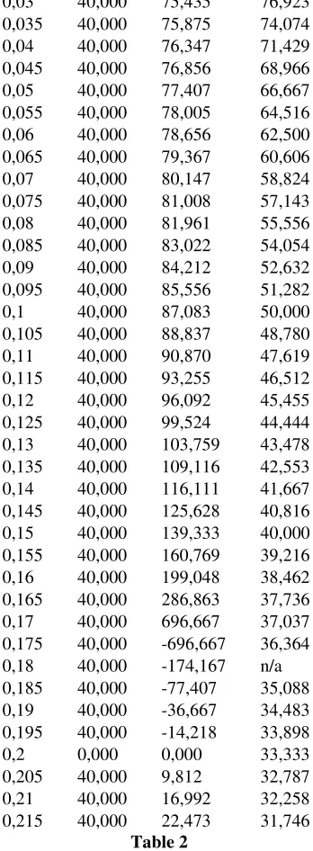
For the capital intensities the following results occur:
r k12 k13 k23
0,005 40,000 73,631 95,238
0,01 40,000 73,948 90,909
0,015 40,000 74,284 86,957
0,02 40,000 74,643 83,333
0,025 40,000 75,026 80,000
3 G.Stamatis (1997a)
w-r για P(x)=1
-5,000 0,000 5,000 10,000 15,000 20,000
0
,0
1
0
,0
3
0
,0
6
0
,0
8
0
,1
1
0
,1
3
0
,1
6
0
,1
8
0
,2
1
0
,2
3
0
,2
6
r
w
0,03 40,000 75,435 76,923
0,035 40,000 75,875 74,074
0,04 40,000 76,347 71,429
0,045 40,000 76,856 68,966
0,05 40,000 77,407 66,667
0,055 40,000 78,005 64,516
0,06 40,000 78,656 62,500
0,065 40,000 79,367 60,606
0,07 40,000 80,147 58,824
0,075 40,000 81,008 57,143
0,08 40,000 81,961 55,556
0,085 40,000 83,022 54,054
0,09 40,000 84,212 52,632
0,095 40,000 85,556 51,282
0,1 40,000 87,083 50,000
0,105 40,000 88,837 48,780
0,11 40,000 90,870 47,619
0,115 40,000 93,255 46,512
0,12 40,000 96,092 45,455
0,125 40,000 99,524 44,444
0,13 40,000 103,759 43,478
0,135 40,000 109,116 42,553
0,14 40,000 116,111 41,667
0,145 40,000 125,628 40,816
0,15 40,000 139,333 40,000
0,155 40,000 160,769 39,216
0,16 40,000 199,048 38,462
0,165 40,000 286,863 37,736
0,17 40,000 696,667 37,037
0,175 40,000 -696,667 36,364
0,18 40,000 -174,167 n/a
0,185 40,000 -77,407 35,088
0,19 40,000 -36,667 34,483
0,195 40,000 -14,218 33,898
0,2 0,000 0,000 33,333
0,205 40,000 9,812 32,787
0,21 40,000 16,992 32,258
[image:7.482.170.344.77.550.2]0,215 40,000 22,473 31,746
Figure 2
2,ij 1
p
For each technique’s w-r stands:
) 40 8 (
12 r
w
r r w
10 5
) 220 38 ( 13
23
(18 100 ) 3 10
r w
r
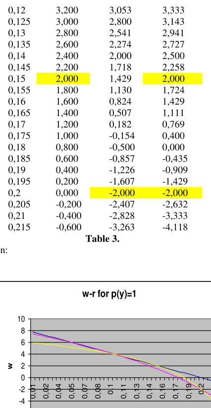
The results of the production prices for the first price normalization are: p(y)=1
r w12 w13 w23
0,005 7,800 7,455 5,932
0,01 7,600 7,306 5,862
0,015 7,400 7,155 5,789
0,02 7,200 7,000 5,714
0,025 7,000 6,842 5,636
0,03 6,800 6,681 5,556
0,035 6,600 6,516 5,472
0,04 6,400 6,348 5,385
0,045 6,200 6,176 5,294
0,05 6,000 6,000 5,200
0,055 5,800 5,820 5,102
0,06 5,600 5,636 5,000
0,065 5,400 5,448 4,894
0,07 5,200 5,256 4,783
0,075 5,000 5,059 4,667
0,08 4,800 4,857 4,545
0,085 4,600 4,651 4,419
0,09 4,400 4,439 4,286
0,095 4,200 4,222 4,146
0,1 4,000 4,000 4,000
0,105 3,800 3,772 3,846
0,11 3,600 3,538 3,684
0,12 3,200 3,053 3,333
0,125 3,000 2,800 3,143
0,13 2,800 2,541 2,941
0,135 2,600 2,274 2,727
0,14 2,400 2,000 2,500
0,145 2,200 1,718 2,258
0,15 2,000 1,429 2,000
0,155 1,800 1,130 1,724
0,16 1,600 0,824 1,429
0,165 1,400 0,507 1,111
0,17 1,200 0,182 0,769
0,175 1,000 -0,154 0,400
0,18 0,800 -0,500 0,000
0,185 0,600 -0,857 -0,435
0,19 0,400 -1,226 -0,909
0,195 0,200 -1,607 -1,429
0,2 0,000 -2,000 -2,000
0,205 -0,200 -2,407 -2,632
0,21 -0,400 -2,828 -3,333
[image:9.482.155.368.67.478.2]0,215 -0,600 -3,263 -4,118
Table 3. And w-r relation:
w-r for p(y)=1
-6 -4 -2 0 2 4 6 8 10
0
,0
1
0
,0
2
0
,0
4
0
,0
5
0
,0
7
0
,0
8
0
,1
0
,1
1
0
,1
3
0
,1
4
0
,1
6
0
,1
7
0
,1
9
0
,2
0
,2
2
r
w
Figure 3
Similar, based on the price system, occurs for the capital intensity:
( )
q q
w
w K R r K
R r
The capital intensities Κij ,i≠j, i,j=1,2,3 are the following:
12
8 40 0,2
r K
r
13
38 220 5 10
33 210
r r K
r
23
18 100 3 10
15 90
r r K
r
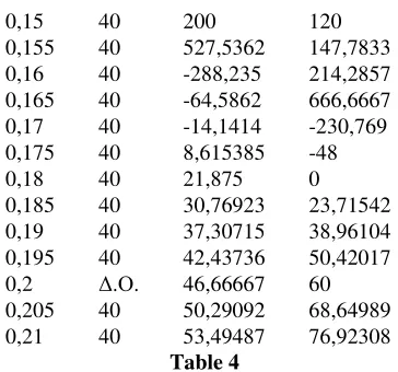
For the capital intensities the following hold:
r k12 k13 k32
0,005 40 48,99701 36,69404
0,01 40 49,65326 37,41746
0,015 40 50,33414 38,17235
0,02 40 51,04167 38,96104
0,025 40 51,77809 39,7861
0,03 40 52,54602 40,65041
0,035 40 53,34842 41,5572
0,04 40 54,18876 42,51012
0,045 40 55,07104 43,5133
0,05 40 56 44,57143
0,055 40 56,98122 45,68992
0,06 40 58,02139 46,875
0,065 40 59,12858 48,13394
0,07 40 60,31262 49,47526
0,075 40 61,58568 50,90909
0,08 40 62,96296 52,44755
0,085 40 64,4638 54,10536
0,09 40 66,11313 55,90062
0,095 40 67,94381 57,85593
0,1 40 70 60
0,105 40 72,34264 62,37006
0,11 40 75,05828 65,01548
0,115 40 78,27427 68,00349
0,12 40 82,18623 71,42857
0,125 40 87,11111 75,42857
0,13 40 93,59886 80,2139
0,135 40 102,6955 86,1244
0,14 40 116,6667 93,75
0,15 40 200 120
0,155 40 527,5362 147,7833
0,16 40 -288,235 214,2857
0,165 40 -64,5862 666,6667
0,17 40 -14,1414 -230,769
0,175 40 8,615385 -48
0,18 40 21,875 0
0,185 40 30,76923 23,71542
0,19 40 37,30715 38,96104
0,195 40 42,43736 50,42017
0,2 Δ.Ο. 46,66667 60
0,205 40 50,29092 68,64989
[image:11.482.165.347.68.238.2]0,21 40 53,49487 76,92308
Table 4
The above can be described in a figure:
Figure 4
It is obvious that in the case of price normalization with p(x)=1 there is only one switch point. In ccontroversy with price normalizing with p(Y)=1 there are tree switch points (it will be shown later if they are real or fake switch points) for r=0.05,r=0.1, r=0.15.
Normalized with p(x)=1, there is only one switch point4 in r=0.1. But things
change with price normalized with p(Y)=1. Once more the “real” switch point in r=0,1 and the “fake” switch points in r=0.05 and r=0.15 appear.
It has been shown that the switch point r=0.1 does not change with price normalization, in controversy with switch points r=0.05 ,r=0.15, which appear only when the normalization is p(Y)=1.
Based on w-r criterion, there is no significant reason, why the “fake” switch point, should not occur a transaction from a less profitable technique, to a more profitable5.
In other words for a given nominal wage, if r (which corresponds to the “fake” switch
4 A switch point can be found in the inner envelope, but it has not a significant economic meaning
5 By the so far analysis, it is evident that there is no relation between choosing a technique, according to the
[image:11.482.153.365.269.396.2]points) had not been chosen, then there would exist a technique that does not bring the maximum profit rate for the capitalists.
It is known from the bibliography6, that in special cases, is possible for the switch points (no matter if they are real or fake) to appear or disappear for a given price normalization even in the special case of the indecomposable single production techniques.
Bidard and Klimovsky, claim that the fake switch points can appear or disappear
only in special the case of joint production. From Bharadwaj’s paper7 is known that, it
is possible for two techniques to bring a different price vector in switch points, in the case the two techniques are not neighboring.
In this case not only the price vectors differ in switch points, but also the (dis)appearance of switch points, is affected by the changes in price normalization.
H.Kurz θαη N.Salvadori8
give a first definition, according to a technique is cost minimizing if there is no technique that brings extra profits9:
(1 )
(1 )
1
I I II II
I I I I
I
p r p A wl
p p A r wl
p d
In other words we import the prices that occur for RImax, in the profit maximization
criterion for technique [A lII, ]II . If term (3) is satisfied, no extra profits occur, and
technique [A lI, ]I is chosen as the cost minimizing one.
In the case of joint production the above terms will become:
(1 ) (1)
(1 ) (2)
1(3)
I II I II II
I I I I I I
I
p B r p A wl
p B p r p A wl
p d
, where r RImax For the following price normalizations:
1,ij 1
p
For each technique’s w-r stand:
) 40 8 (
12 r
w (4)
r r w
10 3
) 220 38 ( 13
(5)
r r w
10 1
) 100 18 (
23
(6)
First for technique (12) and for r Rmax(12) 0, 2the following will stand
The price vector for technique (12) is p12 [1,1].
Implying term (1) for techniques (13) and (23):
12 13 (1 ) 12 13 13(9)
p B r p A wl θαη
6 Th Mariolis, (1994)
7
Kr. Bharadway (1970)
8 H.D.Kurz and Neri Salvadori, (1995)
12 23 (1 ) 12 23 23(10)
p B r p A wl
12 23 (1 ) 12 23 23(10)
p B r p A wl
First we check term’s (9) direction in r=0.1:
48 70 48 70
In the same way we check the direction of term (10) in switch point r=0.1:
48 70 48 70
We conclude that in switch point r=0.1 production techniques (12) (13) and (23) are equivalent for prices of technique (12) and for technique p1=1.
2,ij 1
p
For each technique’s w-r:
) 40 8 (
12 r
w
r r w
10 5
) 220 38 ( 13
23
(18 100 ) 3 10
r w
r
First for technique (12) we have for r Rmax(12) 0, 2
12 [1,1]
p
10
Initially we check out what stands in switch point r=0.1. According to the cost minimization criterion:
12 13 12 13(1 ) 13 13 [40, 70] [48, 70]
p B p A r w
Therefore technique (13) minimizes cost as no extra profits occur from using this technique.
In the same way for technique (23):
12 23 12 23(1 ) 23 23 [48, 70] [48, 70]
p B p A r w
Technique (13) minimizes cost as no extra profits occur. In other words all the three techniques are cost minimizing.
It is evident that in “real” switch point r=0.1 all three techniques are equivalent. In the numerical example of Bidard and Klimovsky stands:
12 13 23 [1,1]
p p p
Furthermore we check what in “fake” switch point r=0.05 stands. According to the
cost minimization criterion:
12 13 12 13(1 ) 13 13 [40, 70] [48, 69]
p B p A r w
Therefore nothing can be said whether technique (23) minimizes cost or not. In other words the cost minimization criterion can not lead the system to cost minimizing technique.
In the same way for technique (23):
12 23 12 23(1 ) 23 23 [40, 70] [47.2, 68.2]
p B p A r w
Therefore nothing can be said whether technique (23) minimizes cost or not. In other words the cost minimization criterion can not lead the system to cost minimizing technique.
10
The price vectors for these techniques are:
12 13 23
[1,1] [0.778,1] [0.6,1]
p p p
In “fake” switch point r=0.15, also according to cost minimization criterion stand:
12 13 12 13(1 ) 13 13 [40, 70] [47.429, 70.428]
p B p A r w
Therefore technique (13) does not bring extra profits. In the same way for technique (23):
12 23 12 23(1 ) 23 23 [48, 70] [48, 71]
p B p A r w
Therefore technique (23) minimizes cost as occurs extra profits. In other words the cost minimizing technique is (23).
Last for the price vectors of the above techniques stand:
12 13 23
[1,1] [1.285,1] [1.667,1]
p p p
It is implied that in “fake switch” points, the intersected techniques have not the
same price vectors11. The last does not imply, nevertheless, that in fake switch points, no change in choice of techniques is occurred.
2.1. The General Case
In terms of the w-r criterion a non-decomposable productive12 joint production technique, let (a) is chosen instead of (b) when it stands:
a b
w w , that implies:
1 1
[ (1 )] [ (1 )]
a a a b b b
B A r y B A r y
, for normalization with y,y 013.
In the same way, in case we have more than two techniques:
a b c
w w w
1 1 1
[ (1 )] [ (1 )] [ (1 )]
a a a b b b c c c
B A r y B A r y B A r y
1
i
p y ,i=a,b,c.
First in the case of a switch point:
a b c
w w w
1 1 1
[ (1 )] [ (1 )] [ (1 )]
aBa Aa r y bBb Ab r y cBc Ac r y
In order for a switch point to be independent of price normalization it is necessary:
1 1 1
[ (1 )] [ (1 )] [ (1 )]
a a a b b b c c c
B A r B A r B A r
,
In other words, it is necessary all vectors 1
[ (1 )]
i i i
B A r
,for i=1,2,3 to be
equivalent14.
11 In this point, it is necessary to refer, that not only in the case of joint production but also in the case of non
neighboring single production techniques as well, the w-r criterion does not match with the cost minimization criterion.
12
In other words holds: [ (1 )]1 0
r A B
But in the case of fake switch points stands:
a b c
w w w
1 1 1
[ (1 )] [ (1 )] [ (1 )]
a a a b b b c c c
B A r y B A r y B A r y
Let the fake switch point –according to Bidard- to be found on the upper envelope of w-r curves, then:
a b c
w w w
1 1 1
[ (1 )] [ (1 )] [ (1 )]
a a a b b b c c c
B A r y B A r y B A r y
It is evident that in this case, according to the w-r criterion, the systems operates with either technique a or b. If the system operated with technique (c) then it operates
below it’s production potential15
.
Nevertheless the fake switch points, according to the w-r criterion are real switch points – although Bidard and Klimovsky claim the opposite. The fact that prices are
different in these points doesn’t seem to affect the final choice of techniques. The fact
that «fake switch points» appear and disappear16
, is a phenomenon that can be found, even in indecomposable single production systems17, and that because price normalizing affects the relative position of w-r curves18. But according to the cost minimization criterion we may decide which technique will be operated. The last is not something new, as it is know from bibliography19 that, in the case of joint production the w-r criterion and the cost minimization criterion do not come up to the same technological change decision.
3. Conclusions
In this analysis so far, an effort was made, to be shown in a numerical example of Bidard and Klimovsky, that the existence of “Fake” switch points does not change the aspect of choice of techniques.
The fact that in these switch point do not have the same price vectors, does not affect the choice of techniques. According not only to the w-r but to the cost minimization criterion as well, it is evident that a technique is chosen after all20.
An other characteristic, according to which the switch points called fake, was the fact that the switch points were appearing or disappearing with a change in price normalization. But in bibliography it is known that even the “real” switch points can appear or disappear with a change in price normalization
14 In the same way, in the case that two techniques i=a,b compete each other , the change of technique, in
only then unchanged, when the vectors can be compared 1
[ (1 )]
i i i
B A r
. In other words it is necessary
to be a order relation between them.
15
For the w-r relation: w K rn , where πε is the labor productivity and Κn the capital intensity in
price terms. In this case in order the relation wa wb wcto stand, the labor productivity should ceteris
paribus should be reduced (as for given r the capital intensity is constant). The last does not seem to be an orthological decision.
16The existence of real switch point in r=0.1, does not related with it’ s real switch point nature, but mostly
related of it’s property as the ratio of the compared typical subsystems
17 Th. Mariolis (1994)
18
This exalts choice of technique to a choice of typical subsystems instead.
19 G.Stamatis (1997)
The fact that in the above numerical example, the switch point in r=0.1 is not affected by a change in the standard commodity, is related with the fact that:
r=0.1 is the standard ration of surplus product to the used means of production/ used commodities.
In economic theory the ratio of surplus product to the used means of production/ used commodities is the same for all typical subsystems21.
In other words in mathematical terms, the rows and columns of the input matrices are linear dependent.
Consequently the case of Bidard’s and Klimovsky’s example is a special case, that
can not stand in general.
In the general case, the choice of technique depends on the price. The (re)switch points can appear or disappear with a change in the standard commodity.
Eventually when we refer to choice of techniques, we refer to choice of typical subsystems.
Finally not only the w-r criterion, but the cost minimization criterion as well, does not stand in general, because they are affected by the price normalization.
The only case that the choice of techniques is univocal is the charassofian systems of production and the corn economies. John von Neumann’s criterion22 can be counted as an application of the charassofian systems23.
4.References
Articles:
1. Christian Bidard and Edith Klimovsky (2004), Switches and fake switches in methods of production, Cambridge Journal of Economics 28:89-97
2. Bharadwaj, K., (1970). On the maximum number of switches between two
production systems. Schweizerische Zeitschrift für Volkswirtschaft und
Statistik 104, pp. 229–409
3. Bidard, C. (1990). An algorithmic theory of the choice of techniques, Econometrica, vol. 58, 839–85
4. Stamatis, Georg, Γηαηί ε ζύγθξηζε θαη θαηάηαμε ηερληθώλ είλαη αδύλαηε.
Τέπρε Πνιηηηθήο Οηθνλνκίαο, Ειιεληθά γξάκκαηα
5. Stamatis, Georg, (March/1999) Georg Charasoff: A Pioneer in the Theory of Linear Production Systems, Economic Systems Research, Volume: 11 , Issue: 1 , Pages: 15-30
6. Mariolis Th., (1994) Σρεηηθά κε ηε ζύγθξηζε ηερληθώλ παξαγωγήο ωο πξνο
ηελ θεξδνθνξία ηνπο, ηεύρε πνιηηηθήο Οηθνλνκίαο, ηεύρνο 14,
7. Stamatis G., (1996). Καηάμε ηερληθώλ θαη reswitching- Με αθνξκή έλα
άξζξν ηνπ Ch.Bidard, Τεύρε πνιηηηθήο νηθνλνκίαο, ηεύρνο 19,
21 Of course we refer to standard subsystems c.f. G.Stamatis (1999) and G. Stamatis, Γηαηίεζύγθξηζεθαη
θαηάηαμεηερληθώλείλαηαδύλαηε. ΤέπρεΠνιηηηθήοΟηθνλνκίαο, Ειιεληθάγξάκκαηα
22
G..Stamatis “John von Neumann’s Model of General Equilibrium” Indian Economic Journal, 1998; 45 (4)
8. Stamatis G., (Άλνημε 1997) Πεξί ηεο κνλνζήκαληεο θαηάηαμεο γξακκηθώλ
ηερληθώλ παξαγωγήο, ωο πξνο ηελ θεξδνθνξία ηνπο ή ηε θηήληα ηνπο, Τέπρε
πνιηηηθήο Οηθνλνκίαο, τεύχος 20, Εθδόζεηο Κξηηηθή.
9. Stamatis G., (1997),Η ζρέζε κεηαμύ ηνπ θξηηεξίνπ ηεο w-r ζρέζεο θαη ηνπ
θξηηεξίνπ ειαρηζηνπνίεζεο ηνπ θόζηνπο, Θέζεηο Νο 59,
10. Stamatis G., (1995) Πεξί ηεο νκαιήο ζπκπεξηθνξάο κε δηαζπώκελωλ
ζπζηεκάηωλ ζύλζεηεο παξαγωγήο, Τεύρε Πνιηηηθήο Οηθνλνκίαο, τεύχος 17.
11. Stamatis G., (1998) “John von Neumann’s Model of General Equilibrium” Indian Economic Journal 45
12. John von Neumann, (1935-36), A Model of General Economic Equilibrium", 1937, in K. Menger, editor, Ergebnisse eines mathematischen Kolloquiums (Translated and reprinted in RES, 1945)
Books:
1. Heinz D. Kurz and Neri Salvadori, (1995), Theory of production: A long-period analysis (Cambridge University Press, Cambridge)
2. Stamatis G. , (1995), Τν αδύλαηνλ κηαο ζύγθξηζεο ηερληθώλ ωο πξνο ηελ
θεξδνθνξία ηνπο θαη ηεο δηαπίζηωζεο κηαο επαλαρξεζηκνπνίεζεο ηερληθώλ, Πξνβιήκαηα ζεωξίαο γξακκηθώλ ζπζηεκάηωλ παξαγωγήο 1νο ηόκνο: Βαζηθά δεηήκαηα. Εθδόζεηο Κξηηηθή
3. Simpson D., (1975) General Equilibrium Analysis, An introduction Basil Blackwell, Oxford
4. Stamatis, Georg, Γηαηί ε ζύγθξηζε θαη θαηάηαμε ηερληθώλ είλαη αδύλαηε.
Τέπρε Πνιηηηθήο Οηθνλνκίαο, Ειιεληθά γξάκκαηα
5. Stamatis G., (1995), Γηα ην ηππηθό ππνζύζηεκα θαη ηε ζρέζε κεηαμύ
νλνκαζηηθνύ ωξνκηζζίνπ θαη πνζνζηνύ θέξδνπο- Μηα ζπκβνιή ζηε ζεωξία
ηωλ γξακκηθώλ ζπζηεκάηωλ παξαγωγήο, Πξνβιήκαηα ζεωξίαο γξακκηθώλ ζπζηεκάηωλ παξαγωγήο 1νο ηόκνο: Βαζηθά δεηήκαηα. Εθδόζεηο Κξηηηθή
6. Stamatis G., (1995), Η εμάξηεζε ηωλ ζρεηηθώλ ηηκώλ από ηελ ηππνπνίεζή
ηνπο, Μέξνο 1ν: Τππνπνίεζε θαη ζρεηηθέο ηηκέο ζε κε δηαζπώκελα
ζπζηήκαηα παξαγωγήο, Πξνβιήκαηα ζεωξίαο γξακκηθώλ ζπζηεκάηωλ παξαγωγήο 1νο ηόκνο: Βαζηθά δεηήκαηα. Εθδόζεηο Κξηηηθή
7. Stamatis G., Μηα γεληθή ιύζε ηνπ κνληέινπ γεληθήο ηζνξξνπίαο θαη