© 2016, IRJET ISO 9001:2008 Certified Journal Page 1620
Analytical Study of Algorithms for Mining Association Rules from
Probabilistic Databases and future possibilities
Niket Bhargava
1, Dr. Manoj Shukla
21
Department of Comp. Sc. & Engg., Mewar University, India
2Professor, Department of E&C, BCE, Mandideep, Bhopal, India
--- ---
Abstract — we consider the problem of discovering frequent item sets and association rules between items in a large database of transactional databases acquired under uncertainty. With each transaction associated is a probability gives the confidence that the transaction will occur. We discuss generalized algorithms for solving this problem that are fundamentally different from the known algorithms. Complete demonstration of algorithm presented and discussed in this paper. We also show how the best features of the algorithm can be combined into a business system.
Keywords: Data Mining, Big Data, Data Science,
Association Rule Mining, Probabilistic frequent patterns, probabilistic frequent rule.
1. INTRODUCTION
Now a days business databases not only recording exact transactions but at the same time also recording instable business circumstances into the data and hence with each and every possible transaction are associating a confidence or probability value that indicates strength by which the transaction will took place in real business world. Field of analytics specially predictive and prescriptive analytics playing critical role and are of great use to motivate probabilistic databases. Progress in digital bar-coding technology has made it possible for organizations to collect and store massive amounts of sales data, referred to as the basket data. A record in such data typically consists of the transaction date and the items bought in the transaction. Successful organizations view such databases as important pieces of the marketing infrastructure. They are interested in instituting information-driven marketing processes, managed by database technology, that enable marketers to develop and implement customized marketing programs and strategies [6].
The problem of mining association rules over market basket data was introduced in [4]. An example of such a rule might be that 98% of customers that purchase tires and auto accessories also get automotive services done. Finding all such rules is valuable for cross-marketing, cross-sell, up-sell, targeted marketing, product bundling and propensity focused attached mailing applications. Other applications
include catalog design, add-on sales, store layout, and customer segmentation based on buying patterns. The databases involved in these applications are very large. It is imperative, therefore, to have fast algorithms for this task[23].
The following is a formal statement of the problem [4]: Let I = { i1, i2, …, im} be a set of literals, called items. Let D be a set of transactions, where each transaction T is a set of items such that T ⊆ I. Associated with each transaction is a unique
identifier, called its TID. We say that a transaction T contains X, a set of some items in I, if X ⊆ T. An association rule is an implication of the form X ⇒ Y , where X ⊂ I, Y ⊂ I, and X∩Y = Ø. The rule X ⇒ Y holds in the transaction set D with
confidence c if c% of transactions in D that contain X also contain Y . The rule X⇒ Y has support s in the transaction set
D if s% of transactions in D contain X ∪ Y . Our rules are somewhat more general than in [4] in that we allow a consequent to have more than one item[23].Given a set of transactions D, the problem of mining association rules is to generate all association rules that have support and confidence greater than the user specified minimum support (called minsup) and minimum confidence (called minconf ) respectively. Our discussion is neutral with respect to the representation of Database D. For example, D could be a data file, a relational table, or the result of a relational expression[23].An algorithm for finding all association rules, henceforth referred to as the AIS algorithm, was presented in [4]. Another algorithm for this task, called the SETM algorithm, has been proposed in [13]. In this paper, we restudied algorithms, Apriori and Probabilistic_Apriori, that differ fundamentally from these algorithms.
© 2016, IRJET ISO 9001:2008 Certified Journal Page 1621 in [20]. If used for finding all association rules, this algorithm
will make as many passes over the data as the number of combinations of items in the antecedent, which is exponentially large. Related work in the database literature is the work on inferring functional dependencies from data [16]. Functional dependencies are rules requiring strict satisfaction. Consequently, having determined a dependency X → A, the algorithms in [16] consider any other dependency of the form X + Y → A redundant and do not generate it. The association rules we consider are probabilistic in nature. The presence of a rule X → A does not necessarily mean that X + Y → A also holds because the latter may not have minimum support. Similarly, the presence of rules X → Y and Y → Z does not necessarily mean that X → Z holds because the latter may not have minimum confidence. There has been work on quantifying the “usefulness” or “interestingness" of a rule [20]. What is useful or interesting is often application-dependent. The need for a human in the loop and providing tools to allow human guidance of the rule discovery process has been articulated, for example, in [7] [14].
Original Apriori works on exact non-probabilistic transactions. But transactions in real world occur with some uncertain probability. Data uncertainty is inherent in applications such as sensor monitoring systems, location-based services, and biological databases. To record and manage this vast amount of imprecise, uncertain information, probabilistic databases have been recently developed. In this paper, we study the discovery of frequent patterns and association rules from probabilistic databases under the Possible World Semantics. This is technically challenging, since a probabilistic database can have an exponential number of possible worlds. We evaluated probabilistic apriori algorithms, which discover frequent patterns in bottom-up manner likewise Apriori.
1.2 Problem Decomposition and Paper Organization
In case of non-probabilistic databases the problem of discovering all association rules can be decomposed into two subproblems[4]:
(1). Find all sets of items (itemsets) that have transaction support above minimum support. The support for an itemset is the number of transactions that contain the itemset. Itemsets with minimum support are called large itemsets, and all others small itemsets.
(2). Use the large itemsets to generate the desired rules. Here is a straightforward algorithm for this task. For every large itemset l, nd all non-empty subsets of l. For every such subset a, output a rule of the form a ⇒ (l - a) if the ratio of
support(l) to support(a) is at least minconf. We need to consider all subsets of l to generate rules with multiple consequents. Due to lack of space, we do not discuss this subproblem further, but refer the reader to [5] for a fast algorithm.
1.3 Discovering Large Itemsets
Algorithms for discovering large itemsets make multiple passes over the data. In the first pass, we count the support of individual items and determine which of them are large, i.e. have minimum support. In each subsequent pass, we start with a seed set of itemsets found to be large in the previous pass. We use this seed set for generating new potentially large itemsets, called candidate itemsets, and count the actual support for these candidate itemsets during the pass over the data. At the end of the pass, we determine which of the candidate itemsets are actually large, and they become the seed for the next pass. This process continues until no new large itemsets are found. The Apriori and AprioriTid algorithms differ fundamentally from the AIS[4] and SETM[13] algorithms in terms of which candidate itemsets are counted in a pass and in the way that those candidates are generated. In both the AIS and SETM algorithms, candidate itemsets are generated on-the-fly during the pass as data is being read. Specifically, after reading a transaction, it is determined which of the itemsets found large in the previous pass are present in the transaction. New candidate itemsets are generated by extending these large itemsets with other items in the transaction. However, the disadvantage with the Apriori and AprioriTID algorithms is that they generate the candidate itemsets to be counted in a pass by using only the itemsets found large in the previous pass. The basic intuition is that any subset of a large itemset must be large. Therefore, the candidate itemsets having k items can be generated by joining large itemsets having k-1 items, and deleting those that contain any subset that is not large. This procedure results in generation of a much smaller number of candidate itemsets. Apriori is explained in next section 2, than in section 3 problem of finding probabilistic frequent itemset is defined and in section 4 problem is solved fully on toy database.
2 APRIORI ALGORITHM
© 2016, IRJET ISO 9001:2008 Certified Journal Page 1622 pair, where TID is the identifier of the corresponding
transaction. We call the number of items in an itemset its size, and call an itemset of size k a k-itemset. Items within an itemset are kept in lexicographic order. We use the notation c[1].c[2]. . . c[k] to represent a k-itemset c consisting of items c[1], c[2], ... , c[k], where c[1] < c[2] < . . . < c[k]. if c is XY is an m-itemset, we also call Y an m-extension of X. Associated with each itemset is a count field to store the support for this itemset. The count field is initialized to zero when the itemset is first created. We summarize in table 1 the notation used in the algorithms.
TABLE -1: NOTATIONS FOR APRIORI
k -itemset An itemset having k items.
Lk Set of large k-itemsets Lk
#those with minimum support#. Each member of this set has two fields: i# itemset and ii# support count. Ck Set of candidate k-itemsets Ck
#potentially large itemsets#.
Each member of this set has two fields: i# itemset and ii# support count.
2.1 Algorithm Apriori
Figure 1 gives the Apriori algorithm. The first pass of the algorithm simply counts item occurrences to determine the large 1-itemsets. A subsequent pass, say pass k, consists of two phases. First, the large itemsets Lk-1 found in the (k-1)th pass are used to generate the
candidate itemsets Ck, using the apriori gen function
described in 2.1.1. Next the database is scanned and the support of candidates in Ck is counted. For fast
counting, we need to efficiently determine candidates in Ck that are contained in a given transaction t. See [5]
for a discussion of buffer management. 1) L1 = { large 1-itemsets } ;
2) for ( k = 2; Lk-1≠ Φ ; k++ ) do begin
3) Ck = apriori-gen(Lk-1 ); // New candidates
4) forall transactions t Є D do begin
5) Ct = subset(Ck , t); // Candidates contained in
t
6) forall candidates c Є Ct do 7) c.count++;
8) end
9) Lk = { c Є Ck | c.count ≥ minsup }
10) end
11) Answer = ∪k Lk ;
Figure -1: Algorithm Apriori 2.2 The apriori-gen function
The apriori-gen function takes as argument Lk-1, the set
of all large (k-1)-itemsets. It returns a superset of the set of all large k-itemsets. The function works as follows. 1 First, in the join step, we join Lk-1 with Lk-1 :
the logic implemented using sql query form is as follows;
(1) insert into Ck
select p.item[1], p.item[2], ... , p.item[k-1], q.item[k-1] from Lk-1 p, Lk-1 q
where p.item[1] = q.item[1], ... , p.item[k-2] = q.item[k-2], p.item[k-1] < q.item[k-1];
Next, in the prune step, we delete all itemsets c Є Ck
itemsets such that some (k-1)-subset of c is not in Lk-1
(1) forall itemsets c Є Ck do
forall (k-1)-subsets s of c do
if ( c not belongs to L[k-1] ) then delete c from Ck ;
3. Probabilistic FREQUENT PATTERN AND ASSOCIATION RULE MINING
In this section we will discuss mining uncertain database data with probabilistic certainty. Data uncertainty is inherent in many applications such as sensor monitoring systems, location-based services, and biological databases. To manage this vast amount of imprecise information, probabilistic databases have been recently developed. In this paper, we study the discovery of frequent patterns and association rules from probabilistic data under the Possible World Semantics. This is technically challenging, since a probabilistic database can have an exponential number of possible worlds. The data managed in many emerging applications is often uncertain. Integration and record linkage tools, for example, associate confidence values to the output tuples according to the quality of matching [34]. In structured information extractors, confidence values are appended to rules for extracting patterns from unstructured data [52]. In habitat monitoring systems, data collected from sensors like temperature and humidity are noisy [34]. The locations of users obtained through RFID and GPS systems are also imprecise [25, 39]. To handle these problems, probabilistic databases have been recently proposed, where uncertainty is treated as a “first-class citizen” [31, 34, 44, 33, 38]. Due to its simplicity in database design and query semantics, the tuple-uncertainty model is commonly used in probabilistic databases. Conceptually, each tuple carries an
existential probability attribute, which denotes the
© 2016, IRJET ISO 9001:2008 Certified Journal Page 1623
ID locatio
n time speed traffic weather . prob
t1 x
8-9pm 30-40 high Rain 0.1
t2 x
7-8am 80-90 low null 1.0
t3 x
8-9pm 80-90 low Foggy 0.5
t4 x
8-9pm 30-40 high Rain 0.2
t5 y
[image:4.595.42.262.101.198.2]2-3pm 50-60 low Sunny 1.0
Figure -2: A probabilistic database example
To interpret tuple uncertainty, the Possible World Semantics (or PWS in short) is often used [34]. Conceptually, a database is viewed as a set of deterministic instances (called possible worlds), each of which contains a set of zero or more tuples. A possible world for Figure 2 consists of the tuples { t2, t3, t5 }, existing with a probability of (1 - 0.1) x 1.0 x 0.5 x ( 1 - 0.2) x 1.0 = 0.036. Any query evaluation algorithm for probabilistic database has to be correct under PWS. That is, the results produced by the algorithm should be the same as if the query is evaluated on every possible world[34] Although PWS is intuitive and useful, evaluating queries under this notion is costly. This is because a probabilistic database has an exponential number of possible worlds. For example, the table in Figure 1 has 23 = 8 possible worlds. Performing query evaluation or data mining under PWS can thus be technically challenging. In fact, the mining of uncertain or probabilistic data has recently attracted research attention [26]. In [41], efficient clustering algorithms were developed to group uncertain objects that are close to each other. Recently, a Naive Bayes classifier has been developed [49]. The goals of this paper are: (1) propose a definition of frequent patterns and association rules for the tuple uncertainty model; and (2) develop efficient algorithm for mining frequent patterns and association rules.
Association rule Probability
r1: {location=x} ⇒ {time=8-9pm}
r2: {location=x} ⇒
{speed=80-90,traffic=low}
[image:4.595.40.297.526.590.2]0.15 0.49
Figure -3: Sample p-ARs derived from Figure 2 The frequent patterns discovered from probabilistic data are also probabilistic, to reflect the confidence placed on the mining results. Figure 3 shows two probabilistic frequent patterns (or p-FP) extracted from the database in Figure 2. A p-FP is a set of attribute values that occur frequently with
sufficiently high probabilities. The pmf of the number of tuples is the support count that contains a
pattern with specific probability. Under PWS, a database is a set of possible worlds, each of which records a (different) support of the same pattern. Hence, the support of a frequent pattern is a pmf. In figure 1, if we consider all possible worlds where { location = x }occurs three times, the pmf of { location
= x } with a support of 3 is 0.49. for the p-FP shown. Figure 3 displays their related probabilistic association rules (or p-ARs). Here, rule r2 suggests that with a 0.49 probability, 1) red-light violations occur frequently at location x and 2) when this happens, the involved vehicle is likely driving at a high speed amid low traffic. We will later explain more about the semantics of p-FP and p-AR. A simple way of finding p-FPs is to extract frequent pat- terns from every possible world. This is practically infeasible, since the number of possible worlds is exponentially large.
Prior work. [30] studied approximate frequent patterns on noisy data, while [42] examined
association rules on fuzzy sets. The notion of a “vague association rule” was developed in [43]. These solutions were not developed on probabilistic data models. For probabilistic databases, [32, 25] derived patterns based on their expected support counts. [54, 50] found that the use of expected support may render important patterns missing. They discussed the computation of the probability that a pattern is frequent. While [55] handled the mining of single items, our solution can discover patterns with more than one item. The data model used in [50] assumes that for each tuple, each attribute value has a
probability of being correct. This is different from the tuple-uncertainty model, which describes the joint probability of attribute values within a tuple. pmf evaluation method DC algorithm is asymptotically faster than the DP algorithms used in [54, 50], and is thus more scalable for large and dense datasets. To our best knowledge, none of the above works considered the important problem of generating association rules on probabilistic databases. This section is organized as follows. Section 3.1 introduces the notions of p-FPs and p-ARs. Sections 3.2 present our algorithms for mining p-FPs. Section 3.3 discusses fully solved example using dataset used in paper introduced Pascal algorithm. The CIPFP algorithm is described in section 5 and example is described in section 6
3.1 Problem Definition
We first review frequent patterns and association rules in Sections 3.1.1. Then, we discuss the
uncertain data model in Section 3.1.2. We present the problems of mining p-FPs and p-ARs, in Sections 3.1.3 and 3.1.4.
3.1.1 Frequent Patterns and Association Rules
A transaction is a set of items (e.g., goods bought by a customer in a supermarket). A set of items is also called an itemset or a pattern. Given a transaction database of size n and a pattern X, we use sup(X) to denote the support of X, i.e., the number of times that X appears in the database. A pattern X is frequent if:
© 2016, IRJET ISO 9001:2008 Certified Journal Page 1624 where minsup ∈ N ∩ [1, n] is the support threshold
[27].
Given patterns X and Y (with X∩Y = Ø), if pattern XY is frequent, then X is also frequent (called the
anti-monotonicity property). Also, X⇒Y is an association rule if
following conditions holds:
supp(XY) ≥ minsup (2) supp(XY)/supp(X) ≥ minconf (3)
sup(XY) / sup(X), denoted by conf(X⇒Y), is the confidence of X⇒Y, and minconf ∈ R ∩ (0, 1] is the confidence
threshold. To verify Equation 3, the values of sup(XY) and sup(X) have to be found first.
We remark that a transaction database is essentially a relational table with asymmetric binary attribute values. For example, the existence of item “apple” in a transaction is equivalent to a binary attribute of a tuple with a value of 1. This kind of attributes, assumed in this paper, is also considered by some mining algorithms (e.g., [27, 28]). To handle other attribute types (e.g., continuous and categorical), discretization and binarization techniques can be used to convert them to binary attributes [52].
3.2.2 The Possible World Semantics
We assume that each transaction has an existential probability, which specifies the chance that the transaction exists. Figure 4(a) illustrates this database, in which each transaction is a set of items represented by letters. This model has been used to capture uncertainty in many applications, including data streams[33] and geographical services[45]. Now, let P(E) be the probability that an event E occurs and PDB be probabilistic database of size n. Also, let Ti (where i = 1, ..., n ) be the ID of each tuple in PDB. Suppose Ti.S is the set of items contained in Ti, and Ti.p is the existential probability of Ti.
ID SetOfItems Probability/ confidence
T 1 {a, c, e, g, i} 0.6
T 2 {a, c, f, h} 0.5
T 3 {a, d, e, g, j} 0.7
T 4 {b, d, f, h, i} 1.0
Figure -4(a): A probabilistic database
Under PWS, PDB is a set of possible worlds W. Figure 4(b) lists all possible worlds for figure 4(a). Each Wi ε W exists with probability P(Wi). For example P(W2) = T1.p X ( 1 – T2.p) X ( 1 -T3.p) X T4.p or 0.09. The sum of possible world probabilities is one. Also, the number of possible worlds is exponentially large,
i.e. |w| = O( 2n). Our goal is to discover patterns and
rule using these possible worlds.
W Tuples in W Prob. W Tuples in W Prob.
W1 T4 0.06 W5 T1, T2, T4 0.09
W2 T1, T4 0.09 W6 T1, T3, T4 0.21
W3 T2, T4 0.06 W7 T2, T3, T4 0.14
W4 T3, T4 0.14 W8 T1, T2, T3, T4 0.21
Figure -4(b):Possible World for PDB in Figure 4(a)
3.2 Probabilistic Frequent Patterns
we first explain the concept of support for
probabilistic data. Given a pattern X, we denote its support in each world Wi as supi(X) is obtained by
counting the number of times X appears in Wi. Since each Wi exists with a probability, the support of X in PDB, i.e. sup(X), is a random variable. We denote fX(k) that the probability mass function (pmf) of
sup(X) can take. Specifically, fX(k) is the probability
that sup(X) = k, and fX(k) = 0 for any k ∉ [0,n]. We use
an array to store the non-zero values of fX, where
fX[k] = P(supp(X) = k). Figure 4(c) depicts the
support pmf of {a}. the probability that sup({a}) = 1 is 0.29.
DEFINITION 1. A pattern X is a probabilistic frequent pattern or p-FP in PDB if P(sup(X) ≥ minsup) ≥ minprob (4) where minprob є R ∩ (0,1] is the probability threshold.
Problem 1(p-FP Mining). Given PDB, minsup and minprob, return a set of {X, fX(k), where X is a p-FP
.As we will discuss, the pmfs obtained with p-FPs are essential to generating probabilistic association rules. There are methods to approximating and compressing pmfs (e.g., see [35]). Here we assume that the pmf is exact, but our solutions can be
extended to support these schemes. Next, we present a useful lemma.
Lemma 1 (Anti-monotonicity). If pattern X is a p-FP, then any pattern X' ⊂ X is also a p-FP.
The anti-monotonicity property is true for frequent patterns in exact data [27]. Lemma 1 allows us to stop examining a pattern, if any of its sub-pattern is not a p-FP. A FP X is said to be maximal if we cannot find another
[image:5.595.306.559.132.249.2] [image:5.595.35.266.531.678.2]© 2016, IRJET ISO 9001:2008 Certified Journal Page 1625 FP Y such that X ⊂ Y . A maximal p-FP can succinctly
represent a set of p-FPs when their supports are not concerned. Since the mining of maximal frequent patterns is an important problem [28] for exact data, we also study maximal p-FPs, together with free set, maximal set make a complete system, we study them too,:
Problem 2.1 (Free set p-FP Mining). Given a database PDB, minsup and minprob, return all minimal generators or free sets p-Fps.
Problem 2.2 (Maximal p-FP Mining). Given a database PDB, minsup and minprob, return all maximal p-Fps.
Problem 2.3 (closed p-FP Mining). Given a database PDB, minsup and minprob, return all closed p-FPs.
3.3 Probabilistic Association Rules
In a probabilistic database, the support counts of patterns are random variables. Let P (X⇒Y) be the probability that X⇒Y is an association rule. By Equations 2 and 3, we have: P (X⇒Y) =
P [sup(XY ) > minsup∧conf (X⇒Y) ≥ minconf] (5)
Definition 2. X⇒Y is a probabilistic association rule
(p-AR in short) if
P (X ⇒ Y ) ≥ minprob (6)
The problem of p-AR mining is defined as follows.
Problem 3 (p-AR Mining). Given minsup, minprob, minconf, and the p-FPs and their support pmfs obtained from Problem 1, derive all p-ARs and their probabilities.
A simple way of solving Problems 1, 2, and 3 is to expand PDB into all possible worlds, compute patterns and rules from each world, and then combine the results. If minsup=2, minconf=0.5, and minprob=0.2, for Figure 4(a), {a}⇒{c} is an association rule only in worlds W5 and W8 (Figure 4(c)), with P ({a}⇒{c}= Pr(W5) + Pr(W 8) = 0.09 + 0.21 = 0.3. Since
this is larger than 0.2, {a}⇒{c} is a p-AR. This method is not practical , due to the large number of possible worlds. To tackle Problems 1 and 2, proposed algorithms, namely probabilistic Apriori discussed and solved fully in next section 4.
4. Probabilistic Apriori using PWS fully Solved case
In this section we display the probabilistic Apriori using PWS fully Solved using toy database used in research paper by Bastides et. al. described algorithm Pascal. To solve Problem 1, we discussed the probabilistic-Apriori algorithm, which is an adaptation of the Apriori algorithm [27] for probabilistic databases. Specifically, probabilistic-Apriori uses the bottom-up framework [27]: using PWS.
4.1 Our Probabilistic Algorithm: Probabilistic Apriori
1. PDB Database making, 2. PWS making using PDB,
3. Define candidate C1 1-itemset equal to Item
Collection I.
4. PDB database scan for all c belongs to C1 to calculate support c.support. Store them in a list call it FP.
5. PWS database scan for all c in FP and all c.support where support is equal to “0” to “c.support” to evaluate fc[k] probability pmf support.
6. Determining Probabilistic Frequent Patterns using minsup and minprob. First compare minsup with c.support. If c.support ≥ minsup than using pmf for pattern c in C1 compare fc[k] ≥ minprob. Collect all c in PFP and assign it to L1 all along with valid frequent
probable support and probability. Call it L1.
7.1) L1 = { large 1-itemsets } ;
7.2) for ( k = 2; Lk-1≠ Φ ; k++ ) do begin
7.3) Ck=apriori-gen(Lk-1 ); // New candidates
7.4) forall transactions t Є PDB do begin
7.5) Ct=subset(Ck,t);//Candidates contained in t
7.6) forall candidates c Є Ct do 7.7) c.count++;
7.8) end
7.9) FP = { c Є Ck | c.count ≥ minsup }
7.10) forall fp Є FP
7.11) from k = 0 to fp.support
7.12) W = w Є PWS exactly with size k times k number of transactions
7.13) Ffp[k].prob++; 7.14) end
7.15) PFP = { FP Є FPk | Ffp[k].prob ≥ minprob }
7.15) Lk = PFP
7.16) end
7.17) Answer = ∪k Lk ;
Figure -5: Probabilistic Apriori Algorithm
A. The apriori-gen function
The apriori-gen function takes as argument Lk-1, the set of
all large (k-1)-itemsets. It returns a superset of the set of all large k-itemsets. The function works as follows. 1 First, in the join step, we join Lk-1 with Lk-1 : the logic is in the
form of sql query form is as follows; (1) insert into Ck
select p.item[1], p.item[2], ... , p.item[k-1], q.item[k-1]
from Lk-1 p, Lk-1 q
where p.item[1] = q.item[1], ... , p.item[k-2] = q.item[k-2], p.item[k-1] < q.item[k-1];
Next, in the prune step, we delete all itemsets c Є Ck
itemsets such that some (k-1)-subset of c is not in Lk-1.
© 2016, IRJET ISO 9001:2008 Certified Journal Page 1626 forall (k-1)-subsets s of c do
if ( c not belongs to Lk-1 ) then
delete c from Ck ;
4.2 Solved Example Probabilistic Apriori
[image:7.595.305.567.84.307.2]This section discusses the solved example of probabilistic Apriori on toy database. To explain fully general version is solved to full length. The database used is same as used is paper which presented Pascal Algorithm extended to include the transaction level existential probability and time stamp for time at which transaction took place. Figure 6 depicts Pascal Transaction Temporal Dataset with Probabilistic Confidence. For our Probabilistic Apriori algorithm only column TID, SetOfItems, and Probabilistic/Confidence are of importance or relevant.
TID SetOfItems TimeStamp Key ty/ConfidenProbabili ce
T1 A, B, C, F 1 ? 0.6 T2 B, C, E, F 2 ? 0.5 T3 A, B, C, E, F 3 ? 0.7
T4 B, E, F 4 ? 0.4
[image:7.595.35.293.297.415.2]T5 A, B, C, E, F 5 ? 1.0
Figure -6: PDB for Pascal Transactional Temporal Dataset with Probabilistic Confidence
Using concepts of Possible World Semantics in earlier sections, on database presented in Figure 6 we calculated PWS, which is available in Figure 7.
Wor lds
Transact ionInWo
rld
WorldProbalityCalcul
ation WorldProbablity
W1 T5 (1-0.6)*(1-0.5)*(1-0.7)*(1-0.4)*(1.0) 0.036
W2 T1T5 ( 0.6 )*(1-0.5)*(1-0.7)*(1-0.4)*(1.0) 0.054
W3 T2T5 (1-0.6)*( 0.5 )*(1-0.7)*(1-0.4)*(1.0) 0.036
W4 T3T5 (1-0.6)*(1-0.5)*( 0.7 )*(1-0.4)*(1.0) 0.084
W5 T4T5 (1-0.6)*(1-0.5)*(1-0.7)*( 0.4 )*(1.0) 0.024
W6 T1T2T5 ( 0.6 )*( 0.5 )*(1-0.7)*(1-0.4)*(1.0) 0.054
W7 T1T3T5 ( 0.6 )*(1-0.5)*( 0.7 )*(1-0.4)*(1.0) 0.126
W8 T1T4T5 ( 0.6 )*(1-0.5)*(1-0.7)*( 0.4 )*(1.0) 0.036
W9 T2T3T5 (1-0.6)*( 0.5)*( 0.7)*(1-0.4)*(1.0) 0.084
W10 T2T4T5 (1-0.6)*( 0.5 )*(1-0.7)*( 0.4 )*(1.0) 0.024
W11 T3T4T5 (1-0.6)*(1-0.5)*( 0.7 )*( 0.4 )*(1.0) 0.056
W12 T1T2T3T5 ( 0.6 )*( 0.5 )*( 0.7 )*(1-0.4)*(1.0) 0.126
W13 T1T2T4T5 ( 0.6 )*( 0.5 )*(1-0.7)*( 0.4 )*(1.0) 0.036
W14 T1T3T4T5 ( 0.6 )*( 1- 0.5 )*( 0.7 )*( 0.4 )*(1.0) 0.084
W15 T2T3T4T5 ( 1-0.6 )*( 0.5 )*( 0.7 )*( 0.4 )*(1.0) 0.056
W16 TIT2T3T4T5 ( 0.6 )*( 0.5 )*( 0.7 )*( 0.4 )*(1.0) 0.084
Figure -7: PWS for PDB for Pascal Transactional Temporal Dataset with Probabilistic Confidence The collection of Items for figure 6 PDB contains 6 individual items, let say I is the set of these items. Hence I = { A, B, C, D, E, F }, For this example minsup is 2/5 that is 40%. As total number of transactions in database i.e. the size of database n is 5. So, the threshold for minsup will be given by (5 * 40 ) /100, i.e 2. So, minsup is 2, let minprob is 0. We are taking minprob 0 to show that algorithm will behave exactly as apriori behave when no probabilistic transaction is considered. This is equivalent to treating all transactions having certainty or probability of 1 to occur. All the elements which belongs to collection I will become the candidate pattern, as the individual items themselves are used as patterns we call them 1-itemset. The collection of candidate 1-itemset denoted as C1 is as follows: C1 = {
{A}, {B},{C},{D},{E},{F}} for each element c belongs to C1
we calculate its support in database PDB Figure 6. For all itemset the PDB database scan output is as follows:
Pattern/1-itemset Support in PDB
{A} 3
{B} 4
{C} 4
{D} 1
{E} 4
{F} 5
Figure -8: C1 and its Support Count
In the figure 8 if we compare support of respective patterns we found that pattern {D} has a support 1 which is less than the minimum support. sup({D}) < minsup. So the set of frequent 1-itemset FP1 will contain all 1-itemset
from figure 8 but not {D}.This set of frequent 1-itemset FP1 is as follows;
[image:7.595.32.554.411.774.2]© 2016, IRJET ISO 9001:2008 Certified Journal Page 1627
itemset
{A} 3
{B} 4
{C} 4
{E} 4
{F} 5
Figure -9: FP1 set of frequent 1-itemset
Now we use patterns in FP1 one by one to calculate their
existential probability. For this we first scan PDB and extract the TIDs in which pattern is present. For
combination of length equal to in range for support from 0 to c.support we start scan of PWS rows and sum up the provabilities of Wi in which exactly the number of
transaction present, here the number of transaction which occurred in Wi is determined for every support from 0 to c.support. For example we want to determine existential probability of frequent 1-itemset {A} to determine probabilistic frequent pattern {A} is or not. First, we scan PDB and found that T1, T3, T5 contains {A}. {A}.support is 3. So for transaction combination length of 0, 1, 2, and 3, are possible k th support for {A} in PDB. Let say for example support 1 of pattern {A}, exactly for the count of 1, number of transactions that have {A}, Wi will form universe, means any Wi that contain exactly one time any of the {A}.Ti, i.e., Wi exactly contain either one of T1, or T2, or T2 but not T1T2, T1T3 or T2T3 or T1T2T3 together, all their probabilities will be summed up. For {A}.support is 1, PWS is W1W3W5W10 with probability 0.036, 0.036, 0.024, 0.024 summed up to 0.12, this 0.12 is existential probability of pattern {A} when its support is 1. Like wise we calculate for all fp belongs to FP1. The following figure
10 summaries C1 PFP1 patterns with their support pmf
values. “-” represents not required status.
Support\Pat
tern {A} {B} {C} {D} {E} {F}
0 0 0 0 0.4 0 0
1 0.12 0.09 0.06 0.6 0.09 0.036
2 0.46 0.36 0.29 - 0.36 0.198
3 0.42 0.41 0.44 - 0.41 0.380
4 - 0.14 0.21 - 0.14 0.246
5 - - - 0.140
Figure -10: C1 candidate PFP1 patterns with their support
pmf values
If we compare all 1-itemset support pmf values against minprob we will get PFP 1-itemset. For minprob “0” we will have entire Figure 10 as probabilistic frequent PFP1.
So, now using all patterns in PFP1 we will continue and
assign this collection to L1 and call apriori_gen on all
probabilistically frequent 1-itemset patterns in L1 to
generate candidate 2-itemset C2. Using PDB database scan
we count their support.
Pattern/2-itemset PDB Support in
{AB} 2
{AC} 3
{AE} 2
{AF} 3
{BC} 3
{BE} 4
{BF} 4
{CE} 3
{CF} 4
[image:8.595.310.502.148.348.2]{EF} 4
Figure -11: C2 and its Support Count
All pattern in Figure 11 are frequent. So, frequent 2-itemset will be as following in figure 12.
Pattern/2-itemset PDB Support in
{AB} 2
{AC} 3
{AE} 2
{AF} 3
{BC} 3
{BE} 4
{BF} 4
{CE} 3
{CF} 4
{EF} 4
Figure -12: FP2 and its Support Count
The candidate for PFP will be as following in figure 13.
Patte rn> Supp ortV
{A
B} {AC} {AE} {AF} {BC} {BE} {BF} {CE} {CF} {EF}
0 0 0 0 0 0 0 0 0 0 0 1 0.3 0.1
2 0.3 0.12 0.15 0.09 0.09 0.15 0.06 0.09 2 0.7 0.4
[image:8.595.308.504.383.589.2]© 2016, IRJET ISO 9001:2008 Certified Journal Page 1628 2 2 5 1 1 5 4 1
4 - - - 0.1
4 0.14 - 0.21 0.14 5 - - - -
Figure -13: C2 candidate PFP2 patterns with their support
pmf values.
All candidate PFP2 are probabilistic frequent hence we treat
patterns in figure 13 as PFP and finally as L2. These 2-itemset
probabilistically frequent patterns in L2 will be used to
generate candidate 3-itemset patterns.
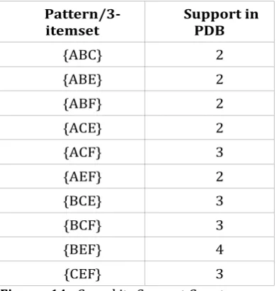
Pattern/3-itemset Support in PDB
{ABC} 2
{ABE} 2
{ABF} 2
{ACE} 2
{ACF} 3
{AEF} 2
{BCE} 3
{BCF} 3
{BEF} 4
[image:9.595.305.557.61.291.2]{CEF} 3
Figure -14.: C3 and its Support Count
All pattern in Figure 14 are frequent. So, frequent 3-itemset will be as following in figure 15.
Pattern/3-itemset Support in PDB
{ABC} 2
{ABE} 2
{ABF} 2
{ACE} 2
{ACF} 3
{AEF} 2
{BCE} 3
{BCF} 3
{BEF} 4
[image:9.595.36.233.236.442.2]{CEF} 3
Figure -15: FP3 and its Support Count
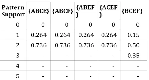
The candidate for PFP will be as following in figure 16.
Patt {A {AB {A {AC {AC {A {BC {B {B {CEF
ern Supp ort
BC
} E} BF} E} F} EF} E} CF} EF} }
0 0 0 0 0 0 0 0 0 0 0 1 0.2
64 0.264 0.264 0.264 0.264 0.264 0.15 0.15 0.09 0.15 2 0.7
36 0.736 0.736 0.736 0.736 0.736 0.50 0.50 0.36 0.50 3 - - - 0.3
5 0.35 0.41 0.35 4 - - - 0.1
4 - 5 - - - -
Figure -16: C3 candidate PFP3 patterns with their support
pmf values.
All candidate PFP3 are probabilistic frequent hence we
treat patterns in figure 16 as PFP and finally as L3. These
3-itemset probabilistically frequent patterns in L3 will be
used to generate candidate 4-itemset patterns, which are as follows;
Pattern/4-itemset Support in PDB
{ABCE} 2
{ABCF} 2
{ABEF} 2
{ACEF} 2
[image:9.595.308.507.394.516.2]{BCEF} 3
Figure -17: C4 and its Support Count
All pattern in Figure 17 are frequent. So, frequent 3-itemset will be as following in figure 18.
Pattern/4-itemset Support in PDB
{ABCE} 2
{ABCF} 2
{ABEF} 2
{ACEF} 2
[image:9.595.35.231.475.678.2]{BCEF} 3
Figure -18: FP4 and its Support Count
[image:9.595.307.505.548.662.2]© 2016, IRJET ISO 9001:2008 Certified Journal Page 1629
Pattern
Support {ABCE} {ABCF} {ABEF} {ACEF} {BCEF}
0 0 0 0 0 0
1 0.264 0.264 0.264 0.264 0.15 2 0.736 0.736 0.736 0.736 0.50
3 - - - - 0.35
4 - - - -
-5 - - - -
-Figure -19: C4 candidate PFP4 patterns with their support
pmf values.
All candidate PFP4 are probabilistic frequent hence we
treat patterns in figure 19 as PFP and finally as L4. These
4-itemset probabilistically frequent patterns in L4 will be
used to generate candidate 5-itemset patterns, which are as follows;
Pattern/4-itemset Support in PDB
{ABCE} 2
Figure -20: C5 and its Support Count
All pattern in Figure 20 are frequent. So, frequent 3-itemset will be as following in figure 21.
Pattern/5-itemset Support in PDB
{ABCEF} 2
Figure -21: P5 and its Support Count
The candidate for PFP will be as following in figure 22.
Support\Pattern {ABCEF}
0 0
1 0.264
2 0.736
3 -
4 -
[image:10.595.36.286.96.230.2]5 -
Figure -22: C5 candidate PFP5 patterns with their support
pmf values.
All candidate PFP5 are probabilistic frequent hence we
treat patterns in figure 22 as PFP and finally as L5. These
5-itemset probabilistically frequent patterns in L5 will be
used to generate candidate 6-itemset patterns. But no
more new candidate 6-itemset are possible so algorithm execution stops here.
5. CONCLUSION
Real world application requires mining of patterns occurrences of which are random or uncertain in nature. This uncertain is introduced in the system because of many parameters which may be endogenous or exogenous. This uncertainty is introduced many time because of uncertainty in competency of operator involved in transactional process. Uncertainty may be introduced due to limitation of measurement machines, instruments, and/or procedure. So, to encompass this truth of process we studied and suggested a mining procedure that can be used to answer queries which or otherwise only possible to answer on certain data using data mining techniques. To best of our knowledge the steps we carried out are not discuss to this much extent in any paper. Algorithm finally converged. 32 probabilistic frequent patterns were generated when we took the probability of transactions equal to one, i.e. minimum threshold is considered as 0. Many variations in implementation of the algorithm are possible. Also how to select suitable minprob threshold is, depending on this algorithm can be modified. In future we will implement the algorithm with possible alternate implementation as well as mechanism to support selection of minimum support threshold, and selection of minimum probability threshold.
REFERENCES
[1] R. Agrawal, C. Faloutsos, and A. Swami. Effcient similarity search in sequence databases. In Proc. of the Fourth International Conference on Foundations of Data Organization and Algorithms, Chicago, October 1993.
[2] R. Agrawal, S. Ghosh, T. Imielinski, B. Iyer, and A. Swami. An interval classi er for database mining applications. In Proc. of the VLDB Conference, pages 560{573, Vancouver , British Columbia, Canada, 1992. [3] R. Agrawal, T. Imielinski, and A. Swami. Database mining: A performance perspective. IEEE Transactions on Knowledge and Data En- gineering, 5(6):914{925, December 1993. Special Issue on Learning and Discovery in Knowledge- Based Databases. [4] R. Agrawal, T. Imielinski, and A. Swami. Mining association rules between sets of items in large databases. In Proc. of the ACM SIGMOD Con- ference on Management of Data, Washington, D.C., May 1993. [5] R. Agrawal and R. Srikant. Fast algorithms for mining association rules in large databases. Re- search Report RJ 9839, IBM Almaden Research Center, San Jose, California, June 1994.
[6] D. S. Associates. The new direct marketing. Business One Irwin, Illinois, 1990.
[image:10.595.35.238.511.675.2]© 2016, IRJET ISO 9001:2008 Certified Journal Page 1630 [8] L. Breiman, J. H. Friedman, R. A. Olshen, and C. J.
Stone. Classi cation and Regression Trees. Wadsworth, Belmont, [9] P. Cheeseman et al. Autoclass: A bayesian classi cation system. In 5th Int'l Conf. on Machine Learning. Morgan Kaufman, June 1988.
[10] D. H. Fisher. Knowledge acquisition via incre-mental conceptual clustering. Machine Learning, 2(2), 1987.
11] J. Han, Y. Cai, and N. Cercone. Knowledge discovery in databases: An attribute oriented approach. In Proc. of the VLDB Conference, pages 547{559, Vancouver, British Columbia, Canada, 1992. [12] M. Holsheimer and A. Siebes. Data mining: The search for knowledge in databases. Technical Report CS-R9406, CWI, Netherlands, 1994.
[13] M. Houtsma and A. Swami. Set-oriented mining of association rules. Research Report RJ 9567, IBM Almaden Research Center, San Jose, Cali- fornia, October 1993. [14] R. Krishnamurthy and T. Imielinski. Practi- tioner problems in need of database research: Re- search directions in knowledge discovery. SIG- MOD RECORD, 20(3):76{78, September 1991.
[15] P. Langley, H. Simon, G. Bradshaw, andJ. Zytkow. Scienti c Discovery: Computational Explorations of the Creative Process. MIT Press, 1987.
[16] H. Mannila and K.-J. Raiha. Dependency inference. In Proc. of the VLDB Conference, pages 155{158, Brighton, England, 1987.
[17] H. Mannila, H. Toivonen, and A. I. Verkamo. E cient algorithms for discovering association rules. In KDD-94: AAAI Workshop on Knowl- edge Discovery in Databases, July 1994.
[18] S. Muggleton and C. Feng. E cient induction of logic programs. In S. Muggleton, editor, Inductive Logic Programming. Academic Press, 1992.
[19] J. Pearl. Probabilistic reasoning in intelligent systems: Networks o plausible inference, 1992.
[20] G.Piatestsky-Shapiro. Discovery, analy- sis, and presentation of strong rules. In G. Piatestsky-Shapiro, editor, Knowledge Dis- covery in Databases. AAAI/MIT Press, 1991.
[21] G. Piatestsky-Shapiro, editor. Knowledge Dis- covery in Databases. AAAI/MIT Press, 1991.
[22] J. R. Quinlan. C4.5: Programs for Machine Learning. Morgan Kaufman, 1993.
[23] Rakesh Agrawal, Ramakrishnan Srikant: “Fast Algorithms for Mining Association Rules” Proceedings of the 20th VLDB Conference Santiago, Chile, 1994
[24]Liwen Sun, Reynold Cheng, David W. Cheung, Jiefeng Cheng, “Mining Uncertain Data with Probabilistic
Guarantees”, KDD’10, July 25–28, 2010, Washington, DC, USA. Copyright 2010 ACM 978-1-4503-0055-1/10/07 [25] A. Deshpande et al. Model-driven data acquisition in sensor networks. In VLDB, 2004.
[26] C. Aggarwal, Y. Li, J. Wang, and J. Wang. Frequent pattern mining with uncertain data. In KDD, 2009. [27] C. Aggarwal and P. Yu. A survey of uncertain data algorithms and applications. IEEE Transactions on Knowledge and Data Engineering, 21(5), 2009.
[28] R. Agrawal and R. Srikant. Fast algorithms for mining association rules in large databases. Technical report, RJ 9839, IBM, 1994.
[29] R. Bayardo, Jr. Efficiently mining long patterns from databases. In SIGMOD, 1998.
[30] D. Burdick, M. Calimlim, J. Flannick, J. Gehrke, and T. Yiu. MAFIA: A maximal frequent itemset algorithm. IEEE Transactions on Knowledge and Data Engineering, 17, 2005.
[31] H. Cheng, P. Yu, and J. Han. Approximate frequent itemset mining in the presence of random noise. Soft Computing for Knowledge Discovery and Data Mining, 2008.
[32] R. Cheng, D. Kalashnikov, and S. Prabhakar.
Evaluating probabilistic queries over imprecise data. In SIGMOD, 2003.
[33] C. K. Chui, B. Kao, and E. Hung. Mining frequent itemsets from uncertain data. In PAKDD, 2007. [34] G. Cormode and M. Garofalakis. Sketching probabilistic data streams. In SIGMOD, 2007.
[34] N. Dalvi and D. Suciu. Efficient query evaluation on probabilistic databases. In VLDB, 2004.
[35] M. Garofalakis and A. Kumar. Wavelet synopses for general error metrics. ACM Transactions on Database Systems, 30(4), 2005.
[36] K. Gouda and M. J. Zaki. GenMax: An efficient algorithm for mining maximal frequent itemsets. Data Mining and Knowledge Discovery, 11(3), 2005.
[37] R. Hogg, A. Craig, and J. Mckean. Introduction to Mathematical Statistics (6th ed.). Prentice Hall, 2004. [38] J. Huang et al. MayBMS: A Probabilistic Database Management System. In SIGMOD, 2009.
[39] N. Khoussainova, M. Balazinska, and D. Suciu.Towards correcting input data errors probabilistically using integrity constraints. In MobiDE, 2006.
[40] D. Knuth. The art of computer programming, vol. 3.Addison Wesley, 1998.
[41] H. Kriegel and M. Pfeifle. Density-based clustering of uncertain data. In KDD, 2005.
© 2016, IRJET ISO 9001:2008 Certified Journal Page 1631 [44] M. Mutsuzaki et al. Trio-one: Layering uncertainty and
lineage on a conventional dbms. In CIDR, 2007.
[45] M. Yiu et al. Efficient evaluation of probabilistic advanced spatial queries on existentially uncertain data. IEEE Transactions on Knowledge and Data Engineering, 21(9), 2009.
[46]R. Motwani and P. Raghavan. Randomized algorithms.Cambridge University Press, New York, NY, USA, 1995.
[47] A. Oppenheim, R. Schafer, and J. Buck. Discrete-time signal processing (2nd ed.). Prentice Hall, 1999.
[48] P. Sistla et al. Querying the uncertain position of moving objects. In Temporal Databases: Research and Practice. Springer Verlag, 1998.
[49] J. Ren, S. Lee, X. Chen, B. Kao, R. Cheng, and D. Cheung. Na¨ıve Bayes Classification of Uncertain Data. In ICDM, 2009.
[50] T. Bernecker et al. Probabilistic frequent itemset mining in uncertain databases. In KDD, 2009.
[51] T. Jayram et al. Avatar information extraction system. IEEE Data Engineering Bulletin, 29(1), 2006. [52] P. Tan, M. Steinbach, and V. Kumar. Introduction to Data Mining. Pearson Education, 2006.
[53] C. Yang and W. Najm. Examining driver behavior using data gathered from red light photo enforcement cameras. Journal of Safety Research, 38(3), 2007. [54] Q. Zhang, F. Li, and K. Yi. Finding frequent items in probabilistic data. In SIGMOD, 2008.
BIOGRAPHIES
Niket Bhargava, born in state is MP in the India, on July 6, 1978. He graduated from the Oriental Institute of Science And Technology, Bhopal, and after qualifying in GATE, completed his Master in Technology from the RGTU- the technical university of MP, India. His employment experience included the 10 years as Teacher in Top Most Ranking Institutions of state of MP,and Industry experience of BI product development. Presently, he is pursuing his PhD in CSE with focus on business applications of data mining , data
science, big data techniques for Business Intelligence. Dr. MANOJ SHUKLA, is working as professor in BCE,