ISSN: 1992-8645 www.jatit.org E-ISSN: 1817-3195
2497
ENHANCING VISUAL PROPERTIES OF GRAPH
COMMUNITIES
JAMAL ALSAKRAN
The University of Jordan, Computer Science Department, Jordan
E-mail: [email protected]
ABSTRACT
Systems that take the form of graphs of nodes and edges are common in various fields of study such as biology, and social and organizational studies. Typically, these systems exhibit community structure that corresponds to modular decomposition of functionality and common features of interest. In this paper, we endeavor to contribute to the efforts to enhance the visual representation of community structure. We propose refinements to the visual layout produced by force-layout model and treemap to foster desirable visual properties. Experiments are conducted on real world datasets to show the effectiveness of our approach and discuss its impact on the system overall performance.
Keywords: Graph Community, Modularity, Visualization, Treemap, Force-layout
1. INTRODUCTION
In a graph of nodes and edges, finding communities (or clusters) consists of partitioning the graph into clusters such that there are many edges within clusters and relatively few edges between clusters. The need for discovering communities has emerged from the fact that most systems that take the form of graph exhibit community structure and finding those communities can reveal valuable information. For example, communities in collaboration network reveal research groups and highlight the pattern of collaboration between research fields [1]. Uncovering the underlying modules of a complex metabolic network shows that cellular functionality can be seamlessly partitioned into a collection of modules each of which performs an identifiable task, separable from the functions of other modules [2] [3]. In social networks, community structure corresponds to relationships between individuals arising due to personal, political and cultural reasons, giving rise to informal communities. Understanding informal communities underlying the formal organization is a key element in a successful management [4].
Community detection has received a great attention and a wide range of approaches has been presented in the literature [5] [6]. The various approaches employ measures, e.g. modularity [6] to ensure the results agree with some desirable properties, for example, high edge density of
clusters and cluster separability. Nevertheless, less attention has been paid to how the communities are presented to investigators and whether the presentation can emphasize properties of the partition and the relations between communities.
This paper is devoted to present a visualization scheme that aims at enhancing the visual perception of community structure while maintaining the familiar node-link view of the graph as opposed to the commonly used view of dendrogram. We are investing to address how the visualization can aid in conveying the findings of graph community detections. Particularly, we introduce visual properties that correspond to properties that define a good graph partitioning. The visual properties support the understanding and investigation of community structure.
2498 The paper is organized as follows: section 2 discusses previous efforts pertaining to graph community visualization. In section 3, we define graph communities and describe the method used to produce a community partitioning. Visual refinements to enhance visualization via desirable visual properties are presented in section 4. Experiments and discussion on the effectiveness of our approach and its impact on performance is presented in section 5. Section 6 concludes the paper.
2. RELATED WORK
The research field of graph drawing and visualization has received a great attention and there is a dedicated venue for publishing advances in geometric representation of graphs and networks. In this section, we limit our discussion to previous efforts that are concerned with visualization of graph communities and clusters. We refer readers to an extensive survey of graph visualization and navigation presented by Herman at el. [7] and a recent survey of large graph visualization presented by Hu and Shi [8].
Among the earliest efforts to visualize graph communities, Eades and Feng [9] extend the visualization of graph clusters into three dimension multilevel drawings. Heer at el. [10] present a visualization tool that supports interaction and exploration, and use ”blob” to highlight community structures. Di Giacomo at el. [11] present a graph-based user interface for web clustering engines that employs a topology driven approach to generates semantic categories that are then depicted as connected boxes.
Many of the visualization methods repeatedly apply clustering algorithms to generate hierarchical clustering of graphs. Quigley and Eades [12] propose to use the geometric clustering to generate graph views with multiple levels of abstraction. Lei et al. [13] introduce modularity-based hierarchical clustering to visually summarize graphs within certain cluster depth. In Ask-GraphView [14], the overall cluster hierarchy tree is combined with a clustered view of the focused subgraph to allow exploration of the entire large graph. Recently, a tile-based visual analytic approach that employs hierarchical graph layout groupings of communities from the top-level hierarchy down to individual nodes is presented in [15]. The approach imposes spatial constraints on the next lowest level of communities such that it is
then laid out within the vicinity of parent level. In our approach, we employ Blondel's [16] method to generate communities of increasing levels and simultaneously build a hierarchy tree. In comparison to other methods, the leaf nodes are the communities found in the first pass which are used to build the graph for subsequent passes and consequently reduce the depth of the hierarch tree.
The hierarchical nature of graph communities has encouraged the use of treemap [17] and curve space filling [18] to aid in the layout of hierarchical data. Holten [19] represents nodes as rectangles in treemap and uses edge bundling to aggregate edges, thus, reducing clutter. In [20], he presents forces to model the edges as flexible springs and consequently reduce clutter and minimize edge curvature. Muelder et al. [21] employs attractive forces to place the graph vertices in their associated regions in the treemap. Fekete et al. [22] present a technique that displays the hierarchical structure as a treemap and the adjacency edges as curved links. The links are depicted as quadratic Bezier curves that show direction using curvature without requiring an explicit arrow. Space filling curve approach is presented in [18] which guarantees that there will be no nodes that are colocated and improves the poor aspect ratios of treemap layout. In comparison, our approach utilizes treemap layout with proposed refitments to foster desirable visual properties. We heavily rely on treemap to position communities and support the accommodation for hierarchical view.
Besides the aforementioned differences between our proposed method and previous efforts, our method, to the best of our knowledge, is the first to incorporate visual properties that correspond to intrinsic properties that are derived from the formal definition of graph partitioning. Essentially, we want the visualization to assess the quality and support the perception of graph partitioning.
3. GRAPH COMMUNITIES
Given a graph G = (V, E) where V is the set of nodes and E is the set of (undirected) edges. A community clustering C = {C1, …, Ct} is a partition of V into clusters such that each community is a subset of the nodes and each node appears in exactly one cluster.
ISSN: 1992-8645 www.jatit.org E-ISSN: 1817-3195
2499 clusters and relatively few edges between clusters. Moreover, the number of edges within clusters must be more than the expected number of such edges in a random graph. A well-known index for measuring the quality of partitioning is called modularity Q, proposed by Newman and Girvan [6], and is defined as follows:
Q = (number of edges within communities) - (expected number of such edges)
Which can be expressed in a node-based form as:
∑, , , (1)
where m is the number of edges, Ai,j represents the weight of the edge between i and j, ki =∑ is the sum of weights of edges attached to vertex i, δ(Ci, Cj) is 1 if i and j are in the same community, 0 otherwise.
3.1 Finding Communities
A wide range of approaches for finding communities has been presented in the literature [5], for example, based on hierarchical clustering [23], spectral clustering [24] [25], or external optimization [26]. None of these methods produces an optimal partitioning of the graph as it has been proven to be an NP problem [27].
In this research, we employ a modularity optimization based approach that is presented by Blondel et al. [16]. The approach consists of two phases that are carried out repeatedly. The first phase finds communities of the current graph, and the second phase builds a new graph whose nodes are the communities found in the first phase and the edges are formed by bundling edges of the current graph in the first phase. The first phase is reapplied to the resulting graph from the second phase and the process continues until there is only one node that contains all the nodes in the original graph. The approach has been shown to be fast and can overcome the resolution limit due to the hierarchical multilevel nature of the algorithm.
Figure 1 shows an illustrative example of Blondel's approach presented in [16]. The two phases of pass 1 are presented in figure 1 (a) and (b), and in figure 1 (c) we only show the resulting graph of pass 2. Each pass of the approach builds a supergraph of the graph generated at the previous pass. At pass i, the input graph is Gi = (Vi, Ei) and the output supergraph is Gi+1 = (Vi+1, Ei+1), where
Vi+1 = Ci+1 = {C1i+1, …, Cti+1} are the communities found in Gi, and Ei+1 are the superedges formed by bundling edges in Gi. The weight of the new superedges wi+1 = ∑ w : e(u) ∈ ui+1; e(v) ∈ vi+1. The original graph G = G0, and the last generated graph Gn-1 contains one node only that represents one community that comprises of all nodes in the original graph.
As the process goes on, we build and maintain a hierarchy tree of the communities, see figure 1 (d). Note that, in our approach, the leaf nodes are the communities found in pass 1 as opposed to hierarchical clustering where the leaves are the individual nodes in the original graph. This property will overcome the high fanning out factor that occurs in hierarchical clustering and will reduce the height of the hierarchy tree. The maintainability of the hierarchy tree is essential for view selection as explained later.
4. ENHANCING VISUAL PROPERTIES
The various graph community detection approaches result in a partition of the graph into disjoint clusters and typically a modularity index that falls between 0 and 1. The closer the modularity is to 1 the better the partition. When presenting such results to analysts, graph visualization with visual metaphors to highlight communities is typically used. Nevertheless, traditional graph visualization approaches are not particularly suitable for visualizing graphs that exhibit community structure. Such approaches will not adequately answer questions such as: What do we expect to see when visualizing a highly modular graph? Why community regions overlap? How far apart should communities be positioned? Therefore, there is a need for visualization that supports the investigation of graph communities.
The design of graph community visualization involves the development of the visual layout and what desirable visual properties that visual layout must satisfy. For the visual layout, we opt to use the familiar node-link view that is typically drawn using a force-layout model [28]. The use of force-layout model is computationally expensive (O(VlogV) per iteration), however, it is perhaps the most commonly graph drawing used since the resulting view is quite intuitive and aesthetically pleasing.
2500
Figure 1: An Illustrative Example Of Blondel's Approach [16]. (A) And (B) Show Phase 1 And Phase 2 Of Pass 1, Respectively, (C) Shows The Resulting Graph Of Pass 2, (D) Presents The Hierarchy Tree Built During The Process.
findings of community detection algorithms. Moreover, they provide the visual ability to assess a good partitioning and perhaps question the results when they contradict the visual properties.
In our investigation of desirable visual properties we resort to the broad definition of good community partitioning which indicates that communities need to have more within edges than a random graph. Specifically, the property needs to be better than that of a random graph. Analogously, we begin by studying visual properties of the view when compared to that of a random graph. The random graph is built using the configuration model [29] [30] that allows one to generate a graph model that has exactly a prescribed degree distribution.
Figure 2 shows the layouts of Zachary’s Karata Club dataset [31] that contains two communities. In figure 2 (a), the two communities are shown with distinct colors and the convex hulls are depicted to emphasize that their polygonal regions do not intersect. Figure 2 (c) shows the random graph generated with the same degree sequence via the configuration model. Clearly, the polygonal regions are highly intersected and indistinguishable. The edges distribution of the original graph is presented using Circos view in figure 2 (b) which shows a high density of edges within the two communities and low density of between community edges represented by the relatively thin ribbon that extents from community 0 to community 1. In comparison, the wide ribbon between the communities in the random graph in figure 2 (d) signifies the high density of edges between communities which contradicts with the definition of good community partitioning.
Our choice for considering specific desirable visual properties is based on the comparison with the view of random graph. Particularly, the visual properties must be better than what can be found in a random graph. Here, we list the visual properties that we consider: 1. High density of edges within communities and
low density of edges between communities 2. Minimum intersection between community
polygonal regions
3. Edges within communities have almost the same length and are shorter than edges between communities
4. Communities with a high number of edges between them are placed close to each other 5. In hierarchical view, children are positioned
within the vicinity of the parent node and siblings are positioned close to each other
These visual properties are not necessarily the only properties that can be considered, however, our investigation, has shown them to be the most effective and inexpensive to enforce. In the following sections, we propose refinements of the visual layout to support these visual properties.
4.1. Minimizing Communities Intersection
ISSN: 1992-8645 www.jatit.org E-ISSN: 1817-3195
2501
(a) (b)
[image:5.612.99.509.59.479.2](c) (d)
Figure 2: Zachary’s Karata Club Dataset [31]. (A) View Of The Original Graph Showing The Two Communities, (B) Circos View Of Edge Density In (A), (C) View Of The Random Graph Generated Using The Configuration Model,
And (D) Circos View Of Edge Density Of Random Graph In (B).
To minimize community intersection we modify the force calculation by introducing a gravitational force that attracts nodes that belong to the same community. Let |t| be the number of communities, {g0, g1,…, gt-1} represent the gravity centers for the communities, where gi consists of the tuple (pos, strength), where pos is the center of the gravity and strength represents the strength of gravitational attraction. The calculation of force is modified as follows:
forall t ∈ C do
for all n ∈ c.nodes do
n.pos += (gt.pos – n.pos) * alpha * gt.strength
where alpha is a cooling parameter.
2502 the graph that results from introducing gravitational forces to attract communities. The gravity centers are depicted as squares and the positions are assigned manually (see section 4.2 for how to position gravity centers). The graph is more
appealing, satisfies property (2), highlights the community structures, and encourages user to further investigate the common features within communities.
[image:6.612.112.520.157.377.2](a) (b)
Figure 3: Graph Layout Of Word Adjacencies Dataset [25]. (A) Original View Where Convex Hulls Of Community Regions Are Highly Intersected (B) Using Gravitational Force Proposed In Our Approach With Strength = 0:5, The
Gravity Centers Are Represented By Squares Of Corresponding Colors
Figure 4: Positioning Communities Using Treemap Layout Of American College Football Dataset [34]
4.2. Positioning Communities using Treemap
In the previous section, we did not discuss how to position community gravity centers which is essential to support separation of community regions. While centers can be positioned manually,
randomly, and perhaps uniformly, we are interested in a sophisticated way that takes up the whole available space and divides the space into regions of size proportional to the size of communities, for these reasons and more the choice of treemap comes natural for our purpose. Treemap is a space filling layout that is widely used to visualize hierarchical data [17] [32]. The layout recursively subdivides the space into rectangles that correspond to nodes in the hierarchy tree. The use of treemap to visualize the hierarchical clustering of a graph has been previously studied in [19] [21] [22]. In those studies, the graph must be clustered using a hierarchical method, such as agglomerative or divisive clustering [33]. In the generated hierarchy tree, the root represents a cluster of the whole dataset, the leaves represent individual nodes, and the nodes in between represent intermediate clusters. Typically, when visualized, nodes will fill up the entire space and edges are overlaid on top, either curved [21] [22] or bundled [19].
[image:6.612.90.298.424.629.2]ISSN: 1992-8645 www.jatit.org E-ISSN: 1817-3195
2503 used to approximate the length of edges within that community. Moreover, the center point of the rectangle represents the gravity center. In comparison with other methods, the generated treemap has a relatively small depth because the leaf nodes are the communities generated in the first pass of Blondel's method which are highly unlikely to be single nodes. This advantage can ease the exploration of graph as there are typically only few levels of communities.
Figure 4 shows the graph layout of American College Football dataset [34] laid over a treemap. The size of each rectangle is proportional to the number of nodes in the communities. The length of within community edges is encouraged to be the same by setting a preferred length in our calculations to sqrt (area(rectangle)), while there is no such restriction on edges between communities. Please note that the nodes of each community are attracted to the center of the corresponding
rectangle in the treemap and simultaneously they are attracted by nodes in other communities; this can lead to nodes position outside of their rectangles. Nevertheless, nodes can be forced to stay inside by adjusting the strength of gravitational force.
4.3. Ordering Treemap Layout
The position of rectangles plays an essential role in the graph layout since they determine the center of attraction for nodes. Furthermore, the order of rectangles is equally important for drawing edges between communities, for example, when two highly connected communities are placed far from each other, the edges between them will have to run far and most likely cross many other edges and nodes which can lead to a cluttered view. Therefore, there is a need for a way to order treemap rectangles. Shneiderman and Wattenberg propose ways to order treemap layout that roughly preserve order such that nodes next to each other in order are placed adjacent [35]. Their method cannot work for our problem in hand because we do not have an inherent order of communities.
We propose a method to locally order rectangles in order to move highly connected communities closer to each other. Our method does not seek to find a global optimal order because rectangles cannot be freely moved around without introducing empty spaces. The method
(a) (b) (c) (d)
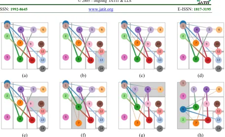
[image:7.612.94.550.60.338.2](e) (f) (g) (h)
2504 input is the rectangles generated from Squarified Treemap [32] that come in vertical (Ver) or horizontal (Hor) spans (rows) of rectangles, and the edges connecting these rectangles which are derived from the hierarchy tree. The rectangles within spans are ordered by being moved vertically or horizontally based on pulls from other rectangles. Figure 5 shows a treemap layout generated from a synthetic dataset, for the purpose of illustrating our method we only show the spans generated by the treemap. As the figure shows, the spans are:
spans[0] rects:[0, 1, 2, 3] dir:Ver spans[1] rects:[4, 5, 6] dir:Hor spans[2] rects:[7, 8] dir:Ver spans[3] rects:[9, 10] dir:Hor spans[4] rects:[11] dir:Ver spans[5] rects:[12] dir:Hor spans[6] rects:[13] dir:Ver spans[7] rects:[14] dir:Hor
Our ordering method, described in algorithm 1, works as follows: for each span of rectangles we want to find the order that minimizes the length of edges (distance) between rectangles in this span and all other rectangles. The order is found by first computing the total length of edges for a rectangle at each possible position in the span (lines: 13 - 16), then for each position subtracting the cost (either gain or loss) of moving the rectangle to a different position (lines: 17 - 18). Finally, for each position, the rectangle that minimizes the length cost is chosen (lines: 6 - 7). The complexity of algorithm 1 is O(tiEi), where ti and Ei are number of communities and edges, respectively, at pass i of the hierarchy tree.
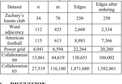
[image:8.612.109.278.243.343.2]Figure 5 (a) - (h) shows a sequence of ordering the rectangles in the 8 spans generated by the treemap. The span that is being ordered is highlighted with a light gray color. The total edges length is reduced from 19,765 to 14,661. Our method does not intrinsically target the number of intersections between edges however, practically, the reduction in edges length almost always leads to a reduction in the number of intersections, from 339 to 292 in our example. In table 1, we report the results of our experiments conducted on real datasets which are commonly used in the literature. Our results show 10% to 15% reduction in the total length of edges between communities leading to a less cluttered view.
Table 1: Length Of Edges Before And After Ordering Treemap Layout
Dataset n m Edges Edges after ordering Zachary’s
karata club 34 78 250 250
Word
adjacency 112 425 2,668 2,334
American
football 115 613 8,983 7,366
Power grid 4,941 6,594 22,264 20,260 Collaboration
99 13,861 44,619 130,651 104,002 Collaboration
03 27,519 116,180 1,871,680 1,582,861
6. DISCUSSION
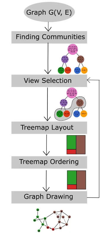
The main steps that are taken by our approach are summarized in figure 6. The visual output of each step is shown right below it. The input is a graph of nodes and edges that is likely to have communities; it can be undirected or directed graph. The graph size does not impose any restrictions on the system behavior, however, large graphs, that have hundreds of thousands of nodes and edges, can take hours to find communities [16]. The good news is that it only needs to be computed once and it can possibly carried out offline and then fed to the system. As the graph shows, in the first step, communities are generated at different resolution levels and the hierarchy tree is built. The
Algorithm 1 Ordering Treemap
1: forall s ∈ spans do
2: if s.rects:length == 1 then
3: continue
4: forall r ∈ s.rects do
5: lens[r] = LengthCost(r, s) 6: forall r ∈ s.rects do
7: r.center = min(lens[r]) 8:
9: functionLengthCost(r; s)
10: Output: Array of costs of links length of 11: positioning r at the center of all rects of s 12:
13: forall pos ∈ s.rects do
14: forall l ∈ r.links do
15: link distance when r is at pos:center
16: lens[pos:center] += distance(l; pos:center) 17: for i = 0; s:rects:length - 1 do
18: for j = i + 1, s.rects:length - 1 do
[image:8.612.314.522.411.555.2]ISSN: 1992-8645 www.jatit.org E-ISSN: 1817-3195
2505 communities found, by definition, satisfy property (1). This step is carried out only once while the remaining steps are performed repeatedly based on user interaction. In view selection, the user gets to select what level of details to include in the generated graph. The user can interactively change his selection seeking more or less details. Once the communities have been selected they are sent to the treemap layout. The treemap layout determines the gravity centers used for attracting and positioning communities, thus, emphasizing properties (2), (3), and (5). A reordering of treemap is applied to bring closer those communities that have high number edges between them and therefore encouraging property (4).
[image:9.612.330.502.94.485.2]In the last step, the graph is drawn using a force-layout model. The graph drawing represents the performance bottle neck of the approach as it takes O(VlogV) per iteration which renders it intractable for large graphs. Luckily, the user can consult with the hierarchy tree view to include only nodes of interest leading to fewer nodes being drawn. In our approach, the force calculation is modified to include the gravitational force that is exerted to attract nodes within communities closer to each other. In practice, the additional force enhances the performance causing the system to reach a local minima faster. Table 2 reports the number of iterations without and with gravitational force required for the system to stabilize. The experiments are executed 100 times and the average numbers of iterations are reported in the table.
Table 2: Number Of Iterations Required By The Force-Layout Model Without And
With Gravitational Forces
Dataset Iterations
Iterations with gravitational
force Zachary’s karata club
210 155
Word adjacency 288 178
American football 176 121
Power grid 70 39
Collaboration 99 65 50
Collaboration03
62 43
Figure 6: The Main Steps Of Our Approach
[image:9.612.100.290.509.683.2]2506
communities (out of 4) at the second level of the hierarchy tree and 12 leaf communities that are the children of the fourth communities from the higher level. The view represents an example of overview+details capabilities through which users can interactively explore the view investigating and seeking interesting patterns in the data.
7. CONCLUSION
We have incorporated refinements to the visual layout of graph community structure in order to satisfy desirable visual properties that aim at enhancing the perception of communities and support the investigation of their common features. The proposed approach has been tested on real datasets of medium sizes and has shown to effectively support separation of community regions and reduction of view clutter. Furthermore, the refinement in force calculation has been shown to improve the overall performance of the system.
REFRENCES:
[1] Newman ME. The structure of scientific collaboration networks. Proceedings of the National Academy of Sciences 2001;98(2):404–9.
[2] Ravasz E, Somera AL, Mongru DA, Oltvai ZN, Barab´asi AL. Hierarchical organization of modularity in metabolic networks. Science 2002;297(5586):1551–5.
[3] Jeong H, Tombor B, Albert R, Oltvai ZN, Barabasi AL. The large-scale organization of metabolic networks. Nature 2000;407(6804):651–4.
[4] Arenas A, Danon L, Diaz-Guilera A, Gleiser PM, Guimera R. Community analysis in social networks. The European Physical Journal B 2004;38(2):373–80.
[5] Schaeffer SE. Survey: Graph clustering. Comput Sci Rev 2007;1(1):27– 64.
[6] Newman MEJ, Girvan M. Finding and evaluating community structure in networks. Phys Rev E 2004;69(2):026113.
[7] Herman I, Melanc¸on G, Marshall MS. Graph visualization and navigation in information visualization: A survey. IEEE Transactions on Visualization and Computer Graphics 2000;6(1):24–43.
[8] Hu Y, Shi L. Visualizing large graphs. Wiley Interdisciplinary Reviews: Computational Statistics 2015;7(2):115–36.
(a)
(b)
[image:10.612.98.523.69.707.2](c)
Figure 7: Results Of Power Grid Dataset [36]. (A) Results Using Traditional Graph Drawing (B) Results Using Our Approach On A View Selection Of 37 Leaf Communities (C) View Selection Of 2 Levels That
ISSN: 1992-8645 www.jatit.org E-ISSN: 1817-3195
2507 [9] Eades P, Feng QW. Multilevel visualization
of clustered graphs. In: International Symposium on Graph Drawing. Springer; 1996, p. 101–12.
[10] Heer J, Boyd D. Vizster: Visualizing online social networks. In: Information Visualization, 2005. INFOVIS 2005. IEEE Symposium on. IEEE;2005, p. 32–9.
[11] Di Giacomo E, Didimo W, Grilli L, Liotta G. Graph visualization techniques for web clustering engines. IEEE Transactions on Visualization and Computer Graphics 2007;13(2).
[12] Quigley A, Eades P. Fade: Graph drawing, clustering, and visual abstraction. In: Proceedings of the 8th International Symposium on Graph Drawing. GD ’00; London, UK, UK: Springer-Verlag; 2001, p. 197–210.
[13] Shi L, Cao N, Liu S, Qian W, Tan L, Wang G, et al. Himap: Adaptive visualization of large-scale online social networks. In: Proceedings of the 2009 IEEE Pacific Visualization Symposium. PACIFICVIS ’09; Washington, DC, USA: IEEE Computer Society; 2009, p. 41–8.
[14] Abello J, van Ham F, Krishnan N. Ask-graphview: A large scale graph visualization system. IEEE Transactions on Visualization and Computer Graphics 2006;12(5):669–76. [15] Jonker D, Langevin S, Giesbrecht D, Crouch
M, Kronenfeld N. Graph mapping: Multi-scale community visualization of massive graph data. Information Visualization 2016;:1473871616661195.
[16] Blondel VD, Guillaume JL, Lambiotte R, Lefebvre E. Fast unfolding of communities in large networks. Journal of Statistical Mechanics: Theory and Experiment 2008;2008(10):P10008.
[17] Shneiderman B. Tree visualization with tree-maps: 2-d space-filling approach. ACM Trans Graph 1992;11(1):92–9.
[18] Muelder C, Ma KL. Rapid graph layout using space filling curves. IEEE Transactions on Visualization and Computer Graphics 2008;14(6).
[19] Holten D. Hierarchical edge bundles: Visualization of adjacency relations in hierarchical data. IEEE Transactions on Visualization and Computer Graphics 2006;12(5):741–8.
[20] Holten D, VanWijk JJ. Force-directed edge bundling for graph visualization. In: Computer graphics forum; vol. 28. Wiley Online Library; 2009, p. 983–90.
[21] Muelder C, Ma KL. A treemap based method for rapid layout of large graphs. In: Visualization Symposium, 2008. PacificVIS’08. IEEE Pacific. IEEE; 2008, p. 231–8.
[22] Fekete J, Wang D, Dang N, Aris A, Plaisant C. Interactive poster: Overlaying graph links on treemaps. In: In Proceedings of the IEEE Symposium on Information Visualization Conference Compendium. 2003,.
[23] Newman ME. Fast algorithm for detecting community structure in networks. Physical review E 2004;69(6):066133.
[24] Newman ME. Modularity and community structure in networks. Proceedings of the national academy of sciences 2006;103(23):8577–82.
[25] Newman MEJ. Finding community structure in networks using the eigenvectors of matrices. Phys Rev E 2006;74:036104. [26] Duch J, Arenas A. Community detection in
complex networks using extremal optimization. Physical review E 2005;72(2):027104.
[27] Brandes U, Delling D, Gaertler M, Goerke R, Hoefer M, Nikoloski Z, et al. Maximizing modularity is hard. 2006.
[28] Fruchterman TMJ, Reingold EM. Graph drawing by force-directed placement. Softw Pract Exper 1991;21(11):1129–64.
[29] Bender EA, Canfield E. The asymptotic number of labeled graphs with given degree sequences. Journal of Combinatorial Theory, Series A 1978;24(3):296–307.
[30] Molloy M, Reed B. A critical point for random graphs with a given degree sequence. Random Struct Algorithms 1995;6(2/3):161–79.
[31] Zachary W. An information flow model for conflict and fission in small groups. Journal of Anthropological Research 1977;33:452– 73.
[32] Bruls M, Huizing K, van Wijk J. Squarified treemaps. In: Proc. of Joint Eurographics and IEEE TCVG Symp. on Visualization (TCVG 2000). IEEE Press; 2000, p. 33–42.
2508 [34] Girvan M, Newman ME. Community
structure in social and biological networks. Proceedings of the national academy of sciences 2002;99(12):7821–6.
[35] Shneiderman B, Wattenberg M. Ordered treemap layouts. In: Proceedings of the IEEE Symposium on Information Visualization 2001 (INFOVIS’ 01). INFOVIS ’01;Washington, DC, USA: IEEE Computer Society; 2001, p. 73–.
![Figure 1: An Illustrative Example Of Blondel's Approach [16]. (A) And (B) Show Phase 1 And Phase 2 Of Pass 1, Respectively, (C) Shows The Resulting Graph Of Pass 2, (D) Presents The Hierarchy Tree Built During The Process](https://thumb-us.123doks.com/thumbv2/123dok_us/8906814.957208/4.612.96.518.65.223/illustrative-example-approach-respectively-resulting-presents-hierarchy-process.webp)
![Figure 2: Zachary’s Karata Club Dataset [31]. (A) View Of The Original Graph Showing The Two Communities, (B) Circos View Of Edge Density In (A), (C) View Of The Random Graph Generated Using The Configuration Model, And (D) Circos View Of Edge Density Of R](https://thumb-us.123doks.com/thumbv2/123dok_us/8906814.957208/5.612.99.509.59.479/zachary-dataset-original-communities-density-generated-configuration-density.webp)
![Figure 3: Graph Layout Of Word Adjacencies Dataset [25]. (A) Original View Where Convex Hulls Of Community](https://thumb-us.123doks.com/thumbv2/123dok_us/8906814.957208/6.612.90.298.424.629/figure-graph-layout-adjacencies-dataset-original-convex-community.webp)
![Figure 7: Results Of Power Grid Dataset [36]. (A)](https://thumb-us.123doks.com/thumbv2/123dok_us/8906814.957208/10.612.98.523.69.707/figure-results-power-grid-dataset.webp)
