2942
QUERY OPTIMIZATION ON DISTRIBUTED HEALTH
DATABASE DBD FOR SUPPORTING DATA CENTER WITH
MATERIALIZED VIEW AND MINIMIZING ATTRIBUTE
INVOLVEMENT
SUDARYANTO#1, SLAMET SUDARYANTO N#2, FIKRI B#3, MARYANI S*4
#Faculty of Computer Science, Dian Nuswantoro University
Central Java, Indonesia
1[email protected], 2[email protected], 3[email protected]
*Faculty of Health, Dian Nuswantoro University
Central Java, Indonesia 4[email protected]
ABSTRACT
The integration of data from various sources is an important step to establish a data warehouse in order to form a decision support application. The problem is how to find and integrate optimally the various data from distributed heterogeneous database sources. The heterogeneity of data sources has a number of factors, including storing databases in various formats, using different software and hardware for database storage systems, designing in different data semantic models. There are currently two approaches to data integration: Global as View (GAV) and Local as View (LAV), but both have performance limitations and need to find ways to optimize them. Some of the key factors to be considered in making data integration optimal are query response time and understanding of structure of the data source (source schema). Query response time plays an important role as timely access to information and it is the basic requirement of successful business application. A data warehouse uses multiple materialized views (MV) to efficiently process a given set of queries. Query process requires important attention especially in source schema, because the results of cost-based query processes (access costs and stored costs) are influenced by the involvement of the number of attributes and sites visited. This paper gives the results of proposed minimize attribute involvement based MV selection algorithm for query processing. First, select MV by clustering the workload of the query. A query is decomposed into a sub-query that requires operations on a separate database and can determine the exact order of site access. From the query process query sequence, the operating costs for the query process will be minimal. When a query process in a distributed database occurs, query operations will look for data from various attributes in a scattered database table, whereas query processes often do not require all the attributes of the tables. Therefore, to optimize the query requires minimum operating cost requests (access costs and stored costs) by separating the use of
unnecessary attributes. Second, a join index that is specifically adapted to the multidimensional architecture of warehouses. It eliminates join operations while preserving the information contained in the original warehouse. This approach can also to minimize the cost of the request in addition to separating attributes that are not required by the request, thereby reducing the amount of time store and access. In the separation of attributes, attributes are shared indiscriminately, because otherwise they will result in greater access fees and ultimately reduce the performance of the query process. To perform such attribute separation can be done by Vertical Fragmentation method. To validate this study, we measured response times from a set of decision support Queries through DBD data warehouse, with and without using our optimization techniques. Our experimental results show their efficiency, even when queries are complex and the data is relatively large.
.Keywords: Global as View, Local as View, Materialized View, Access Costs , Stored Costs, Data
Warehouse
1. INTRODUCTION
The information produced by an application comes from a lot of data that is local, not uniform and autonomous as a reference in
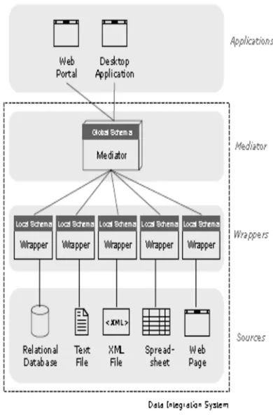
2943 databases. It takes extra effort to make the function of integrating or integrating various heterogeneous sources of data. The first step that must be done in data integration is to retrieve data from various different sources, then understand the relationship of each data source (source schema) with the global scheme. Accommodate differences in structure and values and the potential for inconsistencies from local schemes to global schemes. The process of data integration and exchange between data requires the transformation of local data structures into schemes, namely the transformation of source schemes into target schemes that have different data structures. The process of transforming a local scheme into a target scheme is usually called schema mapping. Mediators are needed as a concept of integration architecture between different schema sources [7]. The wrapping function is used to wrap the information container and model it into the schema source. The mediator function is used to maintain the global scheme and mapping between local and schematic global schemes. When the user queries all objects related to the global scheme, the mediator will use the reformulation-query procedure to translate the query into executable sub-queries from all the schema sources involved in the query process and then reassemble the answers from each source of the scheme to be combined further to answer the query. At present various approaches and categories can be used to integrate federations or multi-database systems [11]. Currently in integrating data in the global scheme there are three categories of languages in expressing correspondence, namely: Global as View (GAV), Local as View (LAV), Global Local as View (GLAV), Both as View (BAV) along with theory and related system [8], [9]. From the literature the Query processing algorithm for LAV describes a data integration system that describes and adopts the GAV query integration system and the query process. In the GAV approach, reforming queries can reduce the application of rules to be simple (display of standard execution on a regular database). However, the mapping process in the global GAV scheme requires a synchronization process between the global scheme and the local scheme as the source of the scheme. Especially if there is a change or addition from the source scheme as a source of information from GAV. In large-scale applications LAV is easier to manage than GAV because the DBA makes a global scheme regardless of the source scheme. When there is a need for a new scheme as a data source, the DBA only adjusts the
[image:2.612.332.527.254.550.2]description of the source scheme which describes the relationship of the data source as a form of the global scheme. So that the automation of reformulation queries in LAV has complex exponential times. This problem is directly related to the query process and the definition of source schemes. If LAV is used as a Data Center support, LAV has a low query process performance when users often request complex queries. In order for the data center to have a better performance, the number of engagement attributes from LAV must be evaluated.
Fig 1. View Based Data (VBD) Integration System
2. RELATED WORK
2944 model we need some special methods that are different from the data source level autonomy. For example, a method by Calibration [15] estimates the coefficients of the generic cost model for each type of relational data source. This calibration needs to know the access method used by the source. This method is extended to object-oriented databases by [16]. If this procedure of the abrasion can’t be processed because of the data source constraints, the sampling method proposed in [17] can be derived cost model for each type of query. The query classification in [17] is based on a set of common rules adopted by many people DBMSs. When no implementation algorithm and formation fees are available, we can use the method described in [2], where the estimated cost of the new request is based on the history of questions evaluated thus far. Specifically, for semi-structured data sources, [1] proposed two techniques to estimate simple XML selectivity of a path expression over complex, large-scale XML data as done by an XML-scale XML application. [18] describes cost-based query optimizers in DBMS for XML- based on data that support expressive query language. [19] proposed an approach to using a new statistical learning technique called "regression transformation" rather than a detailed analytical model to predict the overall cost for XML-based data sources.
[20] proposed a mediation system called DISCO, based on a global-as-view (GV) approach. DISCO mediator is distributed operations executed at the data source level (wrapper) and operations are conducted at the mediator level. The DISCO data model is based on the ODMG standard. Disco uses a cost-based optimization approach that combines the general cost model with the specific cost information exported by the wrapper. The data source interface is defined using a subset of expanded CORBA IDL with the cardinalities section for the data source statistics and the cost formula section for a custom formula. This section defines the cost-communication languages that are appropriate for an object-oriented environment but not generic. Other mediation systems with cost-based demand optimization include Garlic [21], Hermes [22], Ariadne [3], etc. However, none of the above mentioned solutions have overcome the overall cost estimation problem in a semi-structured environment integrating heterogeneous data sources.
In [4] the authors overcame the notion that server data stores can’t communicate with each other and propose models that divide data over different
fragments. The main difference between the work of previous researchers and the work proposed in this paper is that we consider evaluating the cost of the query during the fragmentation process and overcoming the fragmentation computing problem it minimizes the cost of such a request. An important aspect that needs to be emphasized in cost-based query optimizer is how to explore the set of alternative execution plans as search space. In order to generate a new plan from the original then the mediator usually uses the rules of transformation and data mapping. The large number of rules and the involvement of many attributes will cause the exponential explosion of the query plan candidate. So it will directly require a search space containing the candidate's execution plan. This will result in inefficient use of search space resulting in high costs in the query process. For that needed a search strategy that can reduce the size of the search space that contains the candidate execution plan. In [18] the authors describe 3 important rules that are commonly used by most DBMS in generation planning: (1) Transformation by join order; (2) Avoid cross product join; (3) Avoid taking intermediate results as the inside operand of each join. Furthermore, commercial systems will use dynamic programming algorithms in generating candidate plans. [23] This algorithm performs a dynamic scan, a complete search that can build all alternative merging trees (choose 3 rules). By repeating on the number of relationships merged so far and removing the un-optimized trees.
3. METHODOLOGY
2945 system will transform the request into a sub-query stated in the local scheme of several independent data sources.
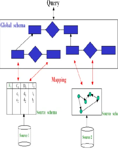
Fig 2. Mapping Data Integration System
Two main components that must be considered in conducting data integration, namely Integration Scheme and Query Processing. The integration of schemes can be directly related to how various local schemes can be combined into one global scheme directly. While query processing related to how queries can be answered by translating to one or several queries in the source database. There are four main approaches to data integration: Local as View (LAV), Global as View (GV), Global Local as View (GLAV) and Both as View (BAV). All of these approaches are not realized (virtual) where it uses a view definition to determine the mapping between local schemes and global schemes. The view definition is the result of a query for basic relations whose results are not stored in a data base (non materialized). Mapping is used to translate queries expressed in the global schema framework for sub-queries expressed in local schemes.
3.1 Conjunctive Queries and Datalog Notation.
In modeling and expressing view definitions and queries, datalog notation is needed [11,12]. Data integration is a triple relationship (G, {Si}, {Mi}), where G is the target of the global scheme or scheme, {Si} is the number n source schema and
{Mi} is mapping the number n sources for the target scheme. So for each source scheme Si is Mi from Si to T, 1≤ i ≤ n. The data integration system is a process of combining data that is in a different source {Si}. Mapping between local data sources or schemes and the global scheme as a data center is a set of statements:
1.
S => qG ,
2.
G => qS,
Intuitively, the first statement states that the concept is represented by view (query) qS as an S source scheme (LAV) in accordance with the concept defined by qG as a global scheme (GAV), and vice versa.
3.2 Mapping Schema Construction.
2946
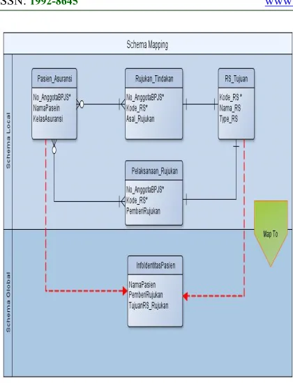
Fig 3. Mapping Local Schema to a Global Schema
If the input is not exactly the same as the source, here it is used to generate schema mapping, we give an inaccurate sample by leaving it "noisily contain" by some database examples. Formally it can define a relationship ("noisily contain") by a binary operator ≽, which returns the boolean value based on the desired error model. Using this operator we can say notifying a sample containing "noisily contain" as E iff t [A] ≽ E. Similarly we say that t contains E iff ƎA s.t. t [A] ≽ E. Then given tE = (E1, .. Em), we call T containing tE, iff ˅ i ∈ [m], t [Ai] ≽ Ei. Finally we can determine the target database Dt containing t E iff Ǝt ∈ Dt s.t contains tE. This underlying concept in defining sample searches is as follows: if the source database Ds is given and the sample tuples tE = (E1, ...., Em), in the search to find all M scheme mapping in such a way that the mapping results come from the source database M (schema mapping) from the database source (Ds) contains all database tuples from the tE source, then each result of the schema mapping is called a valid schema mapping model.
3.3 Process Query Translation.
The query process is directly related to several queries (Q), such as if there are two pairs of source databases (Ss) from different structures such as (Ds) containing local schemes with multiple relations (n relations R1 ... Rn). If there are
questions that involve all local schemes from different Ds source database pairs, then it will prepare several processes from the query translation, such as semantic translation queries, advanced query translations (tree pattern backgrounds, joined translation tree patterns), and backward query translations. For each candidate set V (view) of the selected cover, the general commands used to select are:
Select attributes in (View)
[image:5.612.93.303.78.353.2]From source relations in the join path for (View) Where filter and join conditions from the join path
[image:5.612.321.539.243.674.2]Fig 4. Mapping Algorithm
2947 The documents that need to be considered as global data statements from source data are like "one fact in one place." The filter that is applied to global data is to minimize the data attribute of the source and complete global data needs. With this filter, we try to uphold these principles for the values chosen by the filter because our goal is schema mapping rather than schema design. The application of this filter allows users to change the arrangement of source attributes in order to fulfill the desired global information. For example, in publishing information for a "What-If" scenario, users can combine attributes cross or break attributes until they can evaluate all possibilities. To obtain information (target schemes) from various source schemes, we use these principles to encourage initial mapping to the maximum extent possible. Users can block target data from mapping and decide whether to modify the mapping so that the tree mapping process becomes a reference for querying with certain attributes and filters. If applied to the tree mapping of the image above then the additional correspondence command is:
F_1 : patien(id_pasien) rs_rujuka(id_pasien)
F_2 : patien(dok_keluarga)
r-rujuka(dok_keluarga)
F_3 : patien(dok_rujukan) rs_rujuka(do_rujukan)
F_4 : patien(rs_rujukan) rs_rujuka(rs_rujukan)
F_5 : pasien(id_pasien) rs_rujuka(id_pasien)
F_6 : pasien(d_rujukan) rs_rujuka(dok_rujukan)
F_7 : pasien(dok_rujukan) rs_rujuka(dok_rujuka)
F_8 : pasien(r_rujukan) rs_rujuka(nama_rs)
select pt.id_pasien, pt.dok_keluarga, pt.dok_rujukan, ps.id_pasien, ps.nama_rs from patient pt, pasien ps
where pt.id_pasien=ps.id_pasien union all
select null as dok_keluarga, ps.id_pasien , ps.dok_rujukan*pt.d_rujukan, null as pasien_reguler
from patient pt, pasien ps where pt.id_pasien=ps.id_pasien
create view t_rujukan (id_pasien, dok_keluarga, nama_kasus, nama_rs) as
select f1(s1, id_pasien, dok_keluarga), f2 (s2,dok_rujukan, fast_rujukan, rs_rujukan) from s1,s2
where s1.id_pasien=s2.id_pasien union
select f2(s2, id_pasien, null, rs_rujukan)
3.4 Query Workload Analysis.
The workload of the query process we consider is a set of selection, join and aggregation queries.
This first step consists in extracting from the workload representative attributes for each query. We mean by representative attributes those are present in Where (selection predicate attributes)
and Group by clauses. We store the relationships
between workload queries and the extracted attributes in a so-called “query-attribute” matrix. Matrix lines are queries and columns are extracted attributes. A query qi is then seen as a line in the
matrix that is composed of cells corresponding to representative attributes. The general term qij of
this matrix is set to one if extracted attribute ai is
present in query qi , and to zero otherwise. This
matrix represents our clustering context.
3.5 View and Materialized View (MV).
View is a virtual table that does not have to exist in the database, but can be generated based on requests from certain users when desired [2]. View is a dynamic process of one or more operations performed on the base table to generate another table. View is dynamic, meaning that if the base table changes, then the view directly shows the change. The purpose of view creation is:
1. Provide a flexible and good security mechanism by hiding part of the database of users. 2. Allows users to access data in a customized manner, so that the same data can be viewed by different users in different ways at the same time.
3. Simplify complex operations on the base table.
2948 physical sequence of data in the table [7]. Clustered index stores rows of data in tables based on key values. While non-clustered index store pointer to table data as part of key index.
Using indexes to improve query performance is not a new concept, but indexed view provides additional performance benefits not found in the standard index. Indexed view can improve query performance in the following ways:
1. Aggregation can be pre-computed and stored in the index to minimize the high computation of query execution.
2. tables can be pre-joined and the resulting data stored.
3. combinations of join and aggregation can be stored
Aggregation and join are often the right candidates for indexed view. A query can be a candidate of the indexed view if it takes significant time and large amount of data to get the query results quickly. Indexed view will work very well when the data is relatively static or rarely updated. While the transactional environment is not suitable for indexed view. Some application systems that can implement indexed views are: decision support workloads, data marts, data warehouses, online analytical processing (OLAP) databases, data mining.
3.6 Proposed Algorithm.
In a distributed database environment the data source is derived from various nodes. It might happen that the same copy of the database exists on multiple nodes. Therefore query execution on each and every node will be inconvenient and time consuming in a distributed environment. This becomes even more complicated when materialized views are made for distributed databases. To minimize the storage of query results and increase the query response time of the materialized views (MV), the selection of attribute involvement according to the query access requirement is very significant for query execution. Two proposed algorithms are presented to address the issue of query access fees and the cost of clustered index storage of MV underlying the proposed query optimization query. The first algorithm is for generating and selecting attribute attributes required by MV. Tree-based approaches are used to create and maintain MV. Initially all records are arranged in ascending order of their key values. Then the middle note is selected as the root of the tree element. The record is then divided up until the threshold does not reach so that the tree leaf should contain the number of records that
will be available in the materialized view. Then the materialized view is created for each leaf node, indirectly each leaf representing a materialized view that must be created and maintained. The materialized view is selected on request. It's a note whose request meant the view materialized and only that record would be selected for processing. This minimizes total execution time for query processing. That selective approach can also be used to create a materialized view that minimizes storage costs. The second algorithm is for the selection of nodes. This algorithm decides the nodes in the distribution of the environment to which the realized view must be created, updated or maintained. The random walk algorithm is used as the basis for designing node selection algorithm and protocol gossip is used to find the best node set. In the following algorithm, recordings are initially compiled in ascending order of their key values using set (R). Then the middle note is selected as the root node. For each note on the available node, if the threshold is less than the number of records in the leaf node then split again the records in the same set; if not, make the tangible look for the next note available in the leaf node & add the materialized view in the view set.
3.7 Cost Analysis
The total cost for materializing views can computed using the following strategy. The proposed algorithm considers query processing cost (for selection, aggregation and joining), view maintenance cost, storage cost, net benefit and storage effectiveness for computing the total cost. The cost is calculated in terms of block size B. The query processing cost in terms of block access is equal to size of materialized view Vi. [14,19].
CB (Vi) = S(Vi)
The query cost involving the joining of n dimensional tables with view Vi is given by
Cj(Vd1, Vd2,…, Vdn , Vi) = (S(Vd1) + S(Vd1) *S(Vi))
+ (S(Vd2) + S(Vd2) *S(Vi)) +…..+ (S(Vdn) +
S(Vdn)* S(Vi))
To process user’s query qi, which requires not only selection and aggregation of the view, but also the joining of view with other dimension tables, the query cost Cq(qi) is given by
Cq(Vi) = CB (Vi) + Cj(Vd1, Vd2,…, Vdn , Vi) = S(Vi) + (S(Vd1) + S(Vd1) *S(Vi)) + (S(Vd2) + S(Vd2) *S(Vi)) + ….+ (S(Vdn) + S(Vdn) *S(Vi)).
Thus the total Query cost Total (Cqr) for
2949 Total =(Cqr)= fqt ∗ Cq qt
The re-computation of each view requires selection and aggregation from its ancestor view Vai , and their joining with n dimension tables.
Therefore the maintenance cost is given by
Cm(Vi) = CB (Vai) + Cj(Vd1, Vd2,…, Vdn , Vai) = S(Vi) + (S(Vd1) + S(Vd1) *S(Vai)) + (S(Vd2) + S(Vd2) *S(Vai)) + …. + (S(Vdn) + S(Vdn) *S(Vai))
The cost for storing materialized views depends on the availability of hard disk space. The storage factor U represents the estimated ratio of the storage capacity required by the data warehouse to the availability of hard disk space it is given by
U = (Total (Cstore) + (1+Q) * Y *Sa) / Total
available storage capacity
Where ‘(1+Q) * Y * Sa’ estimates the total increase in storage capacity for accommodation of new data during processing or creation of materialized views. Here Q is the estimated increase rate in data volume per year within data warehouse, Y is the estimated processing cycle of the data warehouse, and Sa is the storage space required to store added new data and their
materialized data. The storage cost of view in terms of data block B is given by
Cstore (Vi) = U * S (Vi)
In most of the today’s systems storage space doesn’t matter because large amount of hard disk space is available with less prize so in proposed algorithm implementation the value of
U=1. Therefore the total storage cost is calculated as
Cstore (Vi) = S(Vi)
4 DISCUSSION AND EXPERIMENT
RESULT
4.1 Global As View (GAV) to Materialized
View.
Experimental results were performed on different health DBD databases. Between DBD databases stored in different locations will be the data source of the data center (data warehouse). Two storage location locations are used to experiment with data integration using the proposed method, ie from GAV as an all-virtual views method to all
modified materialized views. The step starts first by creating a unique cluster index that is appropriate to save the view results from GAV. When creating GAV attributes of local schema in selection or in filter first. The goal is to minimize attribute involvement when forming GAV, thus minimizing the capacity of storage space when creating a materialized view (index view from GAV). Then use tree-based approaches used to create and maintain MV. To measure the performance of the proposed method, the authors only measure from the performance elements Query Processing Cost and Storage Cost. In the experiment used 20 queries. Each refers to the view of the local schema and index view in the global schema. Each query is grouped into query join, aggregation query, and mixed query (query join & aggregation query). After measuring the query processing cost and storage cost the next step is to compare and measure the increase in query processing time as the average query response time in milliseconds (ms).
2950
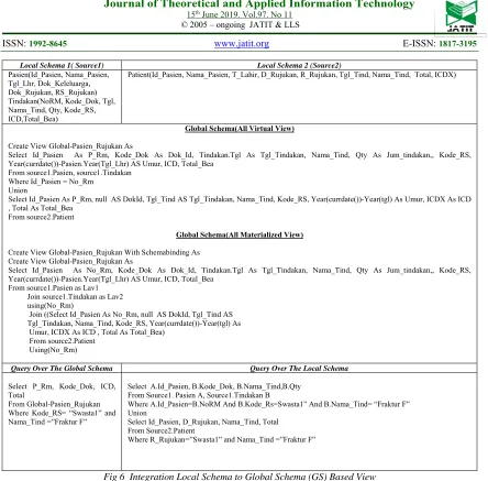
Local Schema 1( Source1) Local Schema 2 (Source2)
Pasien(Id_Pasien, Nama_Pasien, Tgl_Lhr, Dok_Keleluarga, Dok_Rujukan, RS_Rujukan) Tindakan(NoRM, Kode_Dok, Tgl, Nama_Tind, Qty, Kode_RS, ICD,Total_Bea)
Patient(Id_Pasien, Nama_Pasien, T_Lahir, D_Rujukan, R_Rujukan, Tgl_Tind, Nama_Tind, Total, ICDX)
Global Schema(All Virtual View)
Create View Global-Pasien_Rujukan As
Select Id_Pasien As P_Rm, Kode_Dok As Dok_Id, Tindakan.Tgl As Tgl_Tindakan, Nama_Tind, Qty As Jum_tindakan,, Kode_RS, Year(currdate())-Pasien.Year(Tgl_Lhr) AS Umur, ICD, Total_Bea
From source1.Pasien, source1.Tindakan Where Id_Pasien = No_Rm Union
Select Id_Pasien As P_Rm, null AS DokId, Tgl_Tind AS Tgl_Tindakan, Nama_Tind, Kode_RS, Year(currdate())-Year(tgl) As Umur, ICDX As ICD , Total As Total_Bea
From source2.Patient
Global Schema(All Materialized View)
Create View Global-Pasien_Rujukan With Schemabinding As Create View Global-Pasien_Rujukan As
Select Id_Pasien As No_Rm, Kode_Dok As Dok_Id, Tindakan.Tgl As Tgl_Tindakan, Nama_Tind, Qty As Jum_tindakan,, Kode_RS, Year(currdate())-Pasien.Year(Tgl_Lhr) AS Umur, ICD, Total_Bea
From source1.Pasien as Lav1 Join source1.Tindakan as Lav2 using(No_Rm)
Join ((Select Id_Pasien As No_Rm, null AS DokId, Tgl_Tind AS Tgl_Tindakan, Nama_Tind, Kode_RS, Year(currdate())-Year(tgl) As Umur, ICDX As ICD , Total As Total_Bea)
From source2.Patient Using(No_Rm)
Query Over The Global Schema Query Over The Local Schema
Select P_Rm, Kode_Dok, ICD, Total
From Global-Pasien_Rujukan Where Kode_RS= “Swasta1” and Nama_Tind =”Fraktur F”
Select A.Id_Pasien, B.Kode_Dok, B.Nama_Tind,B.Qty From Source1. Pasien A, Source1.Tindakan B
Where A.Id_Pasien=B.NoRM And B.Kode_Rs=Swasta1” And B.Nama_Tind= “Fraktur F” Union
Select Id_Pasien, D_Rujukan, Nama_Tind, Total From Source2.Patient
[image:9.612.88.532.39.476.2]Where R_Rujukan=”Swasta1” and Nama_Tind =”Fraktur F”
Fig 6 Integration Local Schema to Global Schema (GS) Based View
4.2Answering Query (Using Materialized
View).
There are several things that pertain to the query process that must be considered and have an effect on the effectiveness of query answering in the data integration schema. Some things to watch out for are: constraint / integrity constraints in the global schema, permitted classes in the mapping and query classes in the mapping. The treatment algorithm will be different between GAV with constraint and GAV without constraint. For GAV without constraint is the simplest case in answering query. This model is also considered to be the first order query in the mapping. Its view is exact so it can be proved that there is one global database as a target that is mapped from legal data sources. In GAV without a global database constraint derived from the source schema where the display's existence is calculated by using the display definition to map it. The answer to the query, the query user is calculated by evaluating
the query through the global database. Likewise to modify the query, the user can easily be able to obtain an equivalent query that can be executed based on the source. This can be done easily after the ongoing strategy where each atom is above View (V) where V is the symbol of the relation in the global schema replaced by a query corresponding to the GAV mapping.
2951 equivalent question if the source attribute is directly related to the needs of the target scheme. Suppose that is a database scheme and V is a set view of T.Query P can be expanded by using the inner view V, denoted Pexp, obtained from P by
replacing all views in P with the corresponding base relation. Queries on P on T are called Q query rewriting and are directly related to V if P uses only views in V, and Pexp is in Q as a query. Thus P is called a rewrite query and the equivalent Q that uses V if Pexp and Q are equivalent to queries.
Pasien(Id_Pasien, Nama_Pasien, Tgl_Lhr, Dok_Keleluarga, Dok_Rujukan, RS_Rujukan) Tindakan(NoRM, Kode_Dok, Tgl, Nama_Tind, Qty, Kode_RS, ICD,Total_Bea)
Dokter(Kode_Dok, Nama, Spesialisasi)
Query Q1,
Select D.Nama, Total_Bea
From Pasien P, Tindakan T, Dokter D Where P.Id_Pasien=T.RoRM AND
T.Kode_Dok=D.kode_Dok And Dok_Keluarga =” dr. jennar”
Queries wants to display the attribute data of the doctor's name to find out the total cost of the patients treated by the family doctor dr. jennar. Queries and views are often written with conjunctions, so the query can be rewritten as :
Q1(T,G) : -Pasien(P, N, joko), Tindakan(P, D, G), Dokter(D, T, Q)
In constant arguments like the lowercase letters in the "joko" sentence are the arguments for constants, while large lettered arguments (like "P") for variables. The symbol ": -" as the body of the query command body, which has a sub-goal with an extended body part as a whole body relationship. The small letter "joko" as a constant in the first sub-destination represents the selection condition. Variable S is owned by the first two sub-regions. This region represents the combination of patient relationships and actions in the patient-id_pasien attribute. The T and G variables as query heads (on the left side of the ": -" notation, represent the final projected attribute.) The results of the views that have been defined from the base table are:
Views :
V1(I, N, Dk, K, Nt,Q):- Pasien( I, N, Dk), Tindakan(No, K, Nt, Q)
V2(No, K,Nt,M,Q):- Tindakan(No, K, Nt, Q), Dokter(K, M,S)
So the SQL command to define view 1 is as follows
CREATE View V1 As
Select P.Id_Pasien, P.Nama_pasien,
P.Dok_keluarga, T.Kode_Dok,T.Nama_Tind, T.Qty
From Pasien P, Tindakan T Where P.Id_Paseien=T.NoRM
This view is a combination of the patient's relationship with medical action. This is also the case in View V2 is a combination of medical measures (treatment size and doctor), except the value and value attributes are dropped on the final result. Here are the results of the q1 writing query using 2 View.
Answer(N,Nt):-V1(I, N,joko, K, Nt), V2(No, K, N)
This view is a combination (natural) of the relationship between patients and medical action. Also at view V2 is a combination (natural) of the relationship of medical action and family doctor, except that the value attribute is dropped on the final result. The query can be rewritten q1 using two views.
Answer (M,Nt) :- pasien (I, N, joko, K, Nt), Tindakan(No,K,Nt), Tindakan (N,K,Nt’), Dokter (K, M, S’)
Nt 'and S' are new variables introduced during substitution. This extension is equivalent to a query, so rewriting is equivalent (relevant) to the previous query. If it involves a V2 view and found the conditions for selecting a new attribute then the definition j is as follows:
V2’(I,K,M):-Tindakan ( S, K, Nt), Dokter ( K, M, internis )
If when defining V2 there is a selection condition again in the quarter attribute, then the view will be defined as:
Answer(M,Nt):-V1(I,N,joko,K, Nt), V2’(I,K,M)
Attribute description:
2952 Global View Mapping is very suitable for relatively stable data sources, global view mapping will be difficult if there are new data sources that change frequently and are uncertain. So it requires an algorithm that can dynamically pair the schemes that will be mapped. GAV Fitting The algorithm of the source schema attribute to the global schema attribute occurs in three stages.
[image:11.612.317.528.84.704.2]Fig 7. Desain Central Data Warehouse Architecture
Fig 8. Data Staging Process
4.3 Experiment Result.
[image:11.612.94.303.190.325.2]Based on the results of experiments that have been done on 20 queries that each refer to the view and index view that has been in the filter. There is a difference of response time (answering query) to each query group. Here is a graph table showing the response time difference.
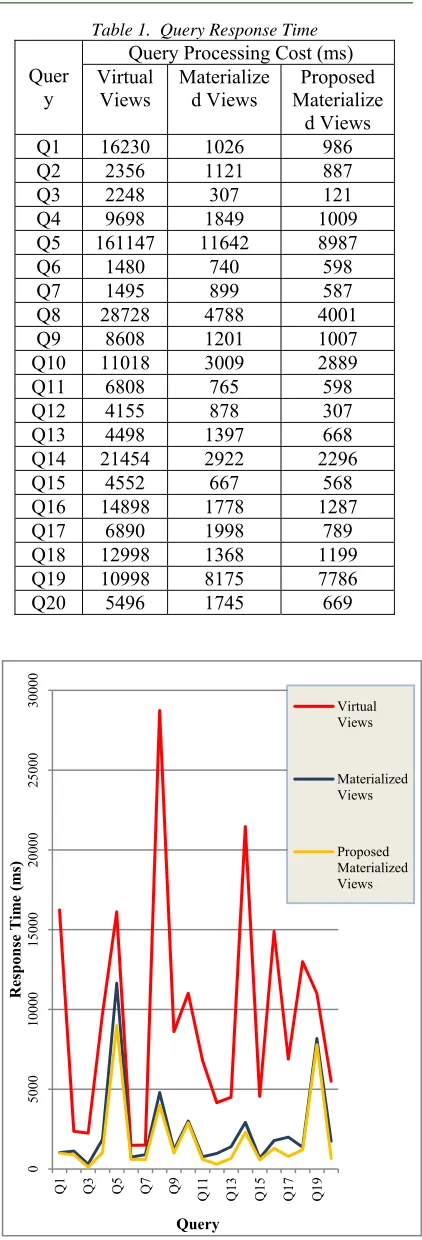
Table 1. Query Response Time
Quer y
Query Processing Cost (ms) Virtual
Views Materialized Views MaterializeProposed d Views Q1 16230 1026 986 Q2 2356 1121 887 Q3 2248 307 121 Q4 9698 1849 1009 Q5 161147 11642 8987 Q6 1480 740 598 Q7 1495 899 587 Q8 28728 4788 4001 Q9 8608 1201 1007 Q10 11018 3009 2889 Q11 6808 765 598 Q12 4155 878 307 Q13 4498 1397 668 Q14 21454 2922 2296 Q15 4552 667 568 Q16 14898 1778 1287 Q17 6890 1998 789 Q18 12998 1368 1199 Q19 10998 8175 7786 Q20 5496 1745 669
Fig 9. Graph Comparison Of Query Processing Cost
0
50
00
10
000
15
000
20
000
25
000
30
000
Q1 Q3 Q5 Q7 Q9 Q11 Q13 Q15 Q17 Q19
Response Tim
e
(m
s)
Query
Virtual Views
Materialized Views
[image:11.612.96.303.362.529.2]2953 Based on the result of the average response test of the experiment between the materialized view with the proposed method, it can be known the cost of the magnitude of the approach of the query response time generated between the two approaches. Performance measurement is done by comparison ratio of query response time between both methods. So as to obtain acceleration or increased query response time as the cost of the query process.
Table 2. Performance Increased Execution Time By The Proposed Approach
Quer
y Number Of Record
s
Size (Bytes )
Query Workload
Analysis
Increase d Time
Q1 987 389
Query Join
104 % Q2 4660 339 126% Q3 3000 156 253% Q4 5564 450 54% Q5 19781 391 128% Q6 68991 433 123% Q7 9770 234 130% Q8 108085 143 119% Q9 793 233
Query Aggregatio
n
119% Q10 18009 335 104% Q11 4506 347 127% Q12 33984 231 123% Q13 45997 334 123% Q14 17009 761 78% Q15 121084 651 117% Q16 609 118
Query Aggregatio
n & Join
138% Q17 2093 443 126% Q18 8058 234 114% Q19 45607 189 104% Q20 159078 231 111%
From the results of experiment done can be obtained the result that the query with indexed view or materialized view has a faster execution time compared with virtual view. This happens on all types of queries. Table 2 shows that the use of indexed views can improve query performance in accessing data up to 253% faster than virtual views. Increased acceleration time occurs in the join query group.
Table 3. Query Response Time
Query
Storage Cost Virtual
Views Materialized Views Proposed Material Views Q1 0 1238 380 Q2 0 2416 654 Q3 0 1356 455 Q4 0 1177 319 Q5 0 1844 867 Q6 0 2730 790 Q7 0 1579 449 Q8 0 588 197 Q9 0 2445 865 Q10 0 2956 814 Q11 0 3099 998 Q12 0 1589 566 Q13 0 2803 851 Q14 0 997 486 Q15 0 1975 719 Q16 0 909 355 Q17 0 840 283 Q18 0 1123 616 Q19 0 658 339 Q20 0 769 509
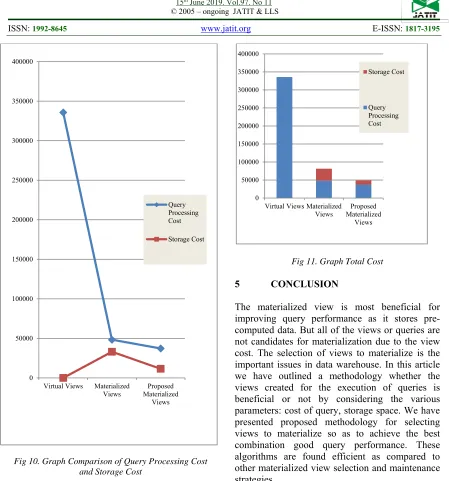
Table 4: The Query Processing and Storage cost for three Materialization Strategies
Strategy
Approach Processing Query Cost
Storage
Cost Total Cost
Virtual Views 335755 0 335755 Materialized
Views 48275 33091 81366 Proposed
Materialized Views
37239 11512 48751
2954
Fig 10. Graph Comparison of Query Processing Cost and Storage Cost
Fig 11. Graph Total Cost
5 CONCLUSION
The materialized view is most beneficial for improving query performance as it stores pre-computed data. But all of the views or queries are not candidates for materialization due to the view cost. The selection of views to materialize is the important issues in data warehouse. In this article we have outlined a methodology whether the views created for the execution of queries is beneficial or not by considering the various parameters: cost of query, storage space. We have presented proposed methodology for selecting views to materialize so as to achieve the best combination good query performance. These algorithms are found efficient as compared to other materialized view selection and maintenance strategies.
Based on the experiments conducted indexed view proven to improve query performance in accessing data significantly on distributed databases. After modifying the materialized view method by selecting the attribute involvement from the source schema, the indexed view as a materialized view may increase in performance compared to before it is modified. In this query process query efficiency test the author uses two cost parameters, namely Query Processing Cost and Storage Cost. At first the experiment was performed to record the response time query, in this experiment the proposed method had a faster response time. then performed piercing for storage cost, the result of the proposed method has a smaller storage cost. The proposed materialized view method proved to be faster than the old materialized view
0 50000 100000 150000 200000 250000 300000 350000 400000
Virtual Views Materialized
Views MaterializedProposed Views
Query Processing Cost
Storage Cost
0 50000 100000 150000 200000 250000 300000 350000 400000
Virtual Views Materialized
Views MaterializedProposed Views
Storage Cost
2955 (unmodified). Even the response time query results on the type of query join has a percentage increase in query processing can reach 253% faster than previous methods. To improve this research, the future can add cost maintenance parameter as an indicator of the efficiency of the query process with this materialized view modification method.
ACKNOWLEDGEMENTS
This research received full support and funding sponsorship from the Ministry of Research and Technology-Higher Education of the Republic of Indonesia. Planning, operational coordination and supervision are carried out by LLDIKTI Region VI of Central Java. The authors express their gratitude for their attention and guidance.
REFERENCES
[1] McBrien, Peter, and Alexandra Poulovassilis. "Data integration by bi-directional schema transformation rules." Data Engineering, 2003. Proceedings. 19th International
Conference on. IEEE, 2003.
[2] Lenzerini, Maurizio. "Data integration: A theoretical perspective." Proceedings of the twenty-first ACM SIGMOD-SIGACT-SIGART symposium on Principles of
database systems. ACM, 2002.
[3] Katsis, Yannis, and Yannis Papakonstantinou. "View-based data integration." Encyclopedia
of Database Systems. Springer US, 2009.
3332-3339.
[4] Kolaitis, P. G. (2009). Relational Databases, Logic, and Complexity [Powerpoint slides]. Retrievedfrom
https://users.soe.ucsc.edu/~kolaitis/talks/gii0 9-final.pdf
[5] Hellerstein, Joseph M., Michael Stonebraker, and James Hamilton. "Architecture of a database system." Foundations and Trends®
in Databases 1.2 (2007): 141-259.
[6] Miller, Renée J., Laura M. Haas, and Mauricio A. Hernández. "Schema mapping as query discovery." VLDB. Vol. 2000. 2000.
[7] Ullman, Jeffrey D. "Information integration using logical views." International
Conference on Database Theory. Springer,
Berlin, Heidelberg, 1997.
[8] Levy, Alon, Anand Rajaraman, and Joann Ordille. Querying heterogeneous information
sources using source descriptions. Stanford
InfoLab, 1996.
[9] Genesereth, Michael R., Arthur M. Keller, and Oliver M. Duschka. "Infomaster: An information integration system." ACM
SIGMOD Record. Vol. 26. No. 2. ACM,
1997.
[10] Calvanese, Diego, Domenico Lembo, and Maurizio Lenzerini. "Survey on methods for query rewriting and query answering using views." Integrazione, Warehousing e Mining
di sorgenti eterogenee 25 (2001).
[11] Landers, Terry, and Ronni L. Rosenberg. "An overview of Multibase." Distributed systems,
Vol. II: distributed data base systems. Artech
House, Inc., 1986.
[12] Ullman, Jeffrey D. "Database and Knowledge-Base Systems, Volumes I and II." (1989).
[13] Abiteboul, Serge. "Foundations of Databases/Serge Abiteboul, Richard B. Hull, and Victor Vianu." (1995).
[14] Nurhendratno, Slamet Sudaryanto, and Fikri Budiman. "Design Model Integration And Syncronization Between Surveillance Units To Support Data Warehouse Epidemiology."
Journal of Theoretical and Applied
Information Technology 95.3 (2017): 498.
[15] Nurhendratno, Slamet Sudaryanto, et al. "Query Optimization on Distributed Database Dengue Fever by Minimizing Attribute Involvement." JCS 14.4 (2018):
466-476.
[16] W. Du, R. Krishnamurthy, and M. Shan. Query Optimization in a Heterogeneous DBMS. In VLDB 1992.
[17] G. Gardarin, F. Sha, and Z. Tang.
Calibrating the Query Optimizer Cost Model of IRO-DB. In VLDB, 1996.
[18] Q. Zhu and P. Larson. Solving Local Cost Estimation Problem for Global Query Optimization in Multidatabase Systems. Distributed and Parallel Databases, 1998. [19] J. McHugh and J. Widom. Query
Optimization for Semistructured Data. Technical report, Stanford University Database Group, 1999.
[20] N. Zhang, P. J. Haas, V. Josifovski, and C. Z. G. M. Lohman. Statistical Learning Techniques for Costing XML Queries. In VLDB, 2005.
2956 [23] S. Adali, K. Candan, and Y.
Papakonstantinou. Query Caching and Optimization in Distributed Mediator Systems. In ACM SIGMOD, 1996.