Forecasting modeling with kernel function integration in gaussian processes

ORIGINAL RESEARCH ARTICLE

FORECASTING MODELING WITH KERNEL FUNCTION INTEGRATION IN GAUSSIAN PROCESSES

1, *

_{Sukonthip Suphachan,}

_{Poonpong Suksawang and}

_{Jatupat Mekparyup}

1

_{College of Research Methodology and Cognitive Science, Burapha University, Chonburi, Thailand, India}

_{Department of Mathematics, Faculty of Science, Burapha University, Chonburi, Thailand, India}

ARTICLE INFO ABSTRACT

This research proposes to design a kernel within a Gaussian process for finding and learning patterns from data attributes that fit the structure of time series data. No external variables needed. In Gaussian processes, researchers do not need to modify the algorithm's layout at all when the function of the problem converts. So what to do just to modify the function or kernel function to suit the problem. The kernel functions in each of the Gaussian process types affect the different models of time-varying functions. The accuracy of the Gaussian process algorithm depends on the choice of function. Choosing a function of the quadratic function, we will select the corresponding function of the function. Which depends on the pattern of the problem. Selecting and using a single type of Kernel function might not cover and suitable for the problem of respective forecast. Therefore, the different types of Kernel function are combined and new type of Kernel function is generated, thereby, this provides Superposition properties of the Kernel function. This property enables to separately control each type of characteristics of function. This new Kernel function can be used to different problems and patterns under Gaussian process. The Gaussian process doesn’t need to base on the selection of Kernel function and it results in the forecast is more preciously and higher effectively.

Copyright © 2018,Sukonthip Suphachan et al. This is an open access article distributed under the Creative Commons Attribution License, which permits unrestricted use, distribution, and reproduction in any medium, provided the original work is properly cited.

INTRODUCTION

There are many organizations applying mathematical models for decision-assisted forecasting and they take advantage of these models. The mathematical model is to apply mathematical principles to conduct actual simulation. The actual simulation can be generated without computer-assisted but with current advancement of computer program, it causes computer-assisted calculation of the mathematical model is valuable and widely used. Presently, the forecasting techniques are improved to be more precisely and able to support more complex relation such as artificial intelligence which is a system that is programmed to mimic human action and rational thought and can be applied in various fields. (Sun, Wang and Xu, 2014; Hachino, Okubo, Takata, Fukushima and Igarashi, 2015; Lei, Guo, Cai, Hu and Zhao, 2015;Senanayake, Callaghan and Ramos, 2016; Ludkovski, Risk and Zail, 2016). Nowadays, forecasting technique is accepted as an effective

*Corresponding author: Sukonthip Suphachan,

College of Research Methodology and Cognitive Science, Burapha University, Chonburi, Thailand, India.

tool for solving Regression, Classification, and Decision – typed problems. In machine learning, it can be used and performed efficiently and well-done, although, it has scare training data and provides better Convergence rate than SARIMA, ANN and support vector machine for regression (Williams and Rasmussen, 2006). In machine learning, Gaussian process has advantage over other techniques because its full-range capability of distributing probability forecast as well as estimating uncertainty of forecasting. As mentioned properties, Gaussian process is considered as a tool that suits

for forecasting purpose (Claveria, Monte and Torra, 2016).

The properties of Gaussian process are similar to Normal Distribution including is that it is a probability distribution of continuous random variables and can be apply to various and diverse data, situations, and phenomenon as well as having less-adjusted parameters (Duvenaud, 2014) - used only Kernel function and some parameters without adjusting pattern of algorithm and if the interested issue has changed, the Kernel function would be changed and optimized for such issue only – it is easy to apply practically. Therefore, the heart of Gaussian process is Kernel function (or Covariance function). The precision of forecasting conducted by algorithm of Gaussian

ISSN: 2230-9926

International Journal of Development Research

Vol. 08, Issue, 09, pp.22651-22656, September, 2018

Article History:

Received 20th _{June, 2018} Received in revised form 10th _{July, 2018}

Accepted 17th _{August, 2018} Published online 29th September,2018

Available online at http://www.journalijdr.com

Key Words:

Kernel Function, Gaussian Processes, Optimization, Machine learning, Forecasting

Citation: Sukonthip Suphachan, Poonpong Suksawang and Jatupat Mekparyup, 2018. “Forecasting modeling with kernel function integration in

Gaussian processes”, International Journal of Development Research, 8, (09), 22651-22656.

process depends on the choosing of Kernel function to fits the interested problem. The Kernel function is stationary (its value do not change by time) (Williams and Rasmussen, 2006;Duvenaud, 2014), high effective and practically applied to various type of data such as string, vector, text, etc. as well as can be used to determine different relationship such as Rank, Classification, and Cluster (Williams and Rasmussen,

2006; Duvenaud, 2014). Kernel function transforms either

non-linear pattern which sending data from originally-structural sets to the higher dimensionally - originally-structural one or transformstraditional dimension of data in to higher one allowing rearrange data (called higher dimensional space) in order to conducting data clustering by Linear model

(Duvenaud, 2014;Chea & Wang, 2014). There are many types

of Kernel function such as Squared Exponential Kernel or Radial basis function (RBF) or Exponential quadratic Kernel,

Rational Quadratic Kernel, and Matérn Kernel (Duvenaud,

2014). SinceKernel function is the heart of Gaussian process,

as above mentioned, the precision of forecasting depends on the selecting of Kernel functions and optimizing parameters

appropriately (Simionovici, 2016; Duvenaud, 2014;Williams

and Rasmussen, 2006).

Gaussian processes and Kernel function

Gaussian Processes

Gaussian process is a stochastic process, a collection of random variables indexed by time or space (Ghoshal and Roberts, 2016; Barkan, Weill and Averbuch, 2016). Gaussian Distribution is defined by probability density function (PDF) according to the equation (1) (Simionovici, 2016):

( , ) =

( ) | |

− ( − ) ( − ) (1)

where ∼ ( , )has a random vector as ℝ with the

mean (Mean: = [ ] ℝ ) and covariance (Covariance:

= [( − )( − ) ] ℝ × _{) whereas refers to Number}

of dimensions (Simionovici, 2016)

Gaussian process distribution over two variables following the

equation (1) between variable and

when and have average as = and the

covariance is equal to = . The conditional

probability of ( | = )having average according to the

equation (2) and covariance according to the equation (3) respectively.

| = + ( − ) (2)

| = − (3)

Gaussian process was a stochastic process or random process (Barkan, Weill and Averbuch, 2016; Wilson and Adams, 2013). Gaussian process defines a probability distribution over

time function ( ) with the mean (Mean: ( )) covariance or

Kernel function ( , ′₎

or ( ) where = − ′

which can

be generated from the time function ( ), evaluating the

match of the knowledge from observation set (Observation

Set: = [ , , , … , ] ) = [ , , , … , ] ), as a

vector size × 1with Observation Set Input: =

[ , , , … , ] ) with the same size of × 1 (Simionovici,

2016). This was defined as a Gaussian process (Kowal, Matteson and Ruppert, 2016).

= ( ) + (4)

( )~ ( ), , (5)

Which i was the index of measure, and ~ (0, ) was a

Gaussian Distributed Error Model with Zero Mean and a

variance of .

The design model of observation was = ( ) + according

to the equation (4), which covariance was equal

to , = , + or represented Kronecker

delta and = 1, = , and others were equal to 0.The

correlation between observation data and test target (Target: f)

was based on the equation (6).

~ 0, ( , ) + ,

, , (6)

The equation (6), it was found that the conditional probability

of , was distributed on the function with the

mean of and covariance of (Ghoshal and

Roberts, 2016).

= , ( ( , ) + ) (7)

= , − , ( ( , ) + ) , (8)

The definition of ( , ), , and , denote

covariance of two vectors betweenn training data and the test

values, respectively.

Kernel Function

In general, the value of Kernel Function is mapping of one pair

of inputs ∈ and ∈ into domain ℝ and covariance of

function of ( ) ∈ ℝ and its average value is zero. The

Kernel Function is defined as (Duvenaud, 2014):

= , = ( ), = ( ) ∗ ₍₉₎

Eq. (9) is used as a Kernel Function of Gaussian process according to Eq. (8) and

~ = , ( ( , ) + ) .

Any matrix of ( , ) = ( )and components of =

, = , thus, must be positive semi-definite

matrix (Simionovici, 2016) with condition of ≥ 0 for

every ∈ ℝ .

z Kz ≥ 0

∑ ∑ (x , x ) z z ≥ 0 (10)

The positive semi-definite matrix of Kernel Function is also comparable to covariance function with Inner product between basis of input each other as Eq. (11) (Simionovici, 2016)

Kernel Function for Linear function simulation

Linear model is defined as

( ) = + (12)

Eq. (12) represents Gaussian process on function ( ) with any input ∈ ℝ where ~ (0,1), thus, a pair of functions ( )and ( ) can estimate covariance value ( ), ( ) with pair-input of and as: ( ), ( ) = [ ( ) ( )] − [ ( )] [ ( )] (13)

= [ + ( + ) + ] − 0 (14)

= [ ] + [ ] + [ ( + )] (15)

= 1 + + 0 (16)

= 1 + (17)

A pair of functions ( ) and ( ) also has common Gaussian relationship because sum of linearity is a same as of , . It can be said that function { ( )} is inferred as common Gaussian; therefore, accumulative function { ( )} of Eq. (12) is also common Gaussian distribution with average vector = 0 and covariance matrix ( , ) with vector size of × . Thus, [ ( ), … , ( )] can be calculated from random process on distribution of , ( , ) [ ( ), … , ( )]~ , ( , ) (18)

Where = 1 + and are members of covariance matrix. Therefore, for Eq. (12) it can be defined function of Gaussian process by using any pattern of linear basis function: ( ) = ∅ ( ) (19)

with Gaussian based distribution on weight and has basic function ∅( ) = ∅ ( ), … , ∅ ( ) as Gaussian process: ( ) ~ ( ), , (20)

Average value and covariance function are defined as ( ) = [ ( )] (21)

, = ( ), (22)

In input space ∈ , inputs ∈ and ∈ are separately existed, this refers to value of any function is operated by value of such input which is defined as common Gaussian distribution: [ ( ), … , ( )]~ ( , ) (23)

And average value and covariance function are defined as: = [ ( )] (24)

= , (25)

Equation Sample (12) = , and usually if has Gaussian distribution to 0, ∑ Thus, the following equations were obtained. = = ∅ = 0 (26)

, = = ∅ ∅ = ∅ ∑ ∅ (27)

Direct proofing ∼ 0, ∑ makes the function complex. If average μ was removed, then ∅ will be Gaussian Methods and Covariance function , ′ known as Covariance kernel or aka kernel with the ability to control likelihood function within the function of Gaussian or basic function of Gaussian pattern. For example, Smooth Function, Periodic Function, Brownian motion, and so on as calculated from Kernel. Gaussian process modeling in function space with average function and covariate function. It can be predicted with a form that has an infinite number of parameters (weight value) to a limited extent of time to calculate. So can be explained by the Gaussian inference. For example, define as a linear function with a weight value of: = ∅ ∼ 0, ∑ (28)

Which is in line with Gaussian process with Covariance Kernel of: , = ∅ ∑ ∅ (29)

Design and development of New Kernel Function Time series data and kernel functions The time series of a variable is composed of four parts: the cycle trend, the seasonal variation (David, 2016). These four characteristics are consistent with each Kernel function which consists with the pattern of long-term trends and constant variability. It’s a feature of the Linux Kernel and linear Kernel. The cycle feature corresponds to a function pattern for learning repeatedly but irregular data. It is a feature of the Kernel type that consistent with patterns that repeat over time corresponds to the time function of Kernel, which is a function for constant learning, despite the change and fluctuation of non-regular events. It corresponds to the Kernel of the quadratic algorithm, which is a function of complex changes, but is slowly changing due to the time series data. One variable may consist of only one, two, three, or four types. The choice of one Kernel function may not cover the problem. So all 4 may combine and then classified into 4 functions. Functions for learning the long-term trends creates from Kernel Squared Exponential which is a time-varying and slow-change function which is a function of ( , ′) = exp − ′ ℓ (30)

Functions for learning repetitive but irregular data from Periodic Data. The time series data is formatted repeatedly in each period.

Figure 1. Forecast results of electricity consumption in Thailand by Kernel Function Integration Techniques in Gaussian Proce

The experimental results were compared using four Kernel Function shown in Figure 4

Figure 2. Forecast results of electricity consumption in Thailand by Rational Quadrat

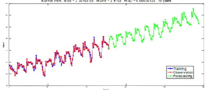
Figure 3. Forecast results of electricity consumption in Thailand by Squared Exponenti

Figure 4. Forecast results of electricity cons

Figure 1. Forecast results of electricity consumption in Thailand by Kernel Function Integration Techniques in Gaussian Proce

The experimental results were compared using four Kernel Function shown in Figure 4-7.

tricity consumption in Thailand by Rational Quadratic Kernel in Gaussian Processes

Forecast results of electricity consumption in Thailand by Squared Exponential Kernel in Gaussian Processes

Forecast results of electricity consumption in Thailand by Periodic Kernel in Gaussian Processes

Figure 1. Forecast results of electricity consumption in Thailand by Kernel Function Integration Techniques in Gaussian Processes

ic Kernel in Gaussian Processes

al Kernel in Gaussian Processes

During the session consisted of information unevenness. Can be simulated to periodic data. The function form is

( , ′) = exp ( (

′

)/

ℓ (31)

Functions for complex changes, but also slowly changing, created by Rational Quadratic Kernel. The function form is

( , ′) = ( (

′

) /

ℓ (32)

The function for linear longitudinal covariance with constant variance is constructed from Linear Kernel. The function form is

( , ′) = ( −ℓ)( ′−ℓ) (33)

Optimization by Composing Kernels

Bringing the four Kernel functions together into a new Kernel.

The Kernel functions are super-functional. (Superposition)

(Duvenaud, 2014) that makes each function independent of

each type with Sum and Product Structures.

+ = ( , ′)+ ( , ′) (34)

∗ = ( , ′)∗ ( , ′) (35)

Therefore, Kernel Squared Exponential (SE), Kernel Linear (LIN), and Time Kernel (PER), Rational Quadratic Kernel (RQ). All 4 Kernel functions come together as a new Kernel with the Sum and Product Structures. The new Kernel has the smallest tolerances in all 45 scenarios, namely the Kernel Function

∗ ∗ + ∗ +

APPLICATION: Forecasting Thailand electricity consumption with Kernel Function Integration Techniques in Gaussian Processes

Data set

Forecasting long term electricity consumption in Thailand with Kernel Function Integration Techniques in Gaussian Processes includes monthly electricity consumption data, gross domestic product (GDP) during January 2006 to December 2014. Data were from 108 months as training data and electricity consumption data of the next 24 months during January 2015 to December 2016 as data set for testing ability of algorithms that required only time variables (GDP was not required). This data set was called a test dataset. The historical dataset regarding these factors was collected annually from 2006 to 2016

Results of Forecasting

Forecasting results of electricity consumption in Thailand for the next 10 years by Gaussian Processes with combine Kernel Function Technique were shown in Figure2. The mean square error (MSE) and the mean absolute deviation (MAD) were equal to 7.4226E-11and6.2432E-06 and the mean absolute percentage error (MAPE) was equal to4.9192E-08.

Conclusion

The Kernel Functions of each type are governed by the Gaussian process effect of different time varying function models. For this research, a new Kernel function will be created based on time series data. The characteristics of the time series of a variable is composed of four parts: trends, cycles, variations from the session, and fluctuations from normal events. These 4 aspects consistent with each Kernel Function which is, the trend consist with the pattern of long-term trends and constant variability. It’s a feature of Kernel Squared Exponential and Linear Kernel. Cyclicality is

Figure 5. Forecast results of electricity consumption in Thailand by Linear Kernel in Gaussian Processes.

The errors from the above five Kernel function are compared in Table 1. The results showed that the error minimization capability of combine Kernel Function Technique model outperformed the other approaches.

Table 1. The comparison of errors from the five Kernel Function in Gaussian Processes

Kernel Function MSE MAPE MAD

Kernel Function Integration Techniques 7.9236E-11 5.9192E-08 7.2432E-06 Rational Quadratic Kernel 5.8722E-05 5.2095 0.0005841 Squared Exponential Kernel 2.651E-04 2.9692 0.0003668 Periodic Kernel 2.3616E-05 2.9768 0.0003613

Linear Kernel 18.3857 0.026335 3.2117

consistent with the function form for repeated but irregular data learning. It corresponds to the kernel of the quadratic algorithm, which is a function of complex change, but is slowly changing, and because of the fact that the time series data of one variable may consist of only two types. The selection of one Kernel Function may not cover the problem of forecasting.Taking the form of the four Kennel Functions together with the Sum and Product Structures, resulted in a new Kernel Function. The superposition make the variables that control the function of the independent functions of each category. The Kernel Function is at the center of the Gaussian process, because the predicted values are less error. The newly developed Kernel Functions can be applied to any problem or situation under all the time series data types, as viewed from the simulation results to compare the performance of the Kernel Function with the least deviation situation.

REFERENCES

Barkan, O., Weill, J., and Averbuch, A. 2016. Gaussian

process regression for out-of-sample extension. arXiv

preprint arXiv: 1603.02194.

Chea, J., and Wang, J. 2014. Short-term load forecasting using a kernel-based support vector regression combination

model. Applied Energy, 132, 602-609.

Claveria, O., Monte, E., and Torra, S. 2016. Modeling cross-dependencies between Spain’s regional tourism markets with an extension of the Gaussian process regression model. SERIEs, 1-17.

Duvenaud, D. 2014. Automatic model construction with

Gaussian processes (Doctoral dissertation, University of

Cambridge).

Duvenaud, D. K., Lloyd, J. R., Grosse, R. B., Tenenbaum, J. B., and Ghahramani, Z. 2013. Structure discovery in nonparametric regression through compositional kernel

search. In ICML (3) (pp. 1166-1174).

Ghoshal, S., and Roberts, S. 2016. Extracting predictive

information from Heterogeneous data streams using

Gaussian processes. arXiv preprint arXiv:1603.06202.

Hachino, T., Okubo, S., Takata, H., Fukushima, S., and

Igarashi, Y. 2015. Improvement of Gaussian process

predictor of electric power damage caused by Typhoons considering time-varying characteristics.

Kowal, D. R., Matteson, D. S., and Ruppert, D. 2016.

Gaussian processes for functional auto regression. ar Xiv

preprint arXiv:1603.02982.

Lei, Y., Guo, M., Cai, H., Hu, D., and Zhao, D. 2015. Prediction of Length-of-day Using Gaussian Process

Regression. Journal of Navigation, 68(03), 563-575.

Ludkovski, M., Risk, J., and Zail, H. 2016. Gaussian process

models for mortality rates and improvement factors.

Salcedo-Sanz, S., Casanova-Mateo, C., Munoz-Mari, J., and Camps-Valls, G. 2014. Prediction of daily global solar

irradiation using temporal Gaussian processes. Geoscience

and Remote Sensing Letters, IEEE, 11(11), 1936-1940.

Senanayake, R., O’Callaghan, S., and Ramos, F. (2016, March). Predicting spatio–temporal propagation of seasonal influenza using variational Gaussian process

regression. In Thirtieth AAAI Conference on Artificial

Intelligence.

Simionovici, A. M. 2016. Load prediction and balancing for

cloud-based voice-over-IP solutions (Doctoral dissertation,

University of Luxembourg, Luxembourg, Luxembourg). Sun, A. Y., Wang, D., and Xu, X. (2014). Monthly streamflow

forecasting using Gaussian process regression. Journal of

Hydrology, 511, 72-81.

Williams, C. K., and Rasmussen, C. E. 2006. Gaussian

processes for machine learning. The MIT Press, 2(3), 4.

Wilson, A., and Adams, R. (2013, February). Gaussian process

kernels for pattern discovery and extrapolation.

In International Conference on Machine Learning (pp.

1067-1075).

Wu, Q., Law, R., and Xu, X. 2012. A sparse Gaussian process regression model for tourism demand forecasting in Hong

Kong. Expert Systems with Applications, 39(5), 4769-4774.