AN ESTIMATION OF BLOCK NESTED
LOOP ALGORITHMS BASED ON JOIN
PROCESSING TIME
Rakesh Kumar Pandey, Dr. Deepak Arora, Deepak Shukla, Krishnakant Agrawal & Shashwat Shukla
[email protected] [email protected] [email protected] [email protected] [email protected]
Department of Computer Science and Engineering, Amity University, Lucknow, India
Abstract:
In databases, query processing is the mark able task under which join operation processing is the expensive operation that join two relations, occurring in the database system. In this paper the testing of the effectiveness of join algorithms has been proposed. In join operation between relations it is required to use those algorithms which take less time to process the join query efficiently in the database system. There are many algorithms are proposed previously for performing join operation. In this paper, a test has been proposed and based on the results of this test finding of the better algorithm among the join algorithm is presented by taking join processing time into consideration as the factor for comparing the join algorithms. It means that the analysis of the effective algorithm has been made based on the factor that which algorithms requires less time to join two relation. This test has been proposed by making block nested loop join algorithm to work on the tuples of the relations under join condition.
Keywords: Databases, Query Processing, Block Nested-Loop Join (BNLJ), and Join Processing Time.
1. Introduction
In the past different join algorithms had been introduced. These join algorithms required two or more relations to perform join between them based on the join condition provided. The differences between those join algorithms are proposed by comparing them on some factor like join processing time. The different factors on which comparison may be done are disk access time, rate of block transfer, seek time and join processing time. In this paper it has been proposed that based on the factor of join processing time the join algorithm are compared and the best one among them are reported or presented.
The buffer size plays an important role for calculating the costs of these join algorithms. The cost of join algorithms depends on the ways the buffer has been allocated during the process of joining relation. The join processing time for join algorithm are affected by the way the buffer has been allocated to the blocks of the relations that participated in the joining process. In this paper, it has been tested that which join algorithm process the join operation in less time between the targeted relations on some join condition.
In section 2 discussions has been made on the basis of the join algorithms previously developed and also analysis of effectiveness for the same is done as well. In section 3 the methodology, testing of join algorithms, reporting of test results, table and graphs has been proposed. In section 4 results of the testing of join algorithms based on the factor of join processing time has been presented and discussed as well. In section 5 concluding remarks and the future work have been discussed. In the final section references that support the proposed work has been presented.
2. Background
(2008)]. Some times it is necessary to work with multiple relations as they were contains data of same entity. Then a single SQL query can manipulate data from all the relations. Join are used to achieve this. Relations are joining on attributes that have the same data type and width in the relations [Bayross, (2008)].
There are many join algorithms for joining relations based on join condition. And, these algorithms scans the relations participated in the join operation to produce the joined relation as a result in the buffer of main memory. [Noh and Gadia, (2005a)]. Algorithms that support the proposed work for evaluating join are [Saheb, (2010)].
(1) Nested Loops Join (NLJ).
(2) Block Nested Loops Join (BNLJ –one block at a time) (3) Block Nested Loops Join (BNLJ –multiple block at a time)
Let us assume that, number of tuples in relation ‘r’=nr, number of tuples in relation ‘s’=ns, number of blocks of ‘r’=bR, number of blocks of relation ‘s’=bS, and number of blocks fits in main memory at once=Z. In Nested loop join algorithm, pairs of nested for loops are used to perform join operation. Relation ‘r’ is called outer relation and relation ‘s’ is the inner relation of the join, since the outer loop for relation ‘r’ contains the inner loop for relation ‘s’. The algorithm uses the notation tr.ts, where tr and ts are tuples; tr.ts denotes the tuples constructed by concatenating the attribute values of tuples tr and ts [Silberschatz et al., (2006a)].
In Nested Loop Join, it is very necessary to find out which relation is scanned by the outer loop and which is scanned by the inner loop of the join algorithm as the relations are stored in the form of file on the hard disk. The percentage of tuples in one relation of any database will be joined with tuples in the other relation of the same [Elmasri and Navathe, (2009)]. Algorithm for join applied on the block which resides on the main memory. This algorithm ensures that how the join performed in main memory. In the scanning of each tuple of ‘r’, it should be clear that the tuples of relation ‘s’ is scanned nr times, resulting nr*ns scanning for total tuples during join operation processing. In the scanning of one tuple for relation ‘r’, bS blocks of relation ‘s’ has been scanned. In the scanning of nr tuples for relation ‘r’, bS * nr scan needed. Total scans are equal to [nr * bS + bR]. nr seeks needed to scan ‘r’ and bR seeks needed to scan relation ‘s’ [Silberschatz et al., (2006b)]. Total seeks are equal to [nr + bR]. Complexity = O (nr*ns), where, nr and ns number of tuples contained in relation ‘r’ and ‘s’ respectively.
2.1.Block nested loop join (BNLJ-one block at a time)
In Block Nested Loop Join, when relations ‘r’ and ‘s’ has to be joined, the outer loop is for reading the blocks of relation ‘r’ and inner loop is reading the blocks of relation ‘s’. If relation ‘r’ and relation ‘s’ are small enough to fit into the main memory than the join operation is performed more effectively [Hagmann, (1986)].
In Block nested loop join, before performing the join operation the relations to be joined are first placed into the main memory [Noh and Gadia, (2005b)]. In Block Nested Loop Join algorithm, the number of disk accesses consists of two operations – one is to read the blocks of relation ‘r’ and other to access the disk for reading the blocks of relation ‘s’. [Dewitt et al., (1991)].
The Block Nested Loop Join algorithm is an advanced algorithm of the nested loop join algorithm which is used for transfer of blocks efficiently rather than transferring the tuples of the participating relations in the join operation. The block nested loop joins algorithm works by reading a block of tuples, from the outer and inner relation [Haris and Ramamohanarao, (1996)]. In BNLJ (one block at a time) chunks of each relation is transferred from hard disk to main memory where join operations is performed [Frey et al., (2009a)].
Algorithm: 2 Block Nested Loop Join (Block-at-a-time) [Frey et al., (2009b)] for each block bR of ‘r’ do
{ blocks of relation’r’ are scanned one by one. for each block bS of s do
{ blocks of relation’r’ are scanned one by one.
Compute bR bS in memory
}
}
2.2.Block Nested Loop Join (Z-2) (BNLJ-multiple block transfer)
Block Nested Loop Join (Multiple-Block-Transfer) divides memory into two parts. Zr blocks are used for relation ‘r’ and Zs blocks of main memory are used for relation‘s’ [Rupley, (2008)]. If (Z-2) blocks of relation ‘r’ are transferred to main memory and at (Z-1)th location in the main memory one block of relation ‘s’ is placed then the tuples of block of relation ‘s’ are compared with tuples in the (Z-2) blocks of relation ‘r’. After satisfying the join condition, join result is produced as a joined relation. In Block Nested Loop Join (Z-2), the number of blocks transferred for relation’r’ is (bR/ (Z-2)) and the number of blocks transferred for relation’s’ is ((bR/ (Z-2))*bS).
Algorithm: 3 Block Nested Loop Join (Z-2) [Silberschatz et al., (2006d)] for each block bR Z-2 of relation‘r’ do
{ //block from relation’s’
for each block bS of relation’s’ do { // tuples are scanned from bR for each tuple tr in bR do
{ //tuples are scanned from bS for each tuple ts in bS
{ Test pair (tr,ts) to see if they satisfy the join condition add tr.ts to the result
}
} } }
Block Nested Loop Join (Z-2) [Silberschatz et al., (2006e)]:-
Use the largest size that can fit in main memory, considering that space for the inner relation’s buffer and the output also. If memory has Z blocks, read Z-2 blocks of the outer relation at a time and also read a block of the inner relation to join it with all the Z-2 blocks of the outer relation.
Total Block transfer = [bR/Z-2]*bS+bR Total seeks = 2[bR/ (Z-2)] Complexity = O (n4)
2.3.Block nested loop join (z-3) [Shukla et al., (2011a)]
It has been assumed that total number of blocks that fits in the main memory is Z, total number of blocks in which relation ‘r’ fits on hard disk is bR, and total number of blocks in which relation ‘s’ fits on disk is bS. If Z-3 blocks of relation ‘r’ are transferred from disk to main memory and two blocks of relation ‘s’ are transferred from hard disk to main memory in one scan than the comparison is done and after satisfying the join condition the tuples are joined and transferred to output buffer at Zth location of main memory. Then, the total number of block transfers decreases as compared to when transfer of Z-2 blocks and one block of relation ‘r’ and relation ‘s’ has been done respectively. If bR is less than Z or bR equals to Z, then number of blocks transfers for relation ‘r’ is bR/ (Z-3), and number of blocks transfers for relation ’s’ is [(bR/ (Z-3))*bS]/2. Then, the total block transfers during ‘r’ join ‘s’ is the addition of number of block transfers from relation ‘r’ and number of block transfers from relation ‘s’ which is [(bR/(Z-3)) + [((bR/(Z-3))*bS)/2].
Let us assume that,
bR = total number of blocks on disk in which relation ‘r’ fits. bS = total number of blocks on disk which relation ‘s’ fits
xr = Points to first tuple of first block of relation ‘r’ that is transferred to main memory. xs = Points to first tuple (first) of first block of relation‘s’ in main memory.
bpr = Block Pointer i.e., it points to the block which is to be accessed.
bps = Block Pointer of blocks of relation‘s’ in main memory. i.e., it points to the block which is under consideration.
Z = Total number of blocks that can fit in main memory.
Algorithm: 4 Block Nested Loop Join (Z-3) [Shukla et al., (2011b)] i = bR / (Z-3)
j= [(bR/ (Z-3))*bS/2
While (i! =0) //blocks of relation ‘r’ outer loop { Move Z-3 blocks of relation ‘r’ in main memory. bpr points to first block of relation ‘r’ in main memory While (j! =0) //blocks of relation ‘r’ outer loop { Move two blocks of relation‘s’ at (Z-2) th and (Z-1) th location of main memory.
bps points to first block of relation‘s’ in main memory While (xr reaches end of block pointed by bpr)
{ Check whether all tuples of bpr are exhausted or not. While (xs reaches end of block pointed by bps) { Check whether bps are exhausted or not Compare tuples xr and xs and check the join condition, if it satisfies then adds xr.xs to output
buffer.
xs++;
} xr++;
} bps++; j- -; } bpr++; i- -;
}
3. Proposed Work
Join relations is on whole the frequently occurring operation in the database system. When block nested loop join algorithms are implemented and join operations are performed using these then it is interesting to look that how join processing time for joining two relation using two different algorithms changes dramatically. As the processing time for join operation varies depending upon the load on the system (load of processes) and the configuration as well. In support of the proposed work, the join processing time is measured in three ways when using block nested loop join (BNLJ-(Z-2)) and block nested loop join (BNLJ-(Z-3)) as the algorithms for joining relations :
Tuples in “Sled” > “Accounts” Tuples in “Sled” < “Accounts” Tuples in “Sled” = “Accounts”
Tuples in “Sled” > “Accounts”
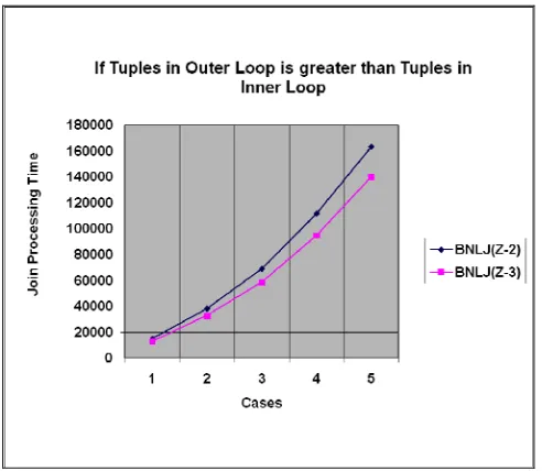
In the Table 1 there are two relations named “Sled” and “Accounts” are joined. It has been shown in the Table 1 that the number of tuples in the relation “Sled” is greater than the number of tuples in the relation “Accounts”. When joining of these two relations occurred and for the purpose of testing the number of tuples in relation “Sled” is incremented by 500 tuples and the number of tuples in relation “Accounts” is incremented by 50 tuples in each case then joining is performed by using two algorithm named block nested loop join (BNLJ-(Z-2)) and block nested loop join (BNLJ-(Z-3)) and join processing time taken by both the algorithms is recorded.
It has been analyzed from the first entry in Table 1 that when number of tuples in relation “Sled” is 1000 and the number of tuples in relation “Accounts” is 75 then the recorded join processing time when using block nested loop join (Z-3) is 13,013 ms which is less than that of 15015 ms recorded by using block nested loop join (Z-2) for joining these two relations. It has been analyzed from the other entries that the recorded join processing time when using block nested loop join (Z-3) is less than that of recorded join processing time when using block nested loop join (Z-2) for joining these two relation in every case. So, on the whole the block nested loop join (Z-3) is better than block nested loop join (Z-2) algorithm when join processing time is the comparing factor.
When the graph in fig.1 has been analyzed, it shows that there are two lines one shows the processing time taken by using block nested loop join (Z-2) algorithm and other shows the processing time when using block nested loop join (Z-3) algorithm for joining the relation “Sled” that have greater number of tuples with the relation “Accounts” under test.
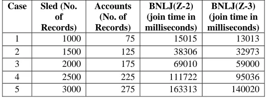
Table 1. Tuples in relations “sled” > “accounts” with join processing time in milli-seconds.
Case Sled (No. of Records)
Accounts (No. of Records)
BNLJ(Z-2) (join time in milliseconds)
BNLJ(Z-3) (join time in milliseconds)
1 1000 75 15015 13013 2 1500 125 38306 32973 3 2000 175 69010 59000
4 2500 225 111722 95036
5 3000 275 163313 140020
The y-axis shows, the join processing time. When the tuples in “Sled” as relation at outer loop is greater than the number of tuples in “Accounts” as relation at inner loop, the time taken by block nested loop join (Z-3) algorithm to join these two relations is always less than the time taken when using block nested loop join (Z-2) algorithm for the same. So, by the analysis of the result recorded by the test performed it has been concluded that block nested loop join (Z-3) algorithm gives better results than block nested loop join (Z-2) algorithm for joining two relations “Sled” and “Accounts”, when join processing time is the comparison factor between these two algorithms.
Fig 2 Graph showing join processing time for BNLJ (Z-2) and BNLJ (Z-3), when tuples in “Sled” is less than tuples in relation “Accounts” based on
Tuples in “Sled” < “Accounts”
In the Table 2 there are two relations named “Sled” and “Accounts” are joined. It has been shown in the Table 2 that the number of tuples in the relation “Sled” is less than the number of tuples in the relation “Accounts”. When joining of these two relations occurred and for the purpose of testing the number of tuples in relation “Sled” is incremented by 50 tuples and the number of tuples in relation “Accounts” is incremented by 500 tuples in each case then joining is performed by using two algorithm named block nested loop join (Z-2) and block nested loop join (Z-3) and join processing time taken by both the algorithms is recorded.
It has been analyzed from the first entry in Table 2 that when number of tuples in relation “Sled” is 75 and the number of tuples in relation “Accounts” is 1000 then the recorded join processing time when using block nested loop join (Z-3) is 14,014 ms which is less than that of 17,017 ms recorded by using block nested loop join (Z-2) for joining these two relations. It has been analyzed from the other entries that the recorded join processing time when using block nested loop join (Z-3) is less than that of recorded join processing time when using block nested loop join (Z-2) for joining these two relations in every case. So, on the whole the block nested loop join (Z-3) is better than block nested loop join (Z-2) algorithm when join processing time is the comparing factor.
When the graph in fig.2 has been analyzed, it shows that there are two lines, one shows the processing time taken by using block nested loop join (Z-2) algorithm and other shows the processing time when using block nested loop join (Z-3) algorithm for joining the relation “Sled” that have less number of tuples with the relation “Accounts” under test. The y-axis shows, the join processing time. When the tuples in “Sled” as relation at outer loop is less than the number of tuples in “Accounts” as relation at inner loop, the time taken by block nested loop join (Z-3) algorithm to join these two relations is always less than the time taken when using block nested loop join (Z-2) algorithm for the same. So, by the analysis of the result recorded by the test performed it has been concluded that block nested loop join (Z-3) algorithm gives better results than block nested loop join (Z-2) algorithm for joining two relations “Sled” and “Accounts”, when join processing time is the comparison factor between these two algorithms.
Table 2. Tuples in relations “sled” < “accounts” with join processing time in milli-seconds.
Case Sled (No. of Records)
Accounts (No. of Records)
BNLJ(Z-2) (join time in milliseconds)
BNLJ(Z-3) (join time in milliseconds)
1 75 1000 17017 14014
2 125 1500 42983 37037
3 175 2000 81290 71011
4 225 2500 129006 112323
5 275 3000 190010 164985
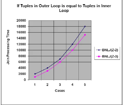
Fig 3 Graph showing join processing time for BNLJ (Z-2) and BNLJ (Z-3) when tuples in “Sled” is equal to tuples in relation “Accounts” based on
Tuples in “Sled” = “Accounts”
In the Table 3 there are two relations named “Sled” and “Accounts” are joined. It has been shown in the Table 3 that the number of tuples in the relation “Sled” is equal to the number of tuples in the relation “Accounts”. When joining of these two relations occurred and for the purpose of testing the number of tuples in relation “Sled” is incremented by 50 tuples and the number of tuples in relation “Accounts” is incremented by 50 tuples in each case then joining is performed by using two algorithm named block nested loop join (Z-2) and block nested loop join (Z-3) and join processing time taken by both the algorithms is recorded.
It has been analyzed from the first entry in Table 3 that when number of tuples in relation “Sled” is 75 and the number of tuples in relation “Accounts” is 75 then the recorded join processing time when using block nested loop join (Z-3) is 1,001 ms which is less than that of 2,002 ms recorded by using block nested loop join (Z-2) for joining these two relations. It has been analyzed from the other entries that the recorded join processing time when using block nested loop join (Z-3) is less than that of recorded join processing time when using block nested loop join (Z-2) for joining these two relations in every case. So, on the whole the block nested loop join (Z-3) is better than block nested loop join (Z-2) algorithm when join processing time is the comparing factor.
When the graph in fig.3 has been analyzed, it shows that there are two lines one shows the processing time taken by using block nested loop join (Z-2) algorithm and other shows the processing time when using block nested loop join (Z-3) algorithm for joining the relation “Sled” that have equal number of tuples with the relation “Accounts” under test.
Table 3. Tuples in relations “sled” = “accounts” with join processing time in milli-seconds.
Case Sled (No. of Records)
Accounts (No. of Records)
BNLJ(Z-2) (join time in milliseconds)
BNLJ(Z-3) (join time in milliseconds)
1 75 75 2002 1001
2 125 125 4003 3003
3 175 175 7007 6006
4 225 225 12012 10010 5 275 275 18018 15173
The y-axis shows, the join processing time. When the tuples in “Sled” as relation at outer loop is equal to the number of tuples in “Accounts” as relation at inner loop, the time taken by block nested loop join (Z-3) algorithm to join these two relations is always less than the time taken when using block nested loop join (Z-2) algorithm for the same. So, by the analysis of the result recorded by the test performed it has been concluded that block nested loop join (Z-3) algorithm gives better results than block nested loop join (Z-2) algorithm for joining two relations “Sled” and “Accounts”, when join processing time is the comparison factor between these two algorithms.
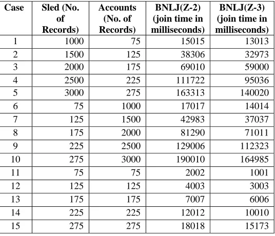
4. Result And Discussion
When two relations are joined it takes time to process join operation that depends on the join algorithm being used at the time of joining the relations like block nested loop (Z-2) and block nested loop (Z-3) algorithm. If “Sled” is the relation at the outer loop and the relation “Accounts” at the inner loop of the join algorithm than their exists three ways based on which join processing time has been calculated and tests are performed to analyze and find out the better join algorithm among the two block nested loop 2) and block nested loop (Z-3), these are: tuples in “Sled” > “Accounts”, tuples in “Sled” < “Accounts”, and tuples in “Sled” = “Accounts”.
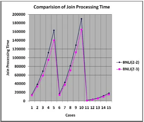
Table 4. Comparison of Join Processing Time (in milli-seconds).
Case Sled (No. of Records)
Accounts (No. of Records)
BNLJ(Z-2) (join time in milliseconds)
BNLJ(Z-3) (join time in milliseconds)
1 1000 75 15015 13013
2 1500 125 38306 32973
3 2000 175 69010 59000
4 2500 225 111722 95036
5 3000 275 163313 140020
6 75 1000 17017 14014
7 125 1500 42983 37037
8 175 2000 81290 71011
9 225 2500 129006 112323
10 275 3000 190010 164985
11 75 75 2002 1001
12 125 125 4003 3003
13 175 175 7007 6006
14 225 225 12012 10010
15 275 275 18018 15173
If the number tuples in the relation “Sled” is greater than the number of tuples in the relation “Accounts”, it has been analyzed by the testing of the join algorithms named block nested loop 2) and block nested loop (Z-3), that when these two are used for joining the relation “Sled” with the relation “Accounts” the join processing time taken by block nested loop (Z-3) algorithm is less than that of the join processing time taken by block nested loop (Z-2) algorithm.
When the number of tuples in the relation “Sled” is less than the number of tuples in the relation “Accounts” and again “Sled” is the relation at outer loop and “Accounts” is the relation at inner loop of the join algorithms block nested loop (Z-2) and block nested loop (Z-3. It has been proved that, the block nested loop (Z-3) algorithm gives better results than block nested loop (Z-2) algorithm, when join processing time is the comparison factor between these two algorithms. It has been analyzed that when the number of tuples in the relation “Sled” is equal to the number of tuples in the relation “Accounts” and again “Sled” is the relation at outer loop and “Accounts” is the relation at inner loop of the join algorithms block nested loop (Z-2) and block nested loop (Z-3) then the block nested loop (Z-3) algorithm gives better results than block nested loop (Z-2) algorithm, when join processing time is the comparison factor between these two algorithms.
5. Concluding Remarks and Future Work
Acknowledgement
The authors are very thankful to their respected Mr. Aseem Chauhan, Chairman, Amity University, Lucknow, Maj. Gen. K.K. Ohri, AVSM (Retd.), Director General, Amity University, Lucknow, India, for providing excellent computation facilities in the University campus. Authors also pay their regards to Prof. S.T.H. Abidi, Director and Brig. U.K. Chopra, Deputy Director, Amity School of Engineering, Amity University, Lucknow for giving their moral support and help to carry out this research work.
Reference
[1] Deepak Shukla, Rakesh Kumar Pandey, Deepak Arora and Ajai Kumar Yadav (9-10th April 2011): An effective approach for join operation processing. 2nd National conference on Global Trends and Innovations in Computer Application and Informatics, India. [2] Noh, S.Y. and S.K. Gadia (2008): Benchmarking temporal database models with interval based and temporal element-based
time-stamping. Journal of System software, 81:1931-1943.
[3] Robert B. Hagmann (1986): An Observation on Database Buffering Performance Metrices. Proceedings of the 12th International conference on very large Databases, Kyoto.
[4] M. H. Saheb. (2010): Efficient Algorithm for overlap – join , Information Technology Journal, 10:201206.
[5] David J. Dewitt, Jeffrey. F. Naughton and Donovan A. Schneider. September (1991): An Evaluation of Non-Equijoin Algorithms, Proceedings of the 17th International Conference on Very Large Databases, Barcelona.
[6] Philip W. Frey, Romulo Gonalves, Martin Kersten and Jens Teubner (2009): Cyclo Join: A Join that Spins without Getting Dizzy. In the proceedings of ACM.
[7] Evan P. Haris and Kotagiri Ramamohanarao (1996): Join Algorithm Costs Revisited Technical Report 93/5.
[8] Laura M. Haas, Michael J. Carey and Miron Livny. May (1993): SEEKing the Truth about Ad Hoc Join Costs , Technical Report #1148.
[9] Seo-young Noh and Shashi K. Gadia ( 2005): Efficient Self Join Algorithm in Interval-based Temporal Data Models. Technical Report, Department of Computer Science, Iowa State University, Ames, Iowa, USA. Http://archives.cs.iastate.edu/documents/disk0/00/00/03/86/index.html.
[10] Michael L. Rupley, Jr. (2008): Introduction to Query Processing and Optimization. http://www.cs.iusb.edu/technical_repots/TR- 20080105-1.pdf
[11] Abraham Silberschatz, Henry F. Korth and S. Sudarshan. (2006): Database System Concepts, 5th Edition, Mc Graw Hill Higher Education [ISBN: 007-124476-X].
[12] Elmasri. R. and S.B. Navathe. (2009): Fundamentals of Database Systems. 5th Edition, Pearson Education. [ISBN: 978-81-317-1625-0].