www.nat-hazards-earth-syst-sci.net/9/135/2009/ © Author(s) 2009. This work is distributed under the Creative Commons Attribution 3.0 License.
and Earth
System Sciences
Rainfall thresholds and flood warning: an operative case study
V. Montesarchio, F. Lombardo, and F. Napolitano
Department of Hydraulics, Highways and Roads, “Sapienza” University of Rome, 00184 Rome, Italy
Received: 4 April 2008 – Revised: 8 January 2009 – Accepted: 19 January 2009 – Published: 16 February 2009
Abstract. An operative methodology for rainfall thresholds definition is illustrated, in order to provide at critical river section optimal flood warnings. Threshold overcoming could produce a critical situation in river sites exposed to alluvial risk and trigger the prevention and emergency system alert. The procedure for the definition of critical rainfall thresh-old values is based both on the quantitative precipitation ob-served and the hydrological response of the basin. Thresh-olds values specify the precipitation amount for a given dura-tion that generates a critical discharge in a given cross secdura-tion and are estimated by hydrological modelling for several sce-narios (e.g.: modifying the soil moisture conditions). Some preliminary results, in terms of reliability analysis (presence of false alarms and missed alarms, evaluated using indica-tors like hit rate and false alarm rate) for the case study of Mignone River are presented.
1 Introduction
Floods analysis aims to face residual risk, due to failure of technical systems, or due to the rare flood which exceeds the design flood. Forecasting catastrophic events with ad-vance allows civil protection measures to restrain the socio-economic impact.
Naturally, the flood forecasting methods are different in relation to the basins size and time of concentration (Rosso, 2002). If a 12 h advance warning is needed, necessarily the forecasting methods are based on different parameters. For large basins (>10 000 km2) the concentration time is higher then 10 h and the flood forecast warning in one section can be made on the basis of the water levels recorded in upstream sections. For intermediate basins (400–10 000 km2) the
con-Correspondence to: V. Montesarchio
centration time varies between 3 and 10 h and the flood fore-casting can be made mainly on the basis of precipitation mea-surements, eventually integrated with forecasted precipita-tion. For small basins (<400 km2), the concentration time is smaller than 3 h, and the flood forecasting warning can be made only on the basis of precipitation forecasts.
Warning methods work in the precipitation domain and provide rainfall thresholds (in terms of rainfall rate, duration and space extent) for river system critical state. Threshold overcoming could produce a critical situation in river sites exposed to alluvial risk and trigger the prevention and emer-gency system alert (Georgakakos, 1995).
In this work the critical rainfall thresholds for Mignone River cross section are defined to set a warning for critical flood events. This paper is developed as follows: firstly, an overview of the methodology for rainfall thresholds estima-tion is given. Secondly, the methodology is applied to the case study of Mignone River. Finally, rainfall thresholds re-liability is evaluated and results are discussed.
2 Flood rainfall thresholds
Generally, rainfall thresholds identify precipitation critical values, that could be used both in the context of landslides and debris flow hazard forecasting (Neary et al., 1987; An-nunziati et al., 1996; Crosta and Frattini, 2000) and in the flood forecasting or warning (Carpenter et al., 1999; Mancini et al., 2002; Georgakakos, 2006; Martina et al., 2006).
In the flood warning context, when critical values are over-came, effects of flooding are expected. Rainfall thresholds specify the precipitation amount for a given duration that generates a critical discharge in a given cross section. 2.1 Critical cross section identification
hydraulic geometry, critical water stage is known and critical discharge is estimated by the stage-discharge curve (Rosso, 2002).
When the basin is ungauged, neither hydraulic geometry or hydraulic data are known, so is more difficult to establish which is the critical cross section and relative discharge. For choosing the critical cross section, the first element is how-ever the historical one, with information about past floods events. This knowledge allows to identify hydraulic risks ar-eas. If there are no past events recorded, it does not mean that in the future flood events will not occur. It is also possible that in the past flood events occurred, but there is no informa-tion available. A way to identify hydraulic risks secinforma-tion is to refer to hydraulic risks planning (i.e. in Italy “Piani di Assetto Idrogeologico” or “Piani Stralcio di Assetto Idrogeologico”, in which possible flooding areas are identified), often based on a methodology that allows to identify both critical cross sections and critical discharge (or hydraulic stage), the hy-draulic simulation. It requires, however, to know some cross sections of the river, to perform at least one-dimensional flow propagation.
However, in case of no available information, the most critical section could be identified as the outlet of the basin, as all the upstream contributions flow in this section, arriving from the entire drainage area.
Assuming that the critical cross section was identified, the next step is to evaluate the critical discharge. As it has been told, it is more difficult when stream flow data (or stage data and stage-discharge curve) are not available, and the hy-draulic modelling is not possible. A feasible solution is to use regional method to evaluate the critical discharge. For example, the flood index method (Dalrymple, 1960) could be used. This method, based on the statistical regionaliza-tion, allows to replace the time with the space and to use the set of hydrometric observations of a homogeneous area to fit the lack of discharge data in the critical cross sections.
Given a return periodT relative to the critical cross sec-tions, the peak discharge is expressed as the product of two terms: the scale factor of the examined site (the index flood) and the dimensionless growth factor, which has regional va-lidity. Naturally, the index flood of the site and the growth factor of the homogeneous region need to be estimated. In gauged sections it is clearly possible to estimate the index flood directly, by calculating the arithmetic mean of the avail-able observations, in ungauged sections indirect methods have to be used (Brath et al., 2001). Using this approach, the rainfall thresholds is not referred to a critical discharge value, but to different return periods discharge (i.e. 2, 5, 10, 20, 50, 100 years).
2.2 Simulation model
The methodology is based on the hydrological simulation: the river basin closed at the critical cross section is outlined with a rainfall/runoff model, opportunely calibrated. The
in-verse hydrologic problem is iterative solved to identify, for given durationd, the cumulative rainfall correspondent to the critical discharge.
When the basin is ungauged, the calibration is more dif-ficult, because of the lack of observed data. The litera-ture however contains numerous studies on the possibly ap-proaches. First of all, it can be used a model including only physically based parameter that can be measured, with no calibration procedures. A second possibility is to extrapolate the parameters of the ungauged sites from those of gauged sites, using regression analysis: in this case could be dif-ficult to relate all model parameters with proper catchment characteristics (Nathan and McMahon, 1990; Servat and Dezetter, 1993; Sefton and Boorman, 1997). Then, there is the possibility of relating the response of the catchment to its morphologic or topologic aspects, using a geomorphologic approach: geomorphologic IUH (GIUH) (Rodriguez-Iturbe and Valdes, 1979) or width function based IUH (WFIUH) (Kirkby, 1976; Mesa and Mifflin, 1986; Naden, 1992). Fi-nally, calibration is possible using synthetic flow duration curves generated for ungauged sites based on regional anal-ysis methods (Yu and Yang, 2000). Thus the methodology could be applied also at ungauged sites, in a more general framework of regional analysis methods, with a grater ef-fort in the model calibration phase, not based on observed data but on opportunely obtained synthetic values. Once the model is calibrated, the inverse hydrologic problem is solved for different return period discharge (cfr. Sect. 2.1).
In this study a semi-distributed rainfall/runoff model is chosen, to consider spatial variability of physical processes. In fact, even if the threshold will be expressed in terms of cumulative precipitation, it seems important to evaluate the variability of response with spatial variability of input, be-cause critical situation could be triggered by local phenom-ena, and a semi-distributed model allows to highlight these effects.
2.3 Rainfall thresholds evaluation
The critical reference discharge could be reached and over-came for different space-time configurations of rain fields. One possible simplified solution is to evaluate globally the cumulative precipitation (P) over the basin, after a time (d) from the beginning of the thunderstorm. Rainfall thresholds are generally function of the critical cross section character-istics, but also of the boundary conditions and the rain event type, especially:
– soil imbibition condition at the beginning of thunder-storm;
– temporal evolution of precipitation.
PAST EVENTS
YES
NO
HYDRAULIC GEOMETRY
Model Calibration on data
FLOOD RAINFALL TRESHOLDS EVALUATION
Lack of informations No past events
YES
Critical stage
CRITICAL DISCHARGE
Stage-discharge curve
INVERSE HYDROLOGICAL PROBLEM
NO
Regional analysis Flood index methods
RAINFALL-RUNOFF MODEL
Model Calibration (regional approach based on synthetic flow duration curves) Physically based model (no calibration)
Geomorphological model (WFIUH) Qc
CRITICAL DISCHARGE
QT (T=2,5,10,20,50,100 yrs)
RAINFALL-RUNOFF MODEL
Fig. 1. Flood rainfall thresholds evaluation.
Mignone SS n. 1 Aurelia
0.0 1.0 2.0 3.0 4.0 5.0 6.0 7.0 8.0 9.0 10.0
0 10 20 30 40 50 60 70 80
Progressive
ms
lm Hmax=3.80 m
Fig. 2. Critical section hydraulic configuration.
Figure 1 illustrated the steps of rainfall thresholds evalua-tion procedure.
3 The case study: Mignone River
3.1 Basin characteristics
The Mignone River begins on the Sabatini Mounts (633 m.s.l. m) and flows into the Tirreno Sea. The river to-tal length is 62 km. The basin surface is about 560 km2, the average elevation is 233 m a.s.l. The hydraulic behaviour is very variable, typical of a torrential regimen.
Table 1. Initial conditions: API5 (SCS, 1986).
AMC Class 5-days antecedent rainfall API5(mm) dormant season growing season I dry <12.7 <35.5 II average 12.7÷28.0 35.5÷53.3 III saturated >28.0 >53.3
Table 2. Rain gauges events AMC (SCS, 1986) classification.
AMCI AMCII AMCIII
16 5 7
The soil is constituted by the 25% of vulcanites, in cor-rispondence of the reliefs. Coming down towards valley are present sand and conglomerates (14%), clays (9%), antropiti (2%), but above all Flysch (41%) and alluvial deposits along the river (9%).
3.2 Mignone River: data sets
3.2.1 Critical cross section identification
In this work the critical hydraulic cross section is identi-fied by a preliminary historical-documentary analysis of past flood events.
From the information available on Sistema Informativo Catastrofi Idrogeologiche (SICI) of CNR-GNDCI website it was found that in the last century Mignone River over-flowed 3 times (08/11/1934, 27/12/1959, 16/11/1962) in Tar-quinia area along the S.S. Aurelia. In first approximation, it has been considered the overflowed fluvial cross sections coinciding with the monitored cross sections “S.S. Aurelia” (drainage area 440 km2), therefore identified as critical cross section. Given cross section geometry (Fig. 2) and stage-discharge curve used by authorities, the critical reference dis-charge, Qc was identified to be equal to 131.0 m3/s.
3.2.2 Hydrometric and pluviometric data
Table 3. Flood events in Mignone River Basins.
date Qp(m3/s)
15–20/04/1999 135.41 14–17/12/1999 69.57 31/03–02/04/2000 103.06 09–13/04/2000 422.09 28/01–01/02/2001 207.36 11–14/12/2002 160.33 05–08/01/2003 179.38 26–29/11/2003 235.17 04–08/05/2004 101.04 04–07/12/2004 498.03 25–31/12/2004 530.89 18–21/01/2005 88.24 02–06/03/2005 367.75 08–11/09/2005 63.96 05–07/11/2005 233.21 25–28/11/2005 333.66 02–05/12/2005 217.43 05–07/12/2005 210.72 08–11/12/2005 260.18 01–04/01/2006 68.18 19–24/02/2006 518.54 05–08/03/2006 399.52 15–18/03/2006 490.69 16–19/09/2006 110.81 20–23/10/2006 78.55 08–10/12/2006 171.69 08–11/02/2007 144.98 24–27/03/2007 248.63
Mignone River Basin from 1999 to 2007, for which pluvio-metric data are available.
3.2.3 Radar data
The Polar 55C is located 15 km south-east of Rome, in the Tor Vergata research area (lat. 41◦5002400N, lon. 12◦3805000E, 102 m above sea level). Polar 55C is a C-band (5.5 GHz,λ=5.4 cm). Doppler weather radar with po-larization ability and with a 0.9◦beamwidth. The radar has the capability to transmit and receive horizontally and verti-cally polarized signals on alternate pulses, allowing not only the measurement of the widely used horizontally reflectivity factor (Zh), but also the differential reflectivity (Zdr) and the differential phase shift (8dp). Radar measurements are
ob-tained by averaging 64 pulses with a range-bin resolution of 75 m, covering an area with a radius up to 120 km from the radar site. The temporal resolution is five minutes.
To remove spurious returns from the data, a polarimetry-based ground clutter removal algorithm was applied (Lom-bardo et al., 2006).
Fig. 3. Study area and radar position.
Table 4. Radar events AMC (SCS, 1986) classification.
AMCI AMCII AMCIII
6 3 2
In order to convert the radar data into rainfall rates, was used an algorithm based on a Z-R relation. For C-band by means of a non-linear regression analysis, the following Z-R relation was obtained (Russo et al., 2005):
R=7.27×10⁻²Zh0.62 (1)
where Zh is the reflectivity factor [mm6·mm−3] and R is rainfall intensity [mm·h−1].
After a transformation from Polar to Cartesian coordi-nates, a regular grid (2 km×2 km) over the basin was built (Fig. 3). From each time interval rain intensity values for each pixel were obtained intensity and then total cumulative rainfall Radar rainfall temporal resolution is 30 min.
Radar measurements are classified in AMC classes in Ta-ble 4. It is to be underlined that the radar data not coincide with the floods events summarized in Table 3. In fact, as it is shown in Table 5, only the November 2003 events is covered by both radar and raingauges. Other radar measure-ments were taken in not flood periods.
3.3 Simulation model
Table 5. Radar measurement intervals.
Measurement interval Qp(m3/s)
22/10/2003 6.25.34 23/10/2003 7.31.34 0.25 26/11/2003 6.56.02 27/11/2003 18.46.46 235.17 26/02/2004 10.35.53 27/02/2004 7.00.53 30.01 01/03/2004 8.08.04 01/03/2004 15.20.53 55.43 11/03/2004 8.50.57 11/03/2004 16.40.54 14.73 24/03/2004 12.57.59 25/03/2004 14.30.34 7.16 07/05/2004 8.07.59 07/05/2004 16.36.34 37.69 12/05/2004 5.42.59 12/05/2004 16.41.35 5.71 14/05/2004 8.16.34 14/05/2004 18.16.35 3.28 05/08/2004 8.55.55 05/08/2004 17.31.35 0.09
The basin area was subdivided in two subbasins (Fig. 4): the first closed to Rota and the second closed to the critical cross section; for both subbasins, for rainfall/runoff transfor-mation was used the modified Clark model (Kull and Feld-man, 1998; Peters and Easton, 1996), that allows using a semi-distributed approach and considering explicitly physi-cal processes space variability. For hydrologiphysi-cal losses was used a gridded SCS-CN model (SCS, 1971, 1986), while for flood wave propagation was used the Lag model (Pilgrim and Cordery, 1993).
The Meteorologic model was a gridded precipitation, dis-tributed from rain gauges data with isohyetes method every 30 min.
The hydrologic model calibration and verification are per-formed for the following flood events:
– AMCI class: calibration event 05/11/2005, control event 10/12/2006;
– AMCII class: calibration events 22/02/2006, 30/01/2001, control event 25/03/2007; – AMCIII class: calibration events 04/12/2005,
06/12/2005, control event 10/12/2005.
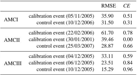
In Fig. 5 calibration and validation of hydrologic model for AMCIII class are shown. To evaluate model performance, two indicators were considered (Table 6).
The Root Mean Squared Error (RMSE, Eq. 1) mea-sures the overall agreement between observed and modelled events. It has non-negative value and no upper bound. If the model were perfect, RMSE would be zero.
RMSE=
v u u u t
n P
i=1
Qi− ˆQi
2
n (2)
In Eq. (1), Qi and Qˆi are the observed and the modelled
values at timei, withntotal number of time intervals. Gen-erally, for high flows this index can provide good measure of model performance (Karunanithi et al., 1994)
Fig. 4. Mignone model in HMS.
Table 6. Hydrological model performance.
RMSE CE
AMCI calibration event (05/11/2005) 35.90 0.51 control event (10/12/2006) 31.50 0.31
AMCII
calibration event (22/02/2006) 61.70 0.78 calibration event (30/01/2001) 39.46 0.00 control event (25/03/2007) 28.87 0.66
AMCIII
calibration event (04/12/2005) 33.11 0.59 calibration event (06/12/2005) 23.51 0.84 control event (10/12/2005) 15.29 0.96
The other indicator used is the Coefficient of Efficiency (CE; Nash and Sutcliff, 1970, Eq. 2), that is proportional to variance of observed data. CE can range between minus in-finity and one, which represents a perfect model. If CE is zero, there is no difference between using the mean of ob-served data or simulated values. If CE is negative, the mean of observed data is better then the model.
CE=1−
n P
i=1
Qi− ˆQi
n P
i=1
Qi−Q
(3)
In Eq. (1), Qi and Qiˆ are the observed and the modelled
values at timei, withntotal number of time intervals, andQ
is the mean of observed data.
S.S. Aurelia Calibration
0.0 50.0 100.0 150.0 200.0 250.0 300.0
05/12/2005 10.30 06/12/2005 10.30 07/12/2005 10.30
date
Q(
m
3/s
)
0.0
2.0
4.0
6.0
8.0
10.0
12.0
h(
m
m
)
Qobserved Qsimulated
S.S. Aurelia Validation
0.0 50.0 100.0 150.0 200.0 250.0 300.0
08/12/2005 15.30 09/12/2005 15.30 10/12/2005 15.30
date
Q(
m
3/s
)
0.0
2.0
4.0
6.0
8.0
10.0
12.0
h
(mm)
Qobserved Qsimulated
Fig. 5. Calibration and control of class AMC III hydrologic model for the Mignone River basin on the base of the observed hydrographs at
“S.S. Aurelia” gauge station in December 2005.
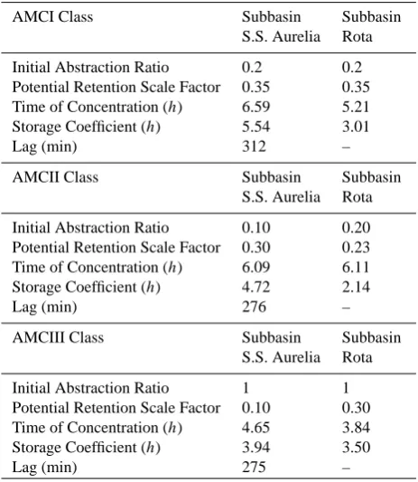
Table 7. Hydrologic parameters values.
AMCI Class Subbasin Subbasin S.S. Aurelia Rota Initial Abstraction Ratio 0.2 0.2 Potential Retention Scale Factor 0.35 0.35 Time of Concentration (h) 6.59 5.21 Storage Coefficient (h) 5.54 3.01
Lag (min) 312 –
AMCII Class Subbasin Subbasin S.S. Aurelia Rota Initial Abstraction Ratio 0.10 0.20 Potential Retention Scale Factor 0.30 0.23 Time of Concentration (h) 6.09 6.11 Storage Coefficient (h) 4.72 2.14
Lag (min) 276 –
AMCIII Class Subbasin Subbasin S.S. Aurelia Rota Initial Abstraction Ratio 1 1 Potential Retention Scale Factor 0.10 0.30 Time of Concentration (h) 4.65 3.84 Storage Coefficient (h) 3.94 3.50
Lag (min) 275 –
condition model there is the worst performance, mainly for the low CE values.
In Table 7 are summarized all the numerical values of the model parameters.
3.4 Rainfall thresholds evaluation
The inverse hydrologic problem was solved to identify the rainfall fields configuration that implies the critical discharge value overcoming. Several scenarios were simulated, analyz-ing basin response to 4 hyetotypes (Rosso, 2002):
Hyeto_1
15 20 25 30 35
3 6 9 12 15 18 21 24
d(h)
AMCI AMCII AMCIII
AMCII
15.0 20.0 25.0 30.0 35.0
3 6 9 12 15 18 21 24
d(h)
h
cum
(mm)
hyeto_1 hyeto_3
hyeto_2 hyeto_4
Fig. 6. Rainfall thresholds for different hyetotype, fixing class AMC
II, and for different AMC classes for the step hyetograph (Hyeto 1). In ordinate the cumulative rainfall amount (in millimeter), in abscissa the duration (in hours).
– step hyetograph (Hyeto 1);
– triangular increasing rate hyetograph (Hyeto 2); – triangular decreasing rate hyetograph (Hyeto 3); – isosceles triangular hyetograph (Hyeto 4).
Event-Hyetotypes
0 10 20 30 40 50 60 70 80 90 100
0 10 20 30 40 50 60 70 80 90 100
d/dtot (% )
hcu
m
/hcu
m
to
t
(%
)
Observation 10/12/2005 Hyeto_1
Hyeto_2
Hyeto_3
Hyeto_4
Fig. 7. Association to hyetotype: in ordinate % cumulative rainfall,
in abscissa % duration. Event 10/12/2005.
4 Preliminary results: reliability evaluation
In this work the reliable thresholds were tested following these steps:
– identification of significative durationd∗ and associa-tion of observed pluviometric events with a standard hyetotype;
– reliability evaluation in terms of right, false and missed alarms.
Preliminary it was necessary to establish some criteria for de-termining the beginning of actual runoff (d∗, from when cu-mulative rainfall amounts were calculated) and for dividing precipitation events. Two parameters have been fixed (Rosso, 2002):
– significant rain: value of cumulative rainfall, discrimi-nating between state of rain and of not-rain, identified with initial infiltration of the loss model;
– system relaxation time: time of concentration of the river basin closed to the critical cross section.
To identify the reference hyetotype, given the irregularity of real hyetographs, a “likelihood” approach is used. The hyeto-type was estimated considering a differences minimization. An example is shown in Fig. 7, for the event observed on 10/12/2005.
To estimate the rain thresholds reliability is necessary to investigate on the presence of any missed alarms or false alarms. It is defined:
– missing alarm (MA): the flood event exceeds the criti-cal reference discharge in the criticriti-cal cross section, but the recorded precipitation does not exceed the rainfall threshold.
– false alarm (FA): the rainfall threshold is overcame, but the observed discharge is lower than critical reference discharge.
Table 8. Two-by-two contingency table.
Forecasts
Observations Warning W No Warning W0 Total
Event E h m e
Non Event E0 f c e0
Total w w0 n
Obviously presence of FA and above all of MA invalidate rainfall thresholds reliability as warning tool. A possible way to assess the performance of the proposed method is using a two-by-two contingence table, as illustrated in Table 8. The table is structured as follows: thenobservations are divided in Event E (critical discharge overcame) and Non Event E (critical discharge not overcame). If an event occurred and a warning was issued the outcome is an hit (withhthe total number of hits); if an event did not occur but a warning was issued the outcome is a false alarm, (withf the total number of false alarms); if an event occurred but warning was not issued the outcome is a missed alarm, (withmthe total num-ber of misses); if an event did not occur and a warning was not issued the outcome is a correct rejection, (withcthe total number if correct rejections). The total number of warning is
w, of no warningw0, the total number of eventeand of non evente0.
The performance can be evaluated in terms of hit rate and false alarm rate, defined as follows:
hit rate= h
h+m=
h
e (4)
false alarm rate= f
f+c=
f
e0 (5)
The threshold based forecasting system has a good perfor-mance if the hit-rate exceeds the false-alarm rate.
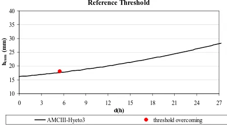
142 V. Montesarchio et al.: Rainfall thresholds: an operative case study Reference Threshold 10 15 20 25 30 35 40
0 3 6 9 12 15 18 21 24 27
d(h)
hcu
m
(m
m)
AMCIII-Hyeto3 threshold overcoming
Lead time 0.0 50.0 100.0 150.0 200.0 250.0 300.0
08/12/2005 15.30 09/12/2005 15.30 10/12/2005 15.30
date Q( m 3/s ) 0.0 1.0 2.0 3.0 4.0 5.0 hc um (m m ) threshold overcoming 9/12/2005 6.00 Qc overcoming 9/12/2005 9.30 3.5 h 10 15 20 25 30 35
0 3 6 9 12 15 18 21 24 27
d(h) hcu
m
(m
m)
AMCIII-Hyeto3 threshold overcoming
Lead time 0.0 50.0 100.0 150.0 200.0 250.0 300.0
08/12/2005 15.30 09/12/2005 15.30 10/12/2005 15.30
date Q( m 3/s ) 0.0 1.0 2.0 3.0 4.0 5.0 hc um (m m ) threshold overcoming 9/12/2005 6.00 Qc overcoming 9/12/2005 9.30 3.5 h
Fig. 8. Example of rainfall thresholds reliability evaluation.
Table 9. Rain gauges events: two-by-two contingency table.
Forecasts
Observations Warning W No Warning W0 Total
Event E 19 1 20
Non Event E0 6 2 8
Total 25 3 28
– hit rate=0.95 – false alarm rate=0.75
The mean lead time, when a warning is correctly issued, is 8.5 h, that allows to alert the emergency system. On the ba-sis of this results, for pluviometric data the threshold based forecasting system seems to have a good performance. On the other hand, the false alarm rate is quite high. False alarm were issued when there were long period of rain, but low in-tensity. So there was the time for the basin to drain the runoff without high peak discharge, even if the cumulated rainfall overcame the reference threshold. Therefore, the false alarm rate seems to depend from the infiltration dynamic, and it would be probably lower identifying differently the signifi-cant rain.
To sum up, the described threshold based forecasting sys-tem using rain gauges data works well when the rain event is short and intense, and gives problems in terms of false alarm with long low intensity events.
4.2 Reliability evaluation performed on radar data
From radar data only the November 2003 event was criti-cal for Mignone River (Fig. 9), for which a warning based on calculated thresholds is obtained. The lead time is more than 24 h. For the same event, also using rain gauges data the warning is correctly issued, even if the lead time is only of 8 h. It seems that using radar data, the warning system
November 2003 0.00 3.00 6.00 9.00 12.00 15.00 18.00
26/11 0.00 27/11 0.00 28/11 0.00 29/11 0.00 30/11 0.00
h( m m ) 0.00 50.00 100.00 150.00 200.00 250.00 300.00 Q( m 3/s )
rain gauges radar Qobserved
26/11/03 6.56.02
27/11/03 18.46.46 Radar measurement interval
Fig. 9. November 2003: rain gauges and radar data.
works better, but to completely evaluate the performance also the presence of false alarms was investigated, and results are summarised in the two-by-two contingency table (Table 10). The corresponding hit and false alarm rate are:
– hit rate=1
– false alarm rate=0.10
The results highlight a very good performance, but it is lim-ited by the characteristics of the available data set. In fact, as illustrated in par. 3.2.3, radar measurements were gen-erally not taken during flood events, and the rainfall depth estimated from radar reflectivity was generally very low, cor-responding to ordinary discharge value for critical section. Moreover, the presence of the false alarm seems due to an overestimated rainfall depth from radar data, and this proba-bly explain also the long lead time obtained. In conclusion, the threshold based forecasting system gives encouraging re-sults using radar measurements, but it is need to test the per-formance on a more consistent radar data set.
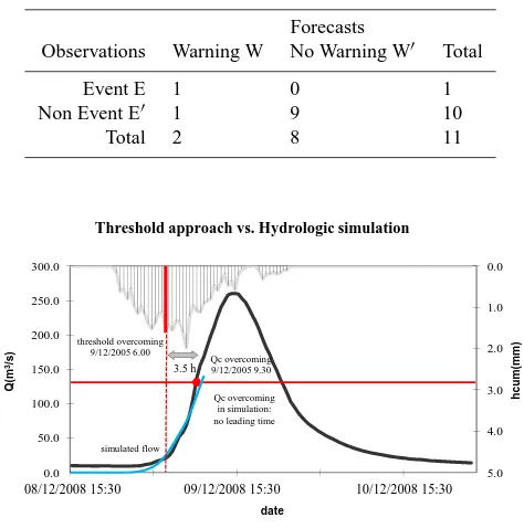
Table 10. Radar events: two-by-two contingency table.
Forecasts
Observations Warning W No Warning W0 Total
Event E 1 0 1
Non Event E0 1 9 10
Total 2 8 11
0.0
1.0
2.0
3.0
4.0
5.0 0.0
50.0 100.0 150.0 200.0 250.0 300.0
hcum(
m
m)
Q(
m
3/s
)
date
Threshold approach vs. Hydrologic simulation
threshold overcoming 9/12/2005 6.00
Qc overcoming 9/12/2005 9.30 3.5 h
simulated flow
Qc overcoming in simulation: no leading time
10/12/2008 15:30 09/12/2008 15:30
08/12/2008 15:30
Fig. 10. Comparison between threshold approach and simulation
model.
instead of comparing observed value with reference thresh-olds. Nevertheless, the rainfall threshold approach is more convenient in term of leading time. In fact, using observed precipitation for forcing rainfall runoff model can reproduce the actual situation, but not in advance: the critical discharge is simulated in the same time it is actually reached, so hy-drological simulation can not be used as forecasting system (Fig. 10).
A possibility of using calibrated hydrologic model for forecasting could be to force the model with forecasted precipitation, for different leading time, in on-line mode. Clearly, the uncertainty about the performance of the model raises by increasing the leading time and there is the need to refresh the model when new observed data are available. Thus using the calibrated hydrologic model in off-line mode as in the rainfall thresholds approach seems to be more useful in a practical warning framework.
5 Conclusions
This work shown an operative case study of a rainfall thresh-olds definition methodology. Threshold overcoming triggers the prevention and emergency system alert. Thresholds were identified by simulation from rain gauges data and then their reliability was performed on both rainfall recorded data and radar data. Using rain gauges data the thresholds hit-rate is 95%, using radar data is 100%. It follows that for Mignone River basin flood warning based on rainfall thresholds seems
to be an effective and immediate tool. However, it must be underlined that thresholds reliability was tested on few events, especially for radar data and further validation are re-quired.
Acknowledgements. The authors would like to thank Ufficio
Idro-grafico e MareoIdro-grafico of Lazio Region for providing hydrometric and pluviometric data, and Institute of Atmospheric Sciences and Climate of the National Research Council for providing radar data. The research has been partially supported by CNR-GNDCI. In addition, authors would like to thank the reviewers for their useful comments, which helped to improve the manuscript.
Edited by: G. Roth
Reviewed by: S. Manfreda and another anonymous referee
References
Annunziati, A., Focardi, A., Focardi, P., Martello, S., and Vannocci, P.: Analysis of the rainfall thresholds that induced debris flows in the area of Apuan Alps – Tuscany, Italy, Plinius Conference ’99: Mediterranean Storms, Ed. Bios., 485–493, 1999.
Agenzia Regionale per la Protezione Ambientale Piemonte, Man-uale d’uso del sistema di allertamento per situazioni di rischio idrogeologico derivanti da condizioni meteoidrologiche critiche, Direzione Regionale Servizi Tecnici di Prevenzione – Settore Meteoidrografico e reti di Monitoraggio, 2001.
Brath, A., Castellarin, A., Franchini, M., and Galeati, G.: Estimat-ing the index flood usEstimat-ing indirect methods, Hydrolog. Sci. J., 46(3), 399–418, 2001.
Carpenter, T. M., Sperfslage J. A., Georgakakos K. P., Sweeney, T., and Fread, D. L.: National threshold runoff estimation utiliz-ing GIS in support of operational flash flood warnutiliz-ing systems, J. Hydrol., 224, 21–44, 1999.
Crosta, G. B. and Frattini, P.: Rainfall thresholds for soil slip and debris flow triggering, Proceedings of the EGS 2nd Plinius Con-ference on Mediterranean Storms, Ed. Bios., 463–488, 2000. Dalrymple, T.: Flood frequency analyses, Water Supply Paper
1543-A, US Geol. Survey, Reston, Virginia, USA, 1960. Georgakakos, K. P.: Analytical results for operational flash flood
guidance, J. Hydrol., 317, 81–103, 2006.
Georgakakos, K. P.: Real time prediction for flood warning and management, U.S.-Italy Research Workshop on the Hydromete-orology, Impacts, and Management of Extreme Floods Perugia (Italy), November 1995, 1995.
Hydrologic Engineering Center: Geospatial Hydrologic Modeling Extension HEC-GeoHMS: User’s Manual, U.S. Army Corps of Engineers, Davis, CA, 281 pp., 2003a.
Hydrologic Engineering Center: Hydrologic Modeling System (HEC-HMS): Release Notes, U.S. Army Corps of Engineers, Davis, CA, USA, 280 pp., 2003b.
Kirkby, M. J.: Tests of the random network model and its applica-tion to basin hydrology, Earth Surf. Processes, 1, 197–212, 1976. Koutsoyiannis, D. and Xanthopoulos, T.: Engineering Hydrology, Edition 3, National Technical University of Athens, Athens, Greece, 418 pp., 1999.
Karunanithi, N., Grenney, W., Whitley, D. and Bovee, K.: Neural networks for river flow prediction, J. Comput. Civil Eng., 8(2), 201–220, 1994.
Lombardo F., Napolitano F., Russo F., Scialanga G., Baldini, L., and Gorgucci, E.: Rainfall estimation and ground clutter rejection with dual polarization weather radar, Advances in Geosciences, 7, 127–130, 2006.
Mancini, M., Mazzetti P., Nativi, S., Rabuffetti, D., Ravazzani, G., Amadio, P., and Rosso, R.: Definizione di soglie pluviometriche di piena per la realizzazione di un sistema di allertamento in tempo reale per il bacino dell’Arno a monte di Firenze, Proc. XXVII Convegno di idraulica e Costruzione Idrauliche, Italy, 2, 497–505, 2002.
Martina, M. L. V., Todini, E., and Libralon, A.: A Bayesian deci-sion approach to rainfall thresholds based flood warning, Hydrol. Earth Syst. Sci., 10, 413–426, 2006,
http://www.hydrol-earth-syst-sci.net/10/413/2006/.
Mason, S. J. and Graham, N. E.: Conditional Probabilities, Rel-ative Operating Characteristics and RelRel-ative Operating Levels, Weather Forecast., 14, 713–725, 1999.
Mesa, O. J. and Mifflin, E. R.. On the relative role of hillslope and network geometry in hydrologic response, in: Scale Problems in Hydrology, D. Reidel, edited by: Gupta, V., Rodriguez-Iturbe, I., and Wood, E., 1–17, Dordrecht, The Netherlands, 1986. Naden, P. S: Spatial variability in flood estimation for large
catch-ments: the exploitation of channel network structure, J. Hydrol. Sci., 37(1–2), 53–71, 1992.
Nash, J. E. and Sutcliffe, J. V.: River flow forecasting through con-ceptual models 1: a discussion of principles, J. Hydrol., 10(3), 282–290, 1970.
Neary, D. G. and Swift, L. W.: Rainfall thresholds for trigger-ing a debris flow avalanchtrigger-ing event in the southern Appalachian Mountains, Rew. Eng. Geol., 7, 81–95, 1987.
Peters, J. C. and Easton, D. J.: Runoff Simulation Using Radar Rainfall Data, Water Resour. Bull., 32(4), 753–760, 1996. Pilgrim, D. H. and Cordery, I.: Flood runoff, in: Handbook of
hy-drology, edited by: Maidment, D. R., McGraw-Hill, New York, NY, USA, 9, 1–42, 1993.
Rodriguez-Iturbe, I. and Valdes, J. B.: The geomorphologic struc-ture of hydrologic response, Water Resour. Res., 15(6), 1409– 1420, 1979.
Rosso, R.: Manuale di Protezione Idraulica del Territorio, Cusl, Mi-lano, Italy, 2002.
Russo, F., Napolitano, F., and Gorgucci, E.: Rainfall monitoring systems over an urban area: the city of Rome, Hydrol. Process., 19(5), 1007–1019, 2005.
Soil Conservation Service: National engineering handbook, Cross section 4: Hydrology, US Department of Agriculture, Spring-field, VA, USA, 1971.
Soil Conservation Service: Urban hydrology for small watersheds, Technical Release 55, US Department of Agriculture, Spring-field, VA, USA, 1986.
Regione Lazio website (http://www.regione.lazio.it), Regione Lazio Dipartimento Territorio, Piano di tutela delle acque, Bacini idro-grafici e schede riassuntive per bacino, 170 pp., 2006.
Regione Lazio website (http://www.regione.lazio.it), Regione Lazio Dipartimento Territorio, Piano di tutela delle acque, Geologia, Idrogeologia e Vulnerabilit del territorio, 98 pp., 2006.