Dual Methods for Optimal Allocation
of Telecommunication Network Resources
with Several Classes of Users
I.V. Konnov1, A. Yu. Kashuba1and E.J. Laitinen2,*
1 Department of System Analysis and Information Technologies, Kazan Federal University, Kazan 420008,
Russia; [email protected]
2 Scientific Research Laboratory "Computational Technologies and Computer Modeling", Institute of
Computational Mathematics and Information Technologies, Kazan Federal University, Kazan 420008, Russia; [email protected]
3 Faculty of Science, Research Unit of Mathematical Sciences, P.O.Box 8000 FI-90014 University of Oulu,
Finland; [email protected]
* Correspondence: [email protected]; Tel.: +358 50 3504953
Abstract: We consider a general problem of optimal allocation of limited resources in a wireless telecommunication network. The users are divided into several different groups (or classes), which correspond to different levels of service. The network manager must satisfy these different users requirements. This approach leads to a convex optimization problem with balance and capacity constraints. We present several decomposition type methods to find a solution of this problem, which exploit its special features. We suggest to apply first the dual Lagrangian method with respect to the total capacity constraint, which gives the one-dimensional dual problem. However, calculation of the value of the dual cost function requires solution of several optimization problems. Our methods differ in approaches of solution of these auxiliary problems. We compare the performance of the suggested methods on several series of test problems. They show rather satisfactory convergence. Nevertheless, proper decomposition technique enhance the convergence essentially.
Keywords: telecommunication networks, wireless networks, service levels, resource allocation, optimization problem, decomposition methods, Lagrange duality.
1. Introduction
Efficient allocation of limited communication networks resources requires flexible mechanisms, which are based on proper mathematical models, since the custom fixed allocation rules may lead to congestion effects and additional expenses from the inefficient utilization of network resources; see
e.g. [1]–[3]. In particular, spectrum sharing is now one of the most critical issues and various adaptive
mechanisms for allocation of resources in wireless telecommunication networks have been suggested. Most papers in this field are devoted to game-theoretic models and implementation of decentralized
iterative methods for finding the Nash equilibrium points or their generalizations; see e.g. [4,5]. At the
same time, various optimization based mechanisms are also suggested; see e.g. [3,5–7]. Treatment of
these very complicated systems is often based on a proper decomposition approach, which can involve zonal, time, frequency and other decomposition techniques.
In [8]–[13], several optimal resource allocation problems in telecommunication networks and
proper zonal decomposition based methods were suggested. They assumed that the network manager can satisfy all the varying users requirements or can buy additional volumes of the resource. This approach leads to constrained convex optimization problems for some selected time period. However, these models do not take into account possible differentiation of users with respect to service levels, which yields different service costs and somewhat different optimization problems.
In this paper, we just consider problems of optimal allocation of a homogeneous resource in a telecommunication network with the differentiation of users. In such a way, we give a new formulation of this problem as an optimization problem and present several dual decomposition type methods for the affine and convex cases. We compare the performance of the suggested methods on several series of test problems.
2. Problem formulation
Let us consider a single telecommunication network with nodes (users). A network manager
offers usersmlevels of network service (classes), which is reflected by expenses and prices. Within
some selected time period, the network manager can offer a limited total amountCof a homogeneous
resource of the network. An amount of resource allocated to thei-th class service is supposed to be
equal toϕi(xi)ifxiis an unknown consumed traffic volume at this level (0≤xi ≤ βi). The cost of
implementation (network expense) of the amountxiof thei-th service level is supposed to be equal to
µi(xi). Each user can choose only one level of service. LetN={1, . . . ,n}denote a set of users, andNi
a set of users of thei-th class (level) fori=1, . . . ,m. Letyjdenote the unknown traffic volume offered
to thej-th user with 0≤ yj ≤αjandηj(yj)is the fee (incentive) value paid by thej-th user for this
traffic. If all the users are attributed to the classes, we can calculate the total traffic volume for eachi-th
level as follows:
xi=
∑
j∈Niyj.
The general problem of the network manager is to find an optimal allocation of the limited homogeneous resource among the users in order to maximize the total payment received from the users and minimize the total network implementation expenses. This problem is now formulated as follows:
max (x,y)∈W,∑m
i=1ϕi(xi)≤C
→ f(x,y), (1)
where
f(x,y) =
m
∑
i=1 "
∑
j∈Ni
ηj(yj)−µi(xi) #
(2)
and
W=
(
(x,y) xi=
∑
j∈Ni
yj, 0≤yj ≤αj, j∈Ni, 0≤xi≤βi,i=1, . . . ,m )
. (3)
In what follows we shall suppose that all the functionsµi(xi),ϕi(xi)and−ηj(yj)are convex, then
(1)–(3) is a convex optimization problem.
3. Solution methods
It is well known that there exist a great number of efficient solution methods for convex
optimization problems; see e.g. [14,15]. However, due to large dimensionality and inexact data
of the optimal resource allocation problems in telecommunication networks one can meet serious difficulties when solving these problems with custom general iterative solution methods. In order to
create an efficient method just for problem (1)–(3), we have to take into account its separability and
apply certain decomposition approach. Moreover, the standard duality scheme using the Lagrangian function with respect to all the functional constraints leads to the multi-dimensional dual optimization
problem. We will apply another approach, which was suggested in [10,16] and leads to solution of
one-dimensional problems.
Let us first define the Lagrange function of problem (1)–(3) as follows:
L(x,y,λ) = f(x,y)−λ
m
∑
i=1
ϕi(xi)−C !
This means we will utilize the Lagrangian multiplierλonly for the total resource bound. We can now
replace problem (1)–(3) with its dual:
min
λ≥0 →ψ(λ), (4)
where
ψ(λ) = max
(x,y)∈WL(x,y,λ) =λC+(xmax,y)∈W m
∑
i=1 "
∑
j∈Ni
ηj(yj)−(µi(xi) +λϕi(xi)) #
.
By duality (see e.g. [14,15]), problems (1)–(3) and (4) have the same optimal value. But solution of (4)
can be found by one of well-known single-dimensional optimization algorithms; see e.g. [15]. The
main problem is to implement these algorithms properly.
In order to calculate the value ofψ(λ)we have to solve the inner problem:
max (x,y)∈W→
m
∑
i=1 "
∑
j∈Ni
ηj(yj)−(µi(xi) +λϕi(xi)) #
.
This problem clearly decomposes intomindependent class problems
max→
∑
j∈Ni
ηj(yj)−(µi(xi) +λϕi(xi)), (5)
subject to
xi =
∑
j∈Niyj, 0≤yj ≤αj, j∈ Ni, 0≤xi ≤βi, fori=1, . . . ,m. (6)
Our methods for problem (1)–(3) will differ in approaches to problem (5)–(6).
We first describe the decomposition approach, which follows in general that from [8–10]. Denote
byνi(xi)the optimal value of thei-th service optimization problem:
max→
∑
j∈Ni
ηj(yj) (7)
subject to
∑
j∈Ni
yj=xi, 0≤yj ≤αj,j∈Ni. (8)
Then (5)–(6) reduces to the one-dimensional problem:
min 0≤xi≤βi
→νi(xi)−µi(xi)−λϕi(xi). (9)
It is easy to see thatνi(xi)is a convex, but non differentiable function in general.
Thus, the initial problem (1)–(3) is replaced by its one-dimensional dual (4) with the cost function
ψ(λ), such that calculation of its value reduces to solution ofmindependent problems of form (5)–(6),
whose calculation again reduces to solution of one-dimensional problems of form (9).
However, each functionνiis given algorithmically, i.e., via solution of problem (7)–(8). In the
general case we can apply again a dual type method to find the value ofνi(xi). Let us to introduce the
the Lagrange function
˜
Lj(y,θi) =
∑
j∈Niηj(yj)−θi "
∑
j∈Ni
yj−xi #
,
and then to solve the one-dimensional dual:
min θi≥0
where
ζi(θi) =θixi+
∑
j∈Nimax 0≤yj≤αj
[ηj(yj)−θiyj].
Therefore, we can use here only algorithms for a set of hierarchical one-dimensional problems. Let us
denote this method as(DML).
Note that this approach involves several levels of hierarchical problems requiring certain concordance in the accuracies of the solution of all these problems, besides, each solution of one upper level problem requires solution of all the lower level problems many times, which entails large computational costs. However, they can be reduced for some special types of functions.
For instance, consider the case where the functionsηj(yj),j∈Niare affine, whereas the functions
ϕi(xi)andµi(xi)are convex and differentiable. Then we can find an exact solution of problems (7)–(8)
by a simple ordering algorithm in a finite number of iterations; see [17] for more detail.
Next, consider the particular case where all the functionsηj(yj),µi(xi), andϕi(xi)are affine, i.e.
ηj(yj) =ηj,1yj+ηj,0, ηj,1>0,j∈Ni,i=1, . . . ,m,
µi(xi) =µi,1xi+µi,0, µi,1>0,i=1, . . . ,m, (10)
ϕi(xi) =ϕi,1xi+ϕi,0, ϕi,1>0,i=1, . . . ,m.
Then the cost function in (5) can be rewritten equivalently as
ηj,1yj−(µi,1+λϕi,1)xi.
This means that problems (5)–(6) reduces to a two-side auction market with fixed prices (see [17]) and
also is solved in a finite number of iterations by a simple ordering algorithm; see also [11,16]. Let us
denote this method as(SDM).
We can extend this approach to the case where the functionsηj(yj)are affine as in (10), whereas
the functionsϕi(xi)andµi(xi)are only convex and differentiable. This means that the prices (marginal
utilities)ηj,1of the users are fixed, but the marginal expenses and prices depend on volumes, so that
they are non-decreasing. Sety(i) = (yj)j∈Niand
Wi = (
(xi,y(i)) xi =
∑
j∈Ni
yj, 0≤yj ≤αj, j∈ Ni, 0≤xi ≤βi )
.
The necessary and sufficient optimality condition for problem (5)–(6) is now written in the form of the
variational inequality: find(x¯i, ¯y(i))∈Wisuch that
(µ0i(x¯i) +λϕ0i(x¯i))(xi−x¯i)−
∑
j∈Niηj,1(yj−y¯j)≥0, ∀(xi,y(i))∈Wi. (11)
This is a two-sided market equilibrium problem with one seller and several buyers; see e.g. [17]. It is
equivalent to the problem of finding a vector(x¯i, ¯y(i))∈Wiand a cutting price ¯pisuch that
µ0i(x¯i) +λϕ0i(x¯i)
≥ p¯i, if ¯xi =0,
= p¯i, if ¯xi ∈[0,βi],
≤ p¯i, if ¯xi =βi,
(12)
and
ηj,1
≤ p¯i, if ¯yj=0,
= p¯i, if ¯yj∈[0,αj],
≤ p¯i, if ¯yj=αj.
Since buyers prices are fixed, we can re-arrange them to be non-increasing and then find easily an
intersection point of the staircase-wise inverse common demand and offer priceµ0i(xi) +λϕ0i(xi)lines;
see also [11]. Therefore, the exact solution of problem (11) or (5)–(6) can be also found directly by
simple ordering type algorithms applying to (12)–(13) although (5)–(6) contains a non-linear function.
In other words, calculation of values ofψ(λ)can be now accomplished by several independent simple
ordering type algorithms. Notice that the re-arrangement of bid pricesηj,1in each class should be made
only one time that reduces the computational expenses essentially in comparison with the general
duality approach. Let us denote this method also as(SDM).
We now again consider the general case where all the functionsµi(xi),ϕi(xi), and−ηj(yj)are
convex and differentiable. For these problems there exist many rather efficient solution methods; see
e.g. [18] and references therein. In view of the above properties we can replace each problem (5)–(6)
with a sequence of linearized problems of the form:
min (xi,y(i))∈Wi
→ "
(µ0i(xki) +λϕ0i(xki))xi−
∑
j∈Niη0j(ykj)yj #
(14)
if we apply the custom conditional gradient method(CGM)as suggested in [19]. For the sake of clarity,
we describe(CGM)applied to the general optimization problem
min
v∈V →φ(v),
whereVis a convex closed set,φis a convex and differentiable function.
(CGM)Take an arbitrary initial pointv0∈Vand a numberδ>0. At thes-th iteration,s=0, 1, . . .,
we have a pointvs ∈Vand calculateus ∈Vas a solution of the linear programming problem
min u∈V → hφ
0(vs),ui. (15)
Then we setps =us−vs. Ifkpsk ≥ −δ, stop, we have an approximate solution. Otherwise we find
the next iteratevs+1as follows:
vs+1=σsus+ (1−σs)vs,
whereσs∈(0, 1)is a step-size parameter.
In particular, we can utilize the inexact line search procedure: Findmas the minimal non-negative
integer such that
φ(vs+θmps)≤φ(vs) +αθmhφ0(vs),psi,
for someα∈(0, 1)andθ∈(0, 1), and setσs =θm; see [20].
It is easy to see that (15) gives then (14). Hence, (14) can be solved by simple ordering type
algorithms as in (SDM). We denote this method as (CGDM). However, this approach requires
application of(CGM)many times at each iteration of a single-dimensional optimization algorithm
applied to the upper problem (4). At the same time, we can apply the same dual decomposition
method to problem (5)–(6). For the sake of simplicity, we rewrite (5)–(6) as follows:
max (x,y)∈D
→
∑
j∈J
where
D=
(
(x,y) x=
∑
j∈J
yj, 0≤yj≤αj, j∈ J, 0≤x≤β
)
,
x=xi, y= (yj)j∈J, J= Ni, β=βi,
u(x) =µi(x) +λϕi(x).
Letg(x) =u0(x)andwj(yj) =ηj0(yj). The necessary and sufficient optimality condition for problem
(16) is given in (11) and re-written now as the variational inequality: find(x¯, ¯y)∈Dsuch that
g(x¯)(x−x¯)−
∑
j∈J
wj(y¯j)(yj−y¯j)≥0,∀(x,y)∈ D.
The optimality conditions in (12)–(13) have the form: find(x¯, ¯y)∈Dandp∗such that
g(x¯)
≥p∗, if ¯xi=0,
=p∗, if ¯xi∈[0,β],
≤p∗, if ¯xi=β,
(17)
and
wj(y¯j)
≤p∗, if ¯yj=0,
=p∗, if ¯yj∈[0,αj],
≥p∗, if ¯yj=αj;
forj∈J. (18)
Following the dual approach, we write the Lagrange function of problem (16) with the negative
sign:
M(x,y,p) = u(x)−
∑
j∈J
ηj(yj)−p x−
∑
j∈Jyj !
= (u(x)−px)−
∑
j∈J
(ηj(yj)−pyj).
In order to find a value of the dual cost function
θ(p) = min
x∈[0,β],y∈[0,α]
M(x,y,p),
whereα= (αj)j∈J, we have to solve the one-dimensional problems:
min 0≤x≤β
→(u(x)−px),
and
min 0≤yj≤αj
→(−ηj(yj) +pyj), forj∈ J.
For the sake of simplicity, we also suppose that the functionsu and−ηj are strictly convex. Then
solutions of the above problems denoted byx(p)andyj(p),j∈ J, respectively, are defined uniquely. It
follows that the functionθ(p)is concave and differentiable with the derivative
θ0(p) =
∑
j∈J
Besides, the one-dimensional dual problem
max
p →θ(p) coincides with the simple equation
θ0(p) =0, (19)
whereθ0(p)is non-increasing. Therefore, ifp∗is the solution of (19), then we can find the solution of
problem (16) from (17)–(18) by settingp=p∗, which gives a solution of the initial problem (5)–(6).
In order to find a solution of (17) we can apply bisection type algorithms. Letγ0 = g(0)and
γ00 =g(β). Thenγ0 <γ00. Letδ0j =w(0)andδ00j =w(αj). If we setp00=max j∈J δ
0
jandp0=γ0, then the
casep00≤p0gives immediately the zero solutions in accordance with (17)–(18). So we can consider
only the non-trivial case wherep0 < p00. Then by (17)–(18) we must haveθ0(p0)≥0 andθ0(p00)≤0.
These properties enable us to utilize the simplest bisection algorithm; see e.g. [12,13].
Algorithm (BS). Given an accuracyε>0 and the initial segment[p0,p00], we take ˜p=0.5(p0+p00),
calculateθ0(p˜). Then we setp0= p˜ifθ0(p˜)>0 andp0 =p˜otherwise, until(p00−p0)<ε.
Also, if all the functions are quadratic, we can utilize a heuristic method similar to that in [12].
Algorithm (SQ). Letωj = ηj,1+λϕi,1. Define Ja = {j∈ J|ωj > p0}, sety∗j =0 for j∈/ Jaand
re-arrange the indices inJato have the descending order for the values ofωj. Then find two sequential
indicesjlandjl+1inJasuch that∆l<0 and∆l+1>0, where
∆l = l
∑
s=1
yjs(ωjl)−xωjl).
Then findp∗such thatθ0(p∗) =0 in the segment[ωjl,ωjl+1].
4. Numerical experiments
The methods were implemented in C++ with a PC with the following facilities: Intel(R) Core(TM) i7-4500, CPU 1.80 GHz, RAM 6 Gb.
The initial interval for the dual variableλwere chosen as [0,1000]. The parametersβi(i=1, . . . ,m)
andαj(j ∈ Ni,i = 1, . . . ,m)were chosen as values of trigonometric functions in [1, 51]and[1, 2],
respectively. We set the constantCto be equal 1000. The number of classes was varied from 3 to 45, the
number of users was varied from 210 to 1010. Users were distributed among classes either uniformly or according to the normal distribution.
We considered the following kinds of functions in test problems of form (1)–(3):
[Case L]All the functionsµi(xi),ϕi(xi), andηj(yj)are affine;
[Case QL]All the functionsηj(yj)are affine, all the functionsµi(xi)andϕi(xi)are quadratic;
[Case EQ]All the functions−ηj(yj)are convex quadratic, all the functionsµi(xi)and ϕi(xi)are convex exponential;
[Case Q]All the functions−ηj(yj),µi(xi), andϕi(xi)are convex quadratic;
[Case E]All the functions−ηj(yj),µi(xi), andϕi(xi)are convex exponential;
[Case LG]All the functions−ηj(yj),µi(xi), andϕi(xi)are convex logarithmic.
1. Linear functions
ηj(yj) =ηj,1yj+ηj,0,ηj,1>0, j=1, . . . ,J,
µi(xi) =µi,1xi+µi,0,µi,1>0, i=1, . . . ,m,
ϕi(xi) =ϕi,1xi+ϕi,0,ϕi,1>0, i=1, . . . ,m, where
ηj,1=2|sin(j+1)|+1,ηj,0=2|sin(2j)|+1, j=1, . . . ,J,
µi,1=|cos(i)|+1,µi,0=2|cos(2i)|+1, i=1, . . . ,m,
ϕi,1=µi,1,ϕi,0=µi,0, i=1, . . . ,m.
2. Quadratic functions
ηj(yj) =0.5ηj,2y2j +ηj,1yj,ηj,2<0, j=1, . . . ,J,
µi(xi) =0.5µi,2x2i +µi,1xi,µi,2>0, i=1, . . . ,m,
ϕi(xi) =0.5ϕi,2x2i +ϕi,1xi,ϕi,2>0, i=1, . . . ,m, where
ηj,2=−4|cos(2j−1)| −4,ηj,1=|sin(j+1)|+1, j=1, . . . ,J,
µi,2=|sin(2i)|+1,µi,1=|cos(i)|+3, i=1, . . . ,m,
ϕi,2=µi,2,ϕi,1=µi,1, i=1, . . . ,m. 3. Exponential functions
ηj(yj) =ηj,0+ηj,1yj−ηj,2eηj,3yj,ηj,1,ηj,2>0, j=1, . . . ,J,
µi(xi) =µi,0eµi,1xi,µi,1,µi,0>0, i=1, . . . ,m,
ϕi(xi) =ϕi,0eϕi,1xi,ϕi,1,ϕi,0>0, i=1, . . . ,m, where
ηj,3=|sin(j+1)|+1,ηj,2=2|sin(2j)|+1,
ηj,1=2|sin(j+1)|+8,ηj,0=2|sin(2j)|+9, j=1, . . . ,J,
µi,1=|cos(i)|+1,µi,0=2|cos(2i)|+1, i=1, . . . ,m,
ϕi,1=µi,1,ϕi,0=µi,0, i=1, . . . ,m. 4. Logarithmic functions
ηj(yj) =ηj,2ln(1+ηj,0+ηj,1yj),ηj,0,ηj,1,ηj,2>0, j=1, . . . ,J,
µi(xi) =µi,0+µi,1xi−ln(1+µi,2+µi,3xi),µi,1,µi,2,µi,3>0, i=1, . . . ,m,
where
ηj,0=2|sin(2j)|,ηj,1=|sin(j+1)|+1,
ηj,2=3|sin(2j)|+1, j=1, . . . ,J,
µi,0=2|cos(2i)|+1,µi,1=|cos(i)|+1,
µi,2=2|cos(2i)|,µi,3=|cos(i)|+1, i=1, . . . ,m,
ϕi,0=µi,0,ϕi,1=µi,1,ϕi,2=µi,2,ϕi,3=µi,3, i=1, . . . ,m.
For all the methods of solving problem (1)–(3) the accuracy of solution of upper dual problem (4)
was varied from 10−1to 10−4. The accuracy of solution of lower level problems was fixed to be equal
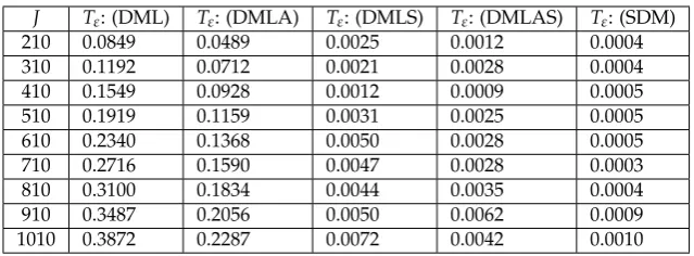
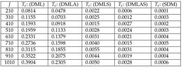
10−2. For each set of the parameters 50 tests were made. In the tables,Tεdenotes the total processor
time in seconds. The averaged results of computations for Case L are given in Tables1–3, for Case QL
are given in Tables4–6, for Case Q are given in Tables7–9, for Case EQ are given in Tables10–12, for
Case E are given in Tables13–15, for Case LG are given in Tables16–18.
Together with the three basic methods for problem (1)–(3) named(DML),(CGDM), and(BS), we
tested also their modifications adjusted mainly to some particular classes of problems. We applied
the method(DML)with adaptive strategy of choosing the inner accuracies and named it(DMLA).
In the case where the functionsηj(yj)are affine, we applied also the simplified versions of these
methods named(DMLS)and(DMLAS), respectively. They solve auxiliary problems (7)–(8) by a
simple ordering algorithm in a finite number of iterations and require only one arrangement of buyers’
prices. Methods(DML),(DMLA),(DMLS),(DMLAS)and(SDM)were applied for cases L and QL,
where(DMLS)and(DMLAS) showed better performance than(DML) and(DMLA), but(SDM)
showed the best results here.
Table 1.Results for Case L withJ=510,m=25
ελ Tε: (DML) Tε: (DMLA) Tε: (DMLS) Tε: (DMLAS) Tε: (SDM) 10−1 0.1680 0.0897 0.0025 0.0024 0.0003 10−2 0.1919 0.1159 0.0031 0.0025 0.0004 10−3 0.2371 0.1597 0.0047 0.0028 0.0009 10−4 0.2728 0.2128 0.0062 0.0046 0.0012
Table 2.Results for Case L withm=25,ε=10−2
Table 3.Results for Case L withJ=510,ε=10−2
m Tε: (DML) Tε: (DMLA) Tε: (DMLS) Tε: (DMLAS) Tε: (SDM) 3 0.1781 0.0988 0.0024 0.0021 0.0004 9 0.1966 0.1130 0.0019 0.0012 0.0004 15 0.1976 0.1156 0.0018 0.0009 0.0001 21 0.2004 0.1157 0.0018 0.0018 0.0003 27 0.1953 0.1140 0.0027 0.0012 0.0007 33 0.1958 0.1153 0.0028 0.0021 0.0007 39 0.1994 0.1174 0.0024 0.0022 0.0004 45 0.2010 0.1175 0.0040 0.0022 0.0005
Table 4.Results for Case QL withJ=510,m=25
ελ Tε: (DML) Tε: (DMLA) Tε: (DMLS) Tε: (DMLAS) Tε: (SDM) 10−1 0.1665 0.0906 0.0025 0.0021 0.0003 10−2 0.1959 0.1133 0.0028 0.0024 0.0004 10−3 0.2346 0.1603 0.0049 0.0028 0.0006 10−4 0.2762 0.2144 0.0053 0.0041 0.0007
Table 5.Results for Case QL withm=25,ε=10−2
J Tε: (DML) Tε: (DMLA) Tε: (DMLS) Tε: (DMLAS) Tε: (SDM) 210 0.0814 0.0478 0.0022 0.0006 0.0001 310 0.1155 0.0703 0.0025 0.0012 0.0003 410 0.1593 0.0918 0.0015 0.0027 0.0002 510 0.1959 0.1133 0.0028 0.0024 0.0003 610 0.2331 0.1379 0.0031 0.0021 0.0004 710 0.2736 0.1598 0.0040 0.0015 0.0005 810 0.3115 0.1855 0.0055 0.0031 0.0004 910 0.3522 0.2075 0.0044 0.0019 0.0004 1010 0.3904 0.2305 0.0050 0.0028 0.0006
Table 6.Results for Case QL withJ=510,ε=10−2
m Tε: (DML) Tε: (DMLA) Tε: (DMLS) Tε: (DMLAS) Tε: (SDM) 3 0.1753 0.0984 0.0056 0.0009 0.0001 9 0.1953 0.1153 0.0031 0.0016 0.0003 15 0.1981 0.1187 0.0031 0.0019 0.0002 21 0.1965 0.1196 0.0021 0.0009 0.0002 27 0.1924 0.1141 0.0025 0.0019 0.0001 33 0.1958 0.1163 0.0034 0.0025 0.0003 39 0.1977 0.1162 0.0041 0.0015 0.0001 45 0.1964 0.1158 0.0031 0.0015 0.0006
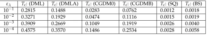
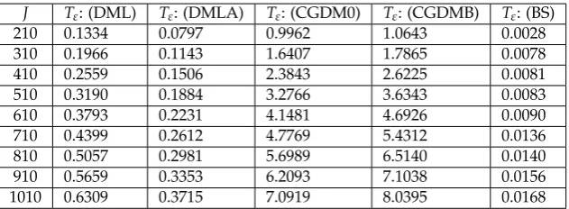
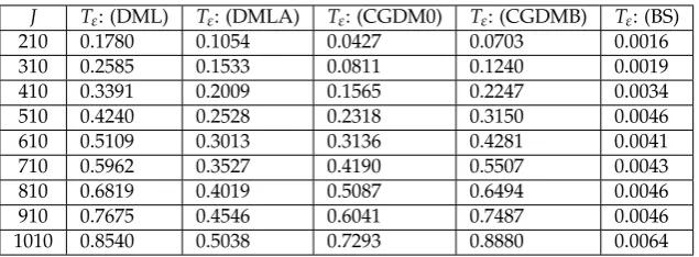
Next, in the nonlinear case, we applied(CGDM), where(CGDM0)denotes the version with zero
initial point for any(CGM),(CGDMB)denotes the version with taking the initial point for any(CGM)
in the boundary of the feasible set. We utilized these methods with the inexact line search procedure.
Here(BS)and(SQ)showed the best performance, and the results of(CGDM0)and(CGDMB)were
better than those of(DML)and(DMLA).
Table 7.Results for Case Q withJ=510,m=25
ελ Tε: (DML) Tε: (DMLA) Tε: (CGDM0) Tε: (CGDMB) Tε: (SQ) Tε: (BS) 10−1 0.2815 0.1488 0.0283 0.0762 0.0012 0.0018 10−2 0.3271 0.1929 0.0474 0.1116 0.0015 0.0019 10−3 0.3909 0.2669 0.1049 0.1919 0.0026 0.0040 10−4 0.4575 0.3570 0.1486 0.2534 0.0028 0.0058
Table 8.Results for Case Q withm=25,ε=10−2
J Tε: (DML) Tε: (DMLA) Tε: (CGDM0) Tε: (CGDMB) Tε: (SQ) Tε: (BS) 210 0.1377 0.0833 0.0113 0.0367 0.0006 0.0009 310 0.2004 0.1179 0.0208 0.0580 0.0012 0.0019 410 0.2657 0.1564 0.0321 0.0828 0.0009 0.0018 510 0.3271 0.1929 0.0474 0.1116 0.0015 0.0019 610 0.3900 0.2302 0.0641 0.1396 0.0027 0.0030 710 0.4540 0.2682 0.0728 0.1568 0.0019 0.0034 810 0.5181 0.3052 0.0862 0.1804 0.0022 0.0028 910 0.5809 0.3437 0.0934 0.1960 0.0028 0.0043 1010 0.6434 0.3793 0.1021 0.2110 0.0025 0.0046
Table 9.Results for Case Q withJ=510,ε=10−2
m Tε: (DML) Tε: (DMLA) Tε: (CGDM0) Tε: (CGDMB) Tε: (SQ) Tε: (BS) 3 0.3028 0.1663 0.0465 0.0937 0.0003 0.0031 9 0.3203 0.1881 0.0546 0.0986 0.0015 0.0021 15 0.3250 0.1956 0.0668 0.1205 0.0012 0.0019 21 0.3278 0.1952 0.0541 0.1131 0.0015 0.0022 27 0.3271 0.1957 0.0462 0.1075 0.0012 0.0028 33 0.3300 0.1946 0.0462 0.1111 0.0006 0.0034 39 0.3353 0.1972 0.0365 0.1037 0.0003 0.0028 45 0.3337 0.1974 0.0333 0.0968 0.0006 0.0021
Methods(DML),(DMLA),(CGDM0),(CGDMB), and(BS)were applied for cases EQ, E, and
LG. Here(BS)showed the essentially better results than the other methods. Also,(DMLA)showed
better performance than(DML),(CGDM0), and(CGDMB)in most test experiments.
Table 10.Results for Case EQ withJ=510,m=25
Table 11.Results for Case EQ withm=25,ε=10−2
J Tε: (DML) Tε: (DMLA) Tε: (CGDM0) Tε: (CGDMB) Tε: (BS) 210 0.1382 0.0845 0.0293 0.0824 0.0030 310 0.2028 0.1187 0.0674 0.1753 0.0018 410 0.2644 0.1555 0.1127 0.2857 0.0021 510 0.3281 0.1938 0.1497 0.4153 0.0043 610 0.3906 0.2294 0.1693 0.5499 0.0053 710 0.4510 0.2669 0.2031 0.6742 0.0050 810 0.5161 0.3075 0.2312 0.7656 0.0059 910 0.5766 0.3449 0.2718 0.8646 0.0097 1010 0.6421 0.3819 0.3184 0.9579 0.0085
Table 12.Results for Case EQ withJ=510,ε=10−2
m Tε: (DML) Tε: (DMLA) Tε: (CGDM0) Tε: (CGDMB) Tε: (BS)
3 0.3035 0.1671 0.0762 0.3703 0.0040
9 0.3188 0.1871 0.0746 0.3753 0.0030
15 0.3231 0.1932 0.1228 0.4345 0.0046 21 0.3278 0.1949 0.1459 0.4269 0.0053 27 0.3278 0.1924 0.1193 0.3479 0.0047 33 0.3309 0.1955 0.1215 0.3411 0.0041 39 0.3303 0.1981 0.1124 0.2996 0.0053 45 0.3325 0.1949 0.1166 0.2928 0.0052
Table 13.Results for Case E withJ=510,m=25
ελ Tε: (DML) Tε: (DMLA) Tε: (CGDM0) Tε: (CGDMB) Tε: (BS) 10−1 0.2787 0.1468 1.9862 2.3146 0.0071 10−2 0.3190 0.1884 3.2766 3.6343 0.0083 10−3 0.3887 0.2642 5.1906 5.6561 0.0146 10−4 0.4446 0.3522 6.9235 7.4660 0.0175
Table 14.Results for Case E withm=25,ε=10−2
Table 15.Results for Case E withJ=510,ε=10−2
m Tε: (DML) Tε: (DMLA) Tε: (CGDM0) Tε: (CGDMB) Tε: (BS)
3 0.2981 0.1662 2.4191 2.8496 0.0072
9 0.3128 0.1828 2.8231 3.2803 0.0068
15 0.3203 0.1896 3.6925 4.1387 0.0106 21 0.3216 0.1918 3.6565 4.0279 0.0103 27 0.3225 0.1881 3.2027 3.5053 0.0089 33 0.3247 0.1907 1.7065 1.9672 0.0109 39 0.3278 0.1916 2.9506 3.2169 0.0099 45 0.3264 0.1906 2.9452 3.1939 0.0113
Table 16.Results for Case LG withJ=510,m=25
ελ Tε: (DML) Tε: (DMLA) Tε: (CGDM0) Tε: (CGDMB) Tε: (BS) 10−1 0.3617 0.1921 0.1438 0.2213 0.0028 10−2 0.4240 0.2528 0.2318 0.3150 0.0046 10−3 0.5090 0.3452 0.3934 0.5133 0.0051 10−4 0.5900 0.4627 0.5259 0.6784 0.0053
Table 17.Results for Case LG withm=25,ε=10−2
J Tε: (DML) Tε: (DMLA) Tε: (CGDM0) Tε: (CGDMB) Tε: (BS) 210 0.1780 0.1054 0.0427 0.0703 0.0016 310 0.2585 0.1533 0.0811 0.1240 0.0019 410 0.3391 0.2009 0.1565 0.2247 0.0034 510 0.4240 0.2528 0.2318 0.3150 0.0046 610 0.5109 0.3013 0.3136 0.4281 0.0041 710 0.5962 0.3527 0.4190 0.5507 0.0043 810 0.6819 0.4019 0.5087 0.6494 0.0046 910 0.7675 0.4546 0.6041 0.7487 0.0046 1010 0.8540 0.5038 0.7293 0.8880 0.0064
Table 18.Results for Case LG withJ=510,ε=10−2
m Tε: (DML) Tε: (DMLA) Tε: (CGDM0) Tε: (CGDMB) Tε: (BS)
3 0.3975 0.2203 0.6333 0.5357 0.0012
9 0.4262 0.2493 0.4346 0.4997 0.0015
15 0.4302 0.2544 0.3605 0.4422 0.0027 21 0.4303 0.2569 0.2607 0.3452 0.0031 27 0.4234 0.2494 0.1863 0.2740 0.0019 33 0.4246 0.2522 0.1391 0.1968 0.0040 39 0.4253 0.2528 0.1515 0.2444 0.0021 45 0.4278 0.2527 0.1375 0.2346 0.0040
of the problem to a set of one-dimensional problems can enhance the convergence essentially. In fact,
(BS)showed the best results for the nonlinear problems.
5. Conclusions
We considered a general problem of optimal allocation of a homogeneous resource in a wireless telecommunication network with several levels of service. By using the dual Lagrangian method with respect to the capacity constraint, we suggest to reduce the initial problem to a single-dimensional optimization problem, where calculation of the cost function value leads to independent solution of optimal allocation problems for each kind of service, which can be solved by simple solution methods. The results of computational experiments confirm efficiency and applicability of the new methods.
Author Contributions: The first and third authors are responsible for conceptualization, methodology and draft preparation. The second author is responsible for software and computational results. Moreover, the first and third authors are responsible for project administration and funding acquisition. All authors contributed to the writing of the manuscript.
Funding:The first two authors were supported by the RFBR grant, project No. 16-01-00109a. Also, the first and third authors were supported by grants No. 315471 and No. 315366 from Academy of Finland. The results of the first author in this work were obtained within the state assignment of the Ministry of Science and Education of Russia, project No. 1.460.2016/1.4. The work of the second author was performed within the Russian Government Program of Competitive Growth of Kazan Federal University.
Conflicts of Interest:The authors declare no conflict of interest.
References
1. Courcoubetis, C. and Weber, R.,Pricing Communication Networks: Economics, Technology and Modelling,2003. John Wiley & Sons, Chichester
2. Sta ´nczak, S., Wiczanowski, M., and Boche, H.,Resource Allocation in Wireless Networks. Theory and Algorithms, 2006. Springer, Berlin
3. Wyglinski, A.M., Nekovee, M., and Hou, Y.T. (eds.),Cognitive Radio Communications and Networks: Principles and Practice,2010. Elsevier, Amsterdam
4. Leshem, A. and Zehavi, E., Game theory and the frequency selective interference channel: A practical and theoretic point of view.IEEE Signal Process.200926, pp. 28–40
5. Raoof, O. and Al-Raweshidy, H., Auction and game-based spectrum sharing in cognitive radio networks. in: Game Theory, Q. Huang, ed., Sciyo, Rijeka, ch. 2,2010pp.13–40
6. Huang, J., Berry, R.A., and Honig, M.L., Auction-based spectrum sharing.ACM/Springer Mobile Networks and Appl.200611, pp. 405–418
7. Koutsopoulos, I. and Iosifidis, G., Auction mechanisms for network resource allocation. in:Proc. of Workshop on Resource Allocation in Wireless Networks, WiOpt 2010,2010pp. 554–563
8. Konnov, I.V., Kashina, O.A., Laitinen, E., Optimisation problems for control of distributed resources.Int. J. Model., Ident. and Contr.,2011,14, pp.150–155 pp.65–72
9. Konnov, I.V., Kashina, O.A., and Laitinen, E., Two-level decomposition method for resource allocation in telecommunication network.Int. J. Dig. Inf. Wirel. Comm.20122, pp.150–155
10. Konnov, I.V., Laitinen, E., and Kashuba, A., Optimization of zonal allocation of total network resources. Proc. of the 11th International Conference "Applied Computing 2014", Porto,2014, pp.244–248
11. Konnov, I.V., Kashuba, A.Yu., Laitinen, E., Application of market equilibrium models to optimal resource allocation in telecommunication networks.WSEAS Transactions on Communications. 201615, Art. 34, pp. 309–316.
12. Konnov, I.V, Kashuba, A.Yu., Decomposition method for zonal resource allocation problems in telecommunication networks. IOP Conference Series: Materials Science and Engineering. 2016 ,158, Is.1, Art. No. 012054. 7 pp.
14. Polyak, B.T.,Introduction to Optimization. Nauka, Moscow (Engl. transl. in Optimization Software, New York, 1987),1983
15. Konnov, I.V.,Nonlinear Optimization and Variational Inequalities. Kazan Univ. Press, Kazan,2013
16. Konnov, I.V., Kashuba, A.Yu., and Laitinen, E., A simple dual method for optimal allocation of total network resources.Recent Advances in Mathematics.2015Proceedings of the International Conference "PMAMCM 2015". Ed. by I.J. Rudas. Zakynthos, pp.19–21
17. Konnov, I.V.,Modelling of auction type markets. Universita degli Studi di Bergamo, DMSIA Report No. 7. Bergamo, Italy,2007, 28 pp.
18. Patriksson, M. and Strömberg, C., Algorithms for the continuous nonlinear resource allocation problem: New implementations and numerical studies.Eur. J. Oper. Res.,2015243, pp.703–722.
19. Konnov, I.V, Kashuba, A.Y, Laitinen, E., Application of the conditional gradient method to resource allocation in wireless networks.Lobachevskii Journal of Mathematics.2016,37, Is.5, pp.626–635.