Side-View Face Detection Using Automatic
Landmarks
Haroon Haider Khan
Lecturer of Faculty of Computer Science, Preston University,
Kohat, Pakistan, [email protected]
Malik Sikandar Hayat Khiyal Professor of Faculty of Computer Science,
Preston University, Kohat, Pakistan, [email protected]
Abstract- The last few years have seen an increase in the growth of face recognition for computer aided identification. Many of the processes and products developed are applicable to frontal face images only. The traditional Viola Jones algorithm coupled with re ranking is successfully being applied on all frontal faces. Despite the plethora of systems available, face detection remains a challenge because of variations in facade, illumination and expression. Problems arise particularly when searching for an image in the database containing side view face images. This study focuses on side-view profiles. To take into consideration extreme pose variations, landmarks are used. Commonly used features for landmarks are eyes, nose, lips, ear lobes, edges of the mouth, arch corners of the eyebrows, chin and nasion. In order to broaden the mapping area, ears as a feature is also included. For feature extraction, we register the images using labeled landmarks. Preprocessing is applied to the registered images to remove the background, and convert the images into binary. The research proposes an automatic identification of 15 landmarks for recognizing facial features. A baseline algorithm is used for side view face recognition and then a nearest neighbor searching scheme is being applied for faster and accurate searching.
Keywords—Ear lobes, face recognition, facial features, landmarks, security, side view profile
1. INTRODUCTION
The Information Technology users, in the previous few years have been exposed to an array of information both textual as well as visual. Quantum advancements in face recognition systems in the recent years has contributed to its development and reporting in the literature.
A computer needs precise instructions in order to recognize a face from a large database. The focus of majority of the face detection methods is frontal faces with good lighting conditions. The most popular approach is the Voila-Jones face detection [1]. This
traditional method of face detection is based on the premise that the entire face must point towards the camera and should not be tilted to either side, hence making it successful for recognizing frontal faces only. Another common technique for face recognition is Inverted Indexing [2]. It begins by determining the scarce representation for each image. In order to obtain accurate image results re-ranking is applied to discard forged images in a database. The technique takes into account intra-class variations caused by pose, illumination and expression. However, it is applied to a set of retrieved human face images in order to evade forged images [2].
Content-Based Image Retrieval (CBIR) technique is also being applied widely on a large database containing photos [3]. Its goal is to detect the human attributes automatically by utilizing semantic clues of face photos. The use of semantic code words results in improved content-based image retrieval. For best results, re-ranking is applied on the resulting images. Limited research has been conducted in the area of side pose face detection. One such approach in this area makes use of 13 manually generated facial landmarks [4]. After registering the images, preprocessing is applied to remove the effect of background. The data set used in this technique is under controlled environment.
Face recognition tools available, are based on the premises of controlled environments [6] in contrast to practical situations in our daily lives which present us with the challenge of uncontrolled environment [4]. These limitations necessitate an automatic mechanism for recognizing face image under pose variations. In this study, attention will be focused on using enhanced landmarks face for recognizing side pose face images. Increasing the number of land marks from 13 to 15 facilitate in retrieving accurate and extensive searching. By extending this study and including an added feature; ear, we can increase the effectiveness of recognizing side view facial images further. Moreover, applying nearest neighbor searching scheme results in more accurate and swift search [7].
The primary objective of this study is to search and retrieve images in a given database with speed as well as accuracy. The thesis illustrates how the proposed solution can be applied in numerous practical life scenarios to detect facial images having side pose. The main result is the development of an algorithm which will enable the user to automatically landmark images in order to successfully retrieve side pose images swiftly from a large scale database. The developed algorithm has been tested extensively with a success rate of 81.5 %. The study offers a basis for the evolution of accurate and efficient face detection in future.
II. PROBLEM FORMULATION
Due to complicated background, lighting conditions and particularly pose variations, accurate landmarking remains challenging in practice.In contrast to the other facial features, the nasal and ear area is an unwavering part on the face and its composition is more stable over different expressions.However in real time applications for mug shot faces images, it is not much possible to obtain clear 2D face images.
Accurate face recognition, especially profile picture recognition, is constrained by uncontrollable factors such as facial expressions, lighting conditions etc. The face image consists of very limited face information which in turn is prone to a loss in precision. This in turn is inevitable due to the restricted precision of sensors.
These limitations necessitate an automatic mechanism for recognizing face image under pose variations. To overcome the limitations posed by frontal and profile view images, 13 manually generated landmarks are currently in use [4]. In order to find average landmarks in the training set, the landmarks are aligned. Then, the transformation between each image and the average landmarks is computed and transform the images accordingly [4]. The following Fig 1 shows an image with 13 manually computed landmarks.
Fig.1. 13 manually labeled land marks
Manually generated landmarks are successful in generating side view images. However, the manual process is tedious and time consuming.
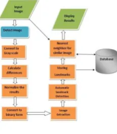
The aim of the research is to automatically generate 15 landmarks and then employ a distance based indexing method based on nearest neighbor to overcome this problem. Increasing the number of land marks from 13 to 15 facilitate in retrieving accurate and extensive searching. This is done by developing and employing a process of measuring distances between 15 facial points, generated automatically through a base line algorithm. The first phase is the face detection and recognition process, where an image will be taken as an input. Once a side view face image is identified it will be registered by automatically labeling 15 landmarks including 2 on ear. Then the distance between all 15 points is being calculatedusing pixels. Up to this point the face detection program plays its role. After all the distances are calculated between the landmarks highlighted, the information is stored in a database. In the second phase an image is being searched by nearest neighbor searching scheme. An image is being searched using these calculated registered land marks. After that the matching process starts where the calculated registered land marks of an image are being matched one by one in a sequence along with all the other side view face images stored in the database. If matching is successful then the result will be displayed showing all the similar face images.
Fig.2. Image Recognition Module
extraction using a baseline algorithm and along with nearest neighbor searching scheme. These steps are explained in detail as follows.
Step 1 : Face Detection
Converts a coloured input image to gray scale image as shown in Fig 3 by using the formula (1).
GRAY(i,j) = (IMAGE(i,j).Red + IMAGE(i,j).Green + IMAGE(i,j).blue )/3 (1)
Fig. 3(a). Colored image
Fig. 3(b). Extracted Gray Scale image
Step 2: Calculating Value differences
The next step is to calculate the difference between value of Red component from the value of Gray as shown in Fig 4 by using the formula (2):
Diff(i,j) = IMAGE(i,j).Red – GRAY(i,j) (2)
Fig.4. Calculated difference between Red and Gray component
Step 3: Normalize the result
Once the difference between the two components is computed the result is normalized to be from 0 to 255 as shown in the Fig 5. The normalization formula (3) is as follows:
newMin Min
Max
newMin newMax
Min I
In
( ) (3)
Fig.5. Normalized Result
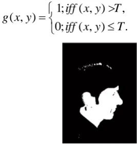
Step 4: Converting the image into binary form
Now we perform global threshold in order to convert the image into binary form as shown in the Fig 6. The conversion formula (4) is as follows:
.
)
,
(
;
0
,
)
,
(
;
1
)
,
(
T
y
x
iff
T
y
x
iff
y
x
g
(4)Fig.6. Converting image into binary
Step 5: Extraction of connected components
largest component. These connected components form an array whose elements are background values, in each connected component aforeground value also resides, as shown in Fig 7.
Fig.7. Extracting connected components
Step 6: Automatic Landmark detection
In this step the maximum x position of white pixels in each row are detected. Land marks are applied on exact position by using pixels.
Step 7: Storing landmark position in Array
Storing the position of each landmark that is automatically being placed in an array represented by a graph as shown in the Fig 8.
Fig.8. Graphical display of Array
Step 8: Nasal marking and Edge Detection for face image
Edge detection and maximizing the value for whole rows as a nose, shown in the Fig 9 by using the formula (5).
Ii
x
erf
Ii
Ir
x
f
)
1
)
2
(
(
2
)
(
(5)Fig.9. Automatic landmark placement on nose
As can be seen this phase is most critical as it initiates the automatic land marking process by identifying the nasal point.
Step 9: Height density search
The highest density area is found starting from the nose and going back to the ear as shown in Fig 10.
Fig.10. Highest density search
Step 10: Slope calculation on the graph
Next we calculate the slope between each point on the graph, the point when the slope is different from its previous slope state, depicted as a landmark, see Fig 11 (a) and Fig 11 (b).
Fig.11(a). Slope different states
Fig.11(b). 15 automatic landmarks
Step 11: Similar pictures search using nearest neighbor
Next we propose a nearest neighbor search algorithm which is a distance based indexing method. The number of points are positioned almost evenly and given a query point. This method often equal or exceed in accuracy much more complicated classification methods. The distances between facial features to search for the nearest feature is being employed [8]. We have used a simple design to classify nearest-neighbor
an image are being matched one by one in a sequence along with all the other side view face images stored in the database. On a given query image as shown in Fig 12 (a), if matching is successful then the result will be displayed showing all the similar faceimages as shown in Fig 12 (b), Fig 12 (c) and Fig 12 (d).
Fig.12(a). Input image
Fig.12(b). Output image 1
Fig.12(c). Output image 2
Fig.12(d). Output image 3
By using the proposed base line algorithm along with the nearest neighbor method a query search image, can retrieve and display multiple matching images from the database.
III. RESULTS
The proposed algorithm was tested on two fronts: speed of image retrieval and accuracy of image rertrival. Two tests were conducted in this regard, speed test and accuracy test. The results of both the tests are discussed below.
The proposed algorithm was tested on two fronts: speed of image retrieval and accuracy of image rertrival. Two tests were conducted in this regard, speed test and accuracy test. The results of both the tests are discussed below.
Speed Test (15 manual landmarks vs 15 automatic landmarks)
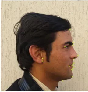
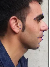
Speed test was carried to determine the time consumed to manually label 15 landmarks as shown in Fig 13 (a) and automatically labelling 15 landmarks on a side pose image as shown in Fig 13 (b). The comparison graph is also shown in Fig 14.
Fig.13(a). 15 Manually labeled landmarks
Fig.13(b). 15 Automatically labeled landmarks
Speed performance
Fig.14. Bar graph view of time difference
second and 97 mili seconds where as manual landmarking took 13 seconds and 27 mili seconds to label landmarks on a given image and as shown in table 1.
TABLE 1. 15 Manual vs 15 automatic labeled landmarks
Data 15 Manually
Labeled Landmark Time in seconds
15 Automatically Labeled Landmarks
Time in seconds
Difference
Input image
13s 27 ms 1s 97 ms 11s 3ms
Speed test (13 manual landmarks vs 15 automatic landmark)
Speed test was carried to determine the time consumed to maunally label 13 landmarks as shown in Fig 15 (a) and autoatically labelling 15 landmarks on a side pose image as shown in Fig 15 (b). The comparison graph is also shown in Fig 16.
Fig.15(a). 13 Manually labeled landmarks
Fig.15(b). 15 Automatically labeled landmarks
Speed performance
Fig.16. Bar graph view of time difference between 13 manual vs 15 automatically labeled landmarks.
The Fig 16 shows the total time taken to labe1 13 manual landmarks and 15 automatic landmarks. Automatic landmarking took merely 1 second and 94 mili seconds where as manual landmarking took 10 seconds and 24 mili seconds to label landmarks on a given image.
Total time taken in manually labeling 13 landmark points on a random side faceimage (measuring 1066 x800 pixels) using microsoft paint (10 seconds 24 milliseconds) and the total time taken in automatically labeling 15 landmark points on a random side face image using the matlab application (1 second 94 milliseconds) as shown in the Table 2.
TABLE 2. 13 manual vs 15 automatic labeled
landmarks Data 13 Manually Labeled Landmark Time in seconds
15 Automatically Labeled Landmarks Time in seconds
Difference
Input image 10s 24 ms 1s 94 ms 8s 3ms
Accuracy Test
Using a data set of 50 persons, a comparison of image retrieval was made between 13 automatically labeled landmarks and 15 automatically labeled landmarks. The images range in size from 4182x3096, 2666x2000, 2266x1700, 1999x1500, 1732x1300, 1466x1100, 1332x1000, 1066x800, 800x600, 666x500 and 399x300 pixels. The results are summarized in Fig 17. While in many cases the results appear to be the same, there are instances where using 15 landmarks, we were able to get more accurate image retieval results.
Fig. 17. line graph view of accuracy comparison between 13 and 15 automatic landmarks
The results of 50 dataset that were automatically labeled landmarked and then retrieved from database are summarized in the Table 3.
Data Set 113 Landmarks % results
15 Landmarks % results
1 100 75
2 50 50
3 75 100
4 100 100
5 50 75
6 100 75
7 50 50
8 9 10 11 12 13 14 15 16 17 18 19 20 21 22 23 24 25 26 27 28 29 30 31 32 33 34 35 36 37 38 39 40 41 42 43 44 45 46 47 48 49 50 _____________ 100 50 75 50 100 100 75 100 100 100 100 50 50 75 50 50 100 50 100 100 100 25 100 50 50 25 100 50 75 50 100 50 50 100 100 75 50 100 100 75 100 100 100 _______________ 100 50 75 75 75 100 75 100 100 100 100 75 50 75 75 75 75 75 100 100 100 25 75 75 75 50 100 75 75 75 100 100 50 50 75 100 100 75 100 100 100 100 100 _______________ Total 3850 4075
Fig.18. Accuracy result- Bar graph
The bar graph in Fig 18 shows the accuracy comparison between 13 and 15 automatic landmarks. Generalizing the results we can conclude that using 15 landmarks generate 4.5% more accurate results than 13 landmarks for image retieval as shown in the above Fig.
IV. CHALLANGES
Although the research has reached its aims some limitations of the study have been observed. These limitations become apparent during the course of the study. Natural facial features like thick moustache and beard constrain the accurate recognition of images. The algorithm is quick to recognize faces without substantial facial hair but does not give accurate results for faces having beard and moustache. Therefore, to generalize the results, the data sample included only those facial images which had no beards and moustache. There also lies further room for improving the algorithm to work with the background conditions such as light and texture. Dark background lighting constraints the results of the study.
Faces inclined due to extreme angles also constitute a short coming of the study. Finally, accessories such as spectacles and sun glasses fail to align the automatic landmarks accurately in the proposed algorithm.
V. CONCLUSION
An extensive method for recognizing side view facial images has been proposed. Many researchers have reported different techniques but all having some limitations. In order to minimizes computation time while achieving high detection accuracy, an approach is used to construct a face detection system which is much faster than any previous approach. By employing 2 new landmarks on ear lobes bringing to a total of 15 landmarks on facial features we broaden the range of recognition. Moreover as the landmarks are generated automatically and not manually, the response time is much lower and accurate. Coupled with the nearest neighbor approach, this novel algorithm is very efficient to overcome the challenges posed by side view face recognition. After repetitive tests it can safely be concluded that the proposed system can achieve 81.5% recognition accuracy rate whereas 13 automatic landmarks can achieve 77 %. Specifically the experimental results conclude that the 15 automatically generated landmark provides an effective mean towards pose-invariant face recognition.
VI. FUTURE WORK
The algorithm proposed is not absolute. In the future we aim to work on the following areas of the research to further improve accuracy results:
1. Improving the background conditions such as light and textured backgrounds.
2. Facial features like thick moustache and beard which constrain the recognition of images.
3. Various angles on which the face may be inclined.
REFERENCES
[1]. D. Hefenbrock, J. Oberg, N. T. N. Thanh, R. Kastner, S. B. Baden, " Accelerating Viola-Jones Annual International Symposium on Field-Programmable Custom Computing Mac pages 11-18. Face Detection to FPGA- Level using GPUs", FCCM '10 Proceedings of the 2010 18th IEEE.
[2]. P.Greeshma1, K. P. Rao, "Efficient Retrieval of Face Image from Large Scale database using spare coding and reranking", International Journal of Science and Research, volume 3 issue 9, september 2014.
[3]. M. Lew, N. Sebe, C. Djeraba and R. Jain, "Content-based Multimedia Information Retrieval", State of the Art and Challenges, Transactions on Multimedia Computing, Communications, and Applications, Volume 2 Issue 1, February 2006
[4]. P. S. Luuk, J. S. Raymond, N. J. Veldhuis, "Side-View Face Recognition", 32nd Symposium on Information Theory in the Benelux, WIC 2011, 10-11 May 2011, Brussels, Belgium (pp. 305-312).
[5]. R. Kleihorst, H. Broers, A. Abbo, H. Ebrahimmalek, H. Fatemi, H. Corporaal and P. Jonker," An Simd-Vliw Smart Camera Architecture For Real-Time Face Recognition", STW, Technology Foundation, 2003. - ISBN 90-73461-39-1. - p. 114
[6]. T. Ahonen, A. Hadid and Matti, "Face Recognition with Local Binary Patterns", Springer Berlin Heidelberg, Volume 3021, pp 469-481, 2004.
[7]. H. Haider, M. S. H. Khiyal, "Side-View Face Recongnition Using Enhanced Landmarks", Lambert Academy Publishing, Germany, Nov 2016. -ISBN: 978-3-330-00545-7.