Empiric On The Relationship Between Pollutant Emissions, Renewable Energy Consumption, And Economic Growth: Evidence From Sub- Saharan African Countries

2888

Empiric On The Relationship Between Pollutant

Emissions, Renewable Energy Consumption,

And Economic Growth: Evidence From Sub-

Saharan African Countries

Ali Umar Ahmad,Ibrahim Mohammed Adamu, Inuwa Mukhtar Ahmad, Suraya Ismail, Ibrahim Sambo Farouq, Aminu Hassan Jakada, Aminu Muhammad Fagge, Umar Abdul'Aziz Muhammad, Ahmad Tijjani Abdullahi, Umar Aliyu

Mustapha, Ismail Aliyu Danmaraya, Garba Ibrahim, Uzairu Muhammad Gwadbe

Abstract: This study offers an empirical analysis assessing the relationship between pollutant emission, renewable energy, interaction term, and economic growth when allowing for known breaks (recent energy crisis) based on a dataset of SSA countries spanning the years from 1970-2017 by using recently developed heterogeneous panel techniques. The study adopts a cross-section dependence test, unit root test; Levin-Lin-Chu, Im-Pesaran, Madalla and Wu, CIPS and the cointegration test; Westerlund and Edgerton, 2008 cointegration test which allows the structural breaks, Larsson, et al. 2001 cointegration test, and Wald test and Dumitrescu and Hurlin heterogeneous panel Granger causality test. The results of both the Larsson et al. 2001 cointegration test and Westerlund cointegration and Edgerton 2008 analysis reveal that the cointegration relationship between the variables exists. Moreover, the result shows that long-run and short-run coefficient for pollutant emission and recent energy crisis are negative and significant at 1%, while, the coefficients for the renewable energy and interaction (RXP) is positive and statistically significant. The Panel Dumitrescu and Hurlin heterogeneous causality reveal bidirectional relationship running from pollutant emission to economic growth, renewable energy to economic growth. In conclusion, the study recommends that cleaner technologies should be employed to optimize the benefits of wood bio mass as a renewable source of energy while minimizing its adverse effects; the share of other renewable energy components such as solar, wind and geothermal should be increased in the renewable energy mix of the sub-region of SSA, and more significant commitment to achieving sustainable renewable energy by SSA authorities is needed.

Index Terms: Pollutant Emissions, Renewable Energy, Consumption, Economic Growth, Westerlund. ——————————  ——————————

1 INTRODUCTION

There are quite several factors that determined the socio-economic welfare of a country, with the production of different products and services suitable for accommodating the needs of people as the primary factor. The ability of an economy in the production of goods and services relies on the quality and quantity of the available productive inputs, and these include land, capital, and labor. The number of energy use is said to be among other factors the most vital determinant of the economy‘s produce [1]. Therefore, economic development and growth mostly perceived as a significant contributed source of attaining improved persons, the wealth of the economy and enhanced prosperity. This all relies on the elaboration of capabilities of the country to make available production of goods and services derived by productive inputs expansion, which involves energy means and used energy. The focal point of recent globalization against the pressing effort to alleviate emissions to a Green House Gases (mostly initiated to be in charge of changes in climate and to attend its unwanted consequences) brought about tremendous debates across various organizations, academicians and institutions from developing and developed nations based on its likely implications [53].

Efforts being put globally to mitigate the undesirable change in climate led to the innovation and implementation at regional, national and international state. More notably, the Kyoto Protocol (1997), which refers to a treaty of international developed to alleviate emissions in reducing global warming. Economies that authorized the protocol promised that beginning in 2005; greenhouse emissions will reduce to 5% in 1990 levels. As the agreement at that time was a pledge, it barely provided a dent in several greenhouse gasses that were emitted. Even though a new essential step developed is the by the United Nations Framework Convention (UNFC) on Climate Change. This was signed on the 4th of November 2016 and ratified by economies numbering 147 for now. The agreement is to alleviate the global greenhouse emissions to achieve a temperature increase beneath 2°C [81]. Nonetheless, the use of energy as the primary energy source, particularly fossil fuels, has many adverse effects on the environment. Non-renewable energy consumption is a significant contributor to stationary Green House gas (GHG) emissions. Greenhouse gases are potentially critical to keeping the temperature of the earth warm. Whereas extra Greenhouse Gases, however, caused by activities of human capital, increasing heat absorption and global warming. Global warming is one of the biggest challenges facing policymakers at all levels, from global and international to national, regional and local. Global climate change threatens to disrupt society's well-being, undermine economic development and alter the natural environment, making it one of this century's key policy concerns. This problem requires a move from reliance on traditional non-renewable energy sources whose use contributes to GHG emissions causing climate change to a new focus on renewable energy sources such as solar photovoltaic energy, wind and other forms of renewable

___________________________________

 Author 1Ali Umar Ahmad, [email protected]

• Co-Authors 2Ibrahim Mohammed Adamu, 3Inuwa Mukhtar Ahmad, 4Suraya Ismail, 5Ibrahim Sambo Farouq, 6Aminu Hassan Jakada, 7Aminu Muhammad Fagge, 8Umar Abdul'Aziz Muhammad, 9Ahmad Tijjani Abdullahi, 10Umar Aliyu Mustapha, 11Ismail Aliyu Danmaraya, 12Garba Ibrahim, 13Uzairu Muhammad Gwadbe

2889 energy with little or no impact on climate change. Directive

2001/77/EC of the European Union defines renewable energy sources (RES) as non-fossil renewable energy sources that include wind, solar, geothermal, wave, tidal, hydropower, biomass, landfill gas, wastewater treatment plant gas and biogas [25]. The RES can not only reduce GHG emissions but also contribute to job creation and national energy supply protection. Given these submissions, it is imperative to investigate how the emissions of pollutants and renewable energy emitted from the use of fossil fuels can affect SSA economic growth. Different studies have been conducted to diagnose SSA countries ' growth and development problems, often using traditional growth models to identify the implications of certain fundamental variables, including capital formation, labor, human capital, and technology, for the region's growth and development. However, very few of these studies have identified energy use as a critical determinant of the region's economic growth [3]; [5]; [1] and [10]. Moreover, only fewer studies investigate the impact of energy on sub-Saharan Africa's economic growth, as they mostly focused on assessing the impact of renewable or non-renewable energy on the region's economic growth [2]. This study is, therefore, particularly interested in how renewable energy consumption and pollutants fit into the sub-Saharan African region's complex system of economic growth. The study aims to examine the effects of renewable energy consumption and emissions of pollutants as a CO2 proxy on SSA's economic growth to provide the SSA policymakers with political implications. This research overcomes literature gaps by using alternative modeling frameworks, longer samples than previous studies, recent advances in econometric techniques, and being the first to investigate the impact of renewable energy consumption along with pollutants on the region's economic growth.

2

EMPIRICAL

LITERATURE

Numerous academic papers have already explored the relationship between energy and economic growth over the past two centuries, often finding contradictory results and energy consumption. Nevertheless, it is argued that energy, along with other factors of production (such as labor and capital), is a necessary and sufficient output. Energy is, therefore, a prerequisite for economic and social growth that has become a "serious economic growth bottleneck" in theory [26]. From the other side, it is asserted that because energy prices are becoming a small fraction of GDP, they can never have a significant impact; hence, there is a "negative production energy effect" [20]. While strong linkages and causality among economic growth and energy consumption are vivid economic facts, economic growth causality and energy consumption are not adequately illustrated. The overall outcome changes accordingly with some studies that claim causality ranges from energy consumption to economic growth, whereas others say the reverse, even though most of the studies show bidirectional causality. While methodological differences explaining the varying results derived from these studies, similar methods implemented to data produced contradictory results for various countries, and it can, therefore, be seen that empirical studies examining the effect of energy on economic growth were generally inconsistent. Studies on the relationship between economic growth to energy introduced earlier bi-variate models for member countries and the results of time series. In initial researches,

2890

3 METHODOLOGY

3.1 Model Specification and Data

This research goes with the neo-classical improved Solow growth model, which Mankiw, Romer, and Weil (1992) first proved on the eve of the panel information system for Islam (1995). It takes into consideration the below growth model.

Where, stands for the production result, as capital refer to the labour force; whereas, is the efficiency and technological changes, individual economies, and time interval are given respectively as i and t. [76], [8], [75] and [54] to mention but few. It also will include in the model the renewable energy consumption and carbon emissions to analyze their effects on economic growth.

Where shows that gross domestic product per capita growth, depicts the renewable energy consumption, stands as the pollutant emission, shows the moderating role of these variables in the

model and It is

the error term. stands for the time interval in the study, and shows the individual countries. Furthermore, equation (3) shows the econometrics model:

Where stands as the natural logarithms of renewable energy consumption and carbon emission interaction term; denotes the dummy variable of the recent energy crisis of 2015.

This research uses annual panel data set from 1970 to 2017 to examine SSA economies ' renewable energy use and emission on economic growth. The timeline was implemented to take into account the significant events like the oil crisis of 1973, the global recession of the early 1980s, the oil shortage triggered by decline in demand by 1986s, the energy crisis of the 1970s, the stock market collapsed in the United States in 1987, the energy price rise following the 1990 invasion of Kuwait by Iraq, The world financial crises of 2007 and the 2015 recent Energy Crises. Renewable energy consumption and greenhouse gas emissions are the explanatory variables, whereas the growth per capita of real gross domestic product is seen as the explained variable. World Bank Development Indicators [83] will provide the information for this report. The study uses Panel econometrics methods to analyze the data.

3.2 Estimation Techniques

3.2.1 Cross-Section Dependence Test

Using panel data, it is an overall stage that there must be estimates for unit root and cross-sectional dependence. Else, it transforms out that regression is erroneous (Nelson and Plosser, 1982, [74]. The cross-sectional dependency measure evaluates the existence of cross-sectional dependency throughout the panel. For Pesaran (2004), it is the initial test that analyzes the series ' order of integration, and the main concern is to check the series ' cross-sectional dependence. It is also the first analysis test to determine suitable root unit tests. Cross-sectional independence indicated that error terms

are also not cross-correlated. Therefore, should the test show dependency and the researcher goes with independence methods, the result would end up being bias.

Where Denotes intercepts and slope, respectively, number of countries and t period for the study. For each and for all t, While they might be interrelated cross-sectionally. The dependence of Across could come variously. It can be as a result of unobserved standard components of The regressors could have lagged values of be either stationary or non-stationary. The CD test is as follows:

Where is the simple estimate of the Pair-wise correlation of the residuals.

is the ordinary least square estimate of in equation ( 6) above, it is defined as

3.3 Unit Root Test

The panel unit root test must be performed in the second phase to understand the stationarities' property of the parameters. Madalla and Wu, Levin-Lin-Chu (LL) test, Breitung test, Hadri test, ADF-Fisher Chi-square, CIPS test, Im-Pesaran-Shin (IPS) test, PP-Fisher Chi-square, Harris and Tzavakis panel data analysis are commonly used. This analysis, therefore, employs the test of Levin-Lin-Chu (LL), the test of Madalla and Wu, the test of Im-Pesaran-Shin (IPS), and the test of Cross-sectionally enhanced IPS (CIPS), depending on their various properties.

3.3.1 Levin-Lin-Chu Panel Unit Root Test

This is possible for moderately sized panel data. However, the segment has almost no power in serial connection testing, and it cannot be erased. The test is also carried out on the null hypothesis that perhaps the time series is non-stationary towards the alternative hypothesis that those series are stationary throughout the panel. LLC limits individual correlation, and it is not possible to remove correlation by dislodging cross-sectional averages.

Where are the deterministic variables,

is and .

3.3.2 Im-Pesaran Panel Unit Root Test

This is referred to as IPS. The unit root check of the IPS is often used to analyze the variables ' stationary properties. IPS has questioned and expanded Levin and Lin by allowing variability on the lagged explained variable coefficient and proposed reliable t-bar test statistics based on average Dickey-Fuller statistics across classes. The IPS test's null hypothesis can be calculated using the equation below:

Where the moments of

2891

3.3.3 Madalla and Wu Test

in your Madalla and Wu assessments are centered on the combined significance of various unit root. If the statistics for the test are continuous, the level of significance ( are independent and uniform (0,1) variables. This test uses combined p-values, which can be express as:

Where has a Distribution with degrees of freedom. Moreover, the below-standardized statistic was proposed by Choi (2006) proposed:

The hypothesis of cross-sectional independence, this statistic converges to a standard normal distribution [75].

3.4 Panel Cointegration Test

Throughout recent studies, the information literacy of the applied panel focused mainly on the study of co-integration to check the long-run relationship between the vectors. Co-integration tests like [41]; [82]; [30]; [28] have been established over the period. Pedroni, 1999; [52] co-integration tests supply contradictory and ineffective empirical outcomes due to their limited predictive power and presume that the variables must be assimilated at 1(I). In this study, the newly developed [82] and [41] of second-generation panel co-integration tests are used to examine whether the variables are co-integrated.

3.4.1 Westerlund and Edgerton (2008) Cointegration Test

This test is sufficiently versatile to allow for heteroskedastic and serially correlated error, cross-sectional, unknown structural breaks, and unit-specific time trends of the slope and intercept co-integration test. It also made it possible to detect the structural breaks at various dates. Also, under the null hypothesis, the test distribution was discovered to be healthy and free of nuisance criteria. The cointegration of this Panel has some benefits over the co-integration test of the first generation. The LM principle is used for testing purposes that, when evaluated at the vector of exact parameters below the null, the score vector has zero mean. The following pooled log-likelihood function is therefore considered by [80]:

The log-likelihood function on and then evaluating the resulting score at the restricted maximum likelihood estimates.

Let

, the score contribution for unit i will be

Where is a specific residual defined below, while and denotes the mean values of and . The score vector is proportional to the numerator of the least-squares estimate of in the regression

It implies that a cross-section segment I check of the null of no co-integration can be developed equally as a zero-slope constraint in equation (3.23), The least-square approximation of β I or its t-ratio can be checked. Thus, looking at the nature

of the log-likelihood function, a panel test of The cross-sectional sum of these statistics can be developed for each i. The factor it can be estimated as: in the presence of cross-sectional dependence.:

Where

The stands as the accumulated sum of the principal component estimates Of This refactoring makes the test robust to cross-sectional dependence derived by common determinants, while the test regression can, therefore, be augmented to as well lead to robustness to serial correlation. t=2,3, 4……T and This shows that the limited

maximum likelihood test of

and the remaining parameters estimates can be derived by OLS

regression of the equation

.

The proposed LM test of Westerlund and Edgerton (2008) are:

Where is the least square estimate of , and where R account for the lagged covariance of To be estimated in the variables. The null hypothesis for the panel tests is an alternative hypothesis is denotes group statistics that do no exploit the information concerning error correction.

3.4.2 Co-integration Test

Larsson technique enables on more than one vector of co-integration, but only one co-integrating vector is assumed by [63]. Eventually, while the co-integrating relationships are limited to each cross-section, the model's repository is unregulated, allowing for short-run dependence between the classes, the most attractive of these is the cross-sectional reliance on error terms. In order to begin the analysis. If integration has been found, the next step is to assess if the co-integrating coefficients are homogeneous or not. [42] consider co-integration testing on the assumption that: for …., N the null hypothesis is for …N against the alternative hypothesis that for a non-vanishing fraction of cross-section members. Furthermore, this test statistic in comparison to that of [35] and is known by a proportioned version of the cross-sectional average of the individual trace statistics. Indicates trace statistics for the null hypothesis of a k-dimensional co-integrating space for the unit I in which the superscript s suggests the materialist element requirements:

2892

by . and denote mean

and variance of the asymptotic trace statistics respectively found from a stochastic simulation (Johansen, 1995). For

the expressions and

converge to the limit of the expected value and variance of the trace statistic, respectively, equivalent to the case v deliberated. For each country in the panel, the null hypothesis, , is tested using the observed trace statistic. If the null hypothesis is rejected, then the null hypothesis, , is tested. This serial testing technique ends when the null hypothesis, is not rejected which determines the rank evaluation of r.

3.5 MG and PMG Estimates

Mean Group (MG) and Pooled mean group (PMG) techniques developed by [65] can assess the short-term and long-term coefficients. The PMG and MG estimators demonstrate both the reallocation of the long-run coefficients indicated by the homogeneity limitations and the team average used to obtain a method for the evaluated model's other short-run parameters and error correction coefficients. [65] categorized, for example, several factors that can be recognized as homogeneity in the long-term relationship covered by all groups; prevalent technologies, organizational development, and condition of arbitration. The MG and PMG estimators presumed homogeneous long-run parameters, providing a useful optimal choice between evaluating separate regressions, allowing all error variances and coefficients to differ across groups, and traditional specified-effect estimators, accepting all slope coefficients and error variances being the same. Taking into account the number of time series inferences available in each case, it will have the viable desired advantage in allowing the short-run dynamics to be decided for each nation. [65] reported that this is very important to distinguish between some instances of stationary and non-stationary regressors in order to push the exponential process of PMG estimators. In theory, identical algorithms can be used to measure the estimators of MG and PMG irrespective of whether the regressors are I (0) or I (1), the underlying asymptotic hypotheses are fundamentally disparate for these two cases, and their derivations require separate treatments. The PMG's primary benefit over the conventional specified-effect flexible model (DFE) is that it can allow the short-run dynamic configuration to vary from nation to nation. The lag order was first selected by the Schwarz Bayesian criterion (SBC) on the unrestricted model in each state, conditional to a maximum lag of 1. Nevertheless, there are several criteria for this methodology's accuracy, effectiveness, and credibility. First, the existence of a long-run connection between interest variables requires the coefficient on the term of error correction to also be harmful and not below -2. Secondly, A significant presumption for the continuity of the ARDL model is whether the independent variables are regarded as exogenous as well as the eventual residuals of the error correction model are not correlated in any way. Third, the comparable size of T and N is essential: in the average estimators, all should be huge to choose the diverse panel process to avoid the bias. [18] suggests that heterogeneity treatment is critical to understanding the cycle of development. Failure to meet these criteria will, therefore, produce various PMG estimates [77]. The Pooled Mean Group Model, including the long-term relationship among variables, may emulate the

methodology of [62]:

Where: is the first change operator, and Are the four variables selected in the study? The constant is , the short-run and long-run coefficients on the trends are:

respectively.

represents the maximum lag

length, are error terms.

3.6 Panel Causality Test

This analysis applied the Dumitrescu and Hurlin Heterogeneous Panel Granger Causality Estimates to establish the causal relationship here among candidate variables (G, R, P). In heterogeneous panel data models with defined coefficients, Granger (1969) developed the non-causality test. The increase in generic non-causality tests to panel data shows evaluating cross-sectional linear constraints on model coefficients in the context of a linear autoregressive data generation process. The use of cross-sectional data can extend the causality data sets from one variable provided to another. It is, of course, extremely possible in various economic issues that if a causal relationship happens for a nation or a person, it also exists for a different economy or community. Thus, there is no causal relationship for either of the panel's cross-sectional groups, the null hypothesis of Homogeneous Non-Causality (HNC). Conversely, however, there will be two categories of cross-section units: one characterized by x-to-y causal relationships and then another subgroup for which x-to-y causal relationship does not exist. The Granger various panel estimates of causality of Dumitrescu and Hurlin are:

Where Denotes constant in all the series, and signifies constant lag orders for all cross-sections of the panel. This allows As autoregressive coefficients and parameters of the slope to vary across the countries. The model is a fixed coefficient model and uses fixed special effects. The heterogeneous no-causality hypothesis the null

hypotheses: ( : ). The

value of F-statistics and p-value, which indicates whether or not to reject the null hypothesis, signifies the presence of causality or not.

4.

RESULT

AND

DISCUSSION

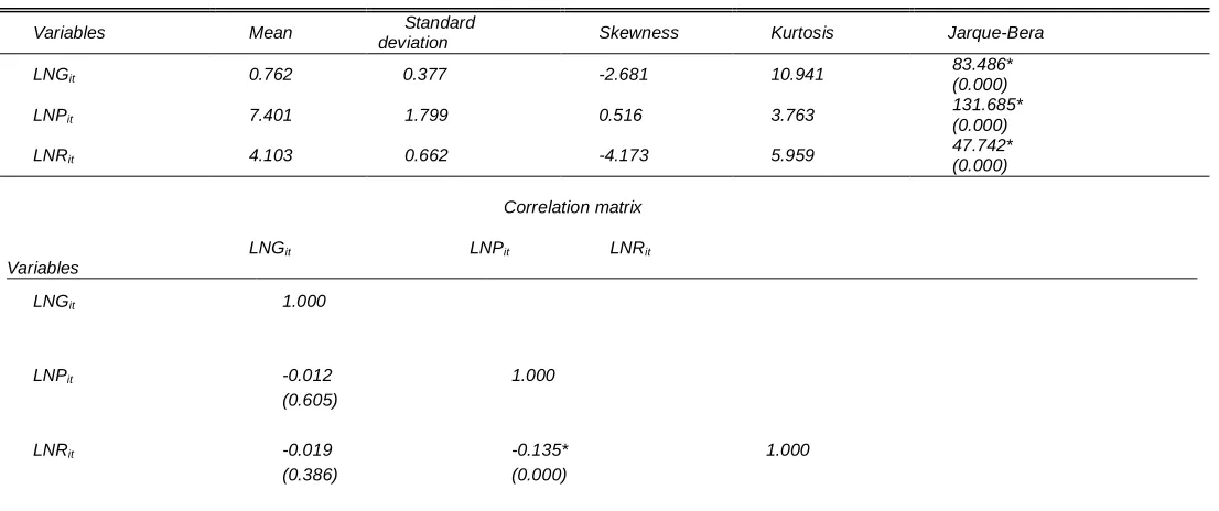
4.1 Descriptive Statistics and Correlation Analysis Results

2893 observation. Generally, if the Kurtosis and Skewness values

2894

Table 4.1 Summary Statistics

LNGit 1.000

LNPit -0.012 1.000

(0.605)

LNRit -0.019 -0.135* 1.000

(0.386) (0.000)

Notes: * and ** significant at 1 and 5% levels. Figures in () denote p-values

4.2 Cross-sectional Dependency Test Results

This study applied a testing instrument that works with the problem of cross-section dependence. In Table 4.2, the results of the CD tests concerning these correlations which show that P, G, and R are highly dependent on the economies. The values of probabilities in parenthesis depicts that the null hypothesis of independence is seriously rejected at 1% level of significance. This result underlines the already mentioned importance of taking into account cross-section dependence when analyzing the effect of P and R on G in the Sub-Saharan African Countries.

Table 4.2 Cross-sectional Dependence Tests

Variables Breush-Pagan

(LM) Test Pesaran’s CD Test

LNGit 7978.318*

(0.000)

3.649* (0.000)

LNPit 14189.96*

(0.000)

14.538* (0.000)

LNRit 14841.56*

(0.000)

75.022* (0.000)

Note: * and ** significant at 1 and 5% levels. Figures in ( ) denote p-values. Pesaran (2004) CD test takes cross-independence as the null, and the p-values are for the single test based on the normal distribution.

4.3 Unit root Test Results

The results from the CIPS test are documented in Table 4.4 that shows the findings of the unit root analysis of the factor components at a level for G, P, and R and found stationary at 1%, 5%, and 10% levels of significance. Therefore, the G, P, and R while at first difference gained stationary at 1% levels of significance. As such, the G, P, and R were stationary and integrated of the same order, at both I(0) and I(1).

Table 4.3 Panel Unit Root Test

Variables

Im et al. Madalla & Wu LLC CIPS

At level At first

different At level At the first diff At level

At first

different At level At first different

LNRGDPit -4.186* (0.298)

22.959* (0.000)

237.73* (0.000)

841.338* (0.000)

-5.224* (0.000)

-20.702* (0.000)

-3.528* (0.000)

-15.185* (0.000)

LNPit 0.4829*

(0.000)

-14.740* (0.000)

46.436* (0.000)

444.616* (0.000)

2.849* (0.002)

-10.242* (0.017)

0.606 (0.728)

-13.589* (0.017)

LNREit 5.016* _(0.000) -14.916* _(0.000) 68.038* _{(0.000) (0.000)} -13.589* 9.934* _(0.000) -10.888* _(0.000) 3.730* _(0.000) -11.694* _(0.000)

Notes: *, ** and *** Denotes rejection of the null hypothesis at 1% and 5% and 10% significance level.

4.4 Larsson Cointegration Test Result To identify the dynamic integration between pollutant

Variables Mean Standard

deviation Skewness Kurtosis Jarque-Bera

LNGit 0.762 0.377 -2.681 10.941 83.486* _(0.000)

LNPit 7.401 1.799 0.516 3.763 131.685*

(0.000)

LNRit 4.103 0.662 -4.173 5.959 47.742*

(0.000)

Variables

Correlation matrix

2895 emissions, renewable energy consumption, and economic

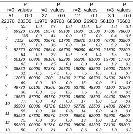
growth of SSA. This study uses [41] and [82]. For reliability at individual country level co-integration tests, the study employed the Likelihood-based co-integration test offered by [41] to allow for the possibility of multiple co-integrating vectors. The [41] co-integration result for SSA is reported in Table 4.5. Since the standard normal distribution, its 1%, 5%, and 10% critical values are 53.792, 47.181, and 43.964, respectively. Meanwhile, the results highlighted one co-integrating vector between P, R, and G at the 1% level of significance. Therefore, the panel rank test results reject the null hypothesis of no co-integration between the variables in SSA. Table 4.5 shows that the null of homogeneous co-integrating vectors is rejected as the test statistic, 63.37, exceeds the critical value of 43.964. Thus, this result is persistence with the previous studies of [67]; [73]; [13]; [22]; [20]. Which also recorded the co-integration relationship among P, R, and G in their studies. Nonetheless, The panel statistics ) and group means statistic rejects the null at a 1% level of significance. [58] given the same result that Pedroni‘s test statistics do not reject the null of no co-integration as structural breaks are included, they documented co-integration by way of the test proposed by [82]. A comparison with past studies, given exogenous break dates in the co-integration linkages between economic growth and energy consumption and economic growth, suggests that these results can be attested by [58] who showed structural breaks of the growth-energy consumption nexus for the SSA economies during the year 1980-1988.

Table 4.4 Larsson’s Heterogeneous Panel Co-integration

r=0 P

values r=1 P

values r=2 P

values r=3 P values 1 51. 22070 0.0 23300 27. 11970 0.0 98700 12. 68500 0.1 26900 3.1 56100 0.0 75600

2 55. 09920 0.0 09000 27. 10570 0.0 99100 11.0 1630 0.2 10500 1.8 07600 0.1 78800

3 136

.7112 0.0 00000 41. 02670 0.0 01700 17. 23670 0.0 27100 0.4 46700 0.5 03900

4 77. 82770 0.0 00000 36. 78540 0.0 06700 14. 95060 0.0 60300 5.2 21800 0.0 22300

5 64. 00120 0.0 00800 27. 86180 0.0 82200 7.8 55200 0.4 81000 1.5 19700 0.2 17700

6 ₀₈₈₅₀ 82. ₀₀₀₀₀ 0.0 ₉₇₃₇₀ 25. ₂₉₅₀₀ 0.1 ₁₈₀₀₀ 8.0 ₆₃₅₀₀ 0.4 ₁₆₀₀₀ 1.2 ₇₀₁₀₀ 0.2

7 31. 12060 0.6 60000 17.1 1700 0.6 31400 7.6 21700 0.5 06700 0.1 24600 0.7 24100

8 ₄₉₇₃₀ 69. ₀₀₁₀₀ 0.0 ₇₉₃₀₀ 30. ₃₈₃₀₀ 0.0 ₅₃₇₈₀ 15. ₄₉₃₀₀ 0.0 ₄₁₁₀₀ 7.1 ₀₇₅₀₀ 0.0

9 36. 18630 0.3 87000 16. 49170 0.6 77300 7.5 15500 0.5 18500 0.4 49400 0.5 02600

10 77. 09900 0.0 00000 42. 43720 0.0 01100 17. 62720 0.0 23500 5.2 14800 0.0 22400

11 55. 93950 0.0 07300 34. 92970 0.01 1700 14. 86510 0.0 62000 4.0 69900 0.0 43600

12 75. 59300 0.0 00000 35. 91780 0.0 08700 13. 98690 0.0 83300 1.2 78100 0.2 58300 13 50. 0.0 21. 0.3 8.6 0.3 1.3 0.2

27930 29100 72240 14200 97900 94100 31700 48500

14 69. 93570 0.0 00100 40. 46510 0.0 02100 17. 63500 0.0 23500 5.7 62100 0.0 16400

15 57. 93320 0.0 04300 31. 63400 0.0 30400 13. 25900 0.1 05600 1.9 48700 0.1 62700

16 55. 61230 0.0 07900 23. 38020 0.2 27900 7.6 46200 0.5 04000 2.5 55600 0.1 09900

17 44. 52970 0.0 99300 20. 73080 0.3 74600 7.6 64300 0.5 02000 0.1 78500 0.6 72700

18 55. 92350 0.0 07300 21. 92110 0.3 02900 3.7 86400 0.9 20000 0.3 54500 0.5 51600

19 84. 70220 0.0 00000 41. 43070 0.0 01500 17. 27140 0.0 26700 3.5 72100 0.0 58800

20 73. 41090 0.0 00000 32. 24880 0.0 25600 11.5 6910 0.1 78800 0.7 76900 0.3 78100

21 ₅₁₈₇₀ 50. ₂₇₅₀₀ 0.0 ₃₅₀₃₀ 24. ₈₆₀₀₀ 0.1 ₈₅₇₀₀ 5.3 ₆₆₆₀₀ 0.7₇₅₄₀₀ 0.4 ₉₀₅₀₀ 0.4

22 72. 49020 0.0 00100 40. 55840 0.0 02000 12. 81270 0.1 21900 4.4 10300 0.0 35700

23 ₉₇₇₆₀ 69. ₀₀₁₀₀ 0.0 ₄₇₉₈₀ 34. ₁₃₄₀₀ 0.0 ₃₃₈₇₀ 13. ₀₃₀₀₀ 0.1₉₄₀₀₀ 5.7 ₁₆₁₀₀ 0.0

24 77. 53420 0.0 00000 18. 94250 0.4 97000 9.6 65100 0.3 07400 1.5 78500 0.2 09000

25 71. 21680 0.0 00100 31. 99580 0.0 27500 16. 20280 0.0 39100 4.2 73000 0.0 38700

26 ₁₉₄₄₀ 56. ₀₆₈₀₀ 0.0 ₉₂₄₁₀ 33. ₁₅₈₀₀ 0.0 ₀₆₃₆₀ 15. ₅₈₀₀₀ 0.0₆₁₃₀₀ 4.8 ₂₇₅₀₀ 0.0

27 44. 54970 0.0 98900 25. 72500 0.1 37200 11.6 0080 0.1 77100 0.4 16700 0.5 18600

28 53.1 1870 0.0 14800 21. 78310 0.3 10700 9.9 28000 0.2 86300 1.4 22800 0.2 32900

29 46. 45950 0.0 67200 24. 60370 0.1 76100 9.4 91000 0.3 21900 2.1 84400 0.1 39400

30 73. 14930 0.0 00000 39. 92070 0.0 02500 19. 49010 0.01 1800 2.3 96400 0.1 21600

31 52. 52440 0.0 17100 25. 65460 0.1 39300 10. 57500 0.2 39000 4.6 09600 0.0 31800

32 121 .4187 0.0 00000 34. 85430 0.0 12000 11.4 4930 0.1 85300 0.7 45900 0.3 87800

33 62. 16450 0.0 01300 31. 10660 0.0 35100 10. 88670 0.2 18500 1.9 05200 0.1 67500

34 85. 37760 0.0 00000 29. 51360 0.0 53900 3.4 05600 0.9 45500 0.0 39500 0.8 42400

35 52. 82610 0.0 15900 21. 23030 0.3 43500 9.8 01000 0.2 96400 1.4 10700 0.2 34900

36 58. 53410 0.0 03600 31. 42050 0.0 32200 12. 87290 0.11 9600 4.5 22400 0.0 33400

37 54. 18950 0.01 1300 26. 10370 0.1 25600 8.7 05300 0.3 93400 0.5 25600 0.4 68500

38 32. 57500 0.5 80400 13. 73800 0.8 55000 6.9 56900 0.5 82700 0.7 30100 0.3 92800

39 57. 48980 0.0 04800 22. 94910 0.2 48600 7.5 92100 0.5 10000 1.6 32900 0.2 01300

40 38. 17290 0.2 94500 19. 90670 0.4 29200 7.4 24700 0.5 28800 1.4 08900 0.2 35200 LR_ NT 63.

37* _

28.

75 _

11.2

3 _

2.3

4 _

LR_ TEST

33.

51 _

17.

54 _

10.

05 _

5.1

0 _

E(Z _k)

27.7

3 _

14.9

6 _ 6.07 _ 1.14 _

Var( Z_k)

45.2

6 _

24.7

3 _

10.5

4 _ 2.21 _

N 40. 00 40. 00 40. 00 40. 00

Table 4.2 Summary Results of Heterogeneous

Co-integration Tests

Without trend

With trend

Test type Dependent Variable: LNRGDPit

p-2896

value value

Westerlund _{Gt -3.163* 0.000 -4.803* 0.000}

Ga -12.965** 0.036 -12.965* 0.000

Pt -16.149* 0.000 -16.149* 0.000

Pa

-32.570* 0.000 -32.570* 0.000

Note: * and ** denote rejection of the null hypothesis of no cointegration at 1 and 5% levels of significance, respectively, for Westerlund estimates. The AIC is used to choose the optimal lead and lag.

4.5 Diagnostic Tests and Hausman Test

The table presents the results of the diagnostics test showed that the hypothesized model statistically signifies the level of variance for the endogenous variables. The R2 values suggested that the pollutant emission, renewable energy consumption, recent energy crisis, and interaction term contribute about 71.9% and 67.2% of the economic growth of SSA. while the remaining 28.1% and 32.8%, might be due to other exogenous variables not captured in the model.

Meanwhile, the Hausman test is introduced to find the needed model from the two-panel data models [1]. The Hausman test result is shown in Table 4.7. It rejects the Mean Group model against the Pooled Mean Group. Hence, the null hypothesis of the Hausman test is accepted thereby validating the Mean Group model. Hence, the current study applied the Pooled Mean Group estimate to analyse the relationship between Pollutant emission, renewable energy consumption, interaction term, recent energy crisis and economic growth in SSA.

Table 4.7 Diagnostic Tests

0.719 0.717 1.743 2.38* (0.497)

0.977 (0.329)

0.723 (0.460)

Note that *, ** and *** denotes 1%, 5% and 10% significant levels respectively. AIC determines the optimal lag criteria. P-values are in parenthesis.

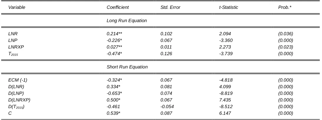
Table 4.8 Long-run and Short-run Estimates

Variable Coefficient Std. Error t-Statistic Prob.*

Long Run Equation

LNR 0.214** 0.102 2.094 (0.036)

LNP -0.226* 0.067 -3.360 (0.000)

LNRXP 0.027** 0.011 2.273 (0.023)

T2015 -0.474* 0.126 -3.739 (0.000)

Short Run Equation

ECM (-1) -0.324* 0.067 -4.818 (0.000)

D(LNR) 0.334* 0.081 4.099 (0.000)

D(LNP) -0.653* 0.074 -8.819 (0.000)

D(LNRXP) 0.500* 0.067 7.435 (0.000)

D(T2015) -0.461 -0.054 -8.512 (0.000)

C 0.539* 0.087 6.147 (0.000)

Table 4.8 shows the Long and Short-run findings of SSA economies. The bracket values represent t-statistics. The coefficient for long and short runs P-value depicts a negative sign at 1% concerning the recent energy crisis, while the coefficients for the interacting variable of R and P are positive and statistically significant. All the signs of the variables are following the theoretical predictions. In theory, the ectt-1 must be significant and negative. A higher coefficient means a stable short run. The coefficients of the ectt-1 of SSA are -0.324 (at 1% level of significance), which shows as a result of no changes in the independent variables, the speed of adjustment in respect to the deviation is corrected by 32.4% per annum which is faster. Moreover, the results depict that pollutant emission is harmful and significantly related to the economic growth in SSA in both long run and short run. A negative linkage between the pollutant emission and economic growth is in line with Burhan, [1], [78], [84], [51]. This follows

2897 industrial equipment exist. Conversely, the findings depict that

renewable energy used is positive and significantly linked to the economic growth in SSA in both the long and short run. A negative relationship among the renewable energy used and economic growth is in line with [13]; [25]; [59]; [61]; [87]. This records that in the long run 1% rise in renewable energy used will bring a 0.214 increase in economic growth, meanwhile in the short run 1% increase of renewable energy used will result in 0.334 rises in economic growth. This is because the majority of the renewable energy consumed in SSA emanates from wood sources, i.e., wood biomass [75]. Besides, the recent energy crisis result shows a negative and significant relationship concerning the economic growth in SSA both in the long and short run. This records that in the long run 1% rise in the recent energy crisis will bring 0.474 decreases in economic growth, while in the short run 1% increase of this energy crisis will result in 0.461 declines in economic growth. As globalization sets in, several issues have emanated among which include energy that got the attention of many researchers. However, the short and long-run effects of renewable energy used and pollutant emissions moderating the role of economic growth in the SSA is negative. Should the term become significant and positive, this would have been the pollutant emissions on economic growth goes up with renewable energy. Whereas, be negative and significant implies that the effect of pollutant emissions on economic growth reduces with renewable energy used. The result depicts that the interacting term is positive and significant. This means that the effect of pollutant emissions on economic growth is positive when moderated with renewable energy consumption in SSA.

Table 4.9 Granger Causality Results

LNRE LNRGDP

LNRE LNRGDP WHnc 2.803** 4.124*

(0.0453) (0.000)

LNP LNRGDP LNP LNRGDP

WHnc 7.462* 4.839*

(0.000) (0.000)

LNRE LNP LNRE LNP

WHnc 4.721* 3.786**

(0.000) (0.031)

The study uses the complex causality of Panel Dumitrescu and Hurlin Granger to study the causality of the dynamic panel. The complex causality of Panel Dumitrescu and Hurlin reveals a two-way relationship from pollutant emissions to economic growth, renewable energy to economic growth. Bidirectional causality from energy prices to economic growth is aligned with [16], [78], [84], [13], [14]; [59]; [61]; [87].

5. CONCLUSION

From the summary of the findings above, the finding shows that the type of renewable energy used in SSA slows rather than facilitates economic growth. This could be attributed to the fact that wood biomass; is the primary and accessible renewable energy in the sub-region, which is usually traditional and unclean. The use of this type of renewable energy is widespread in the sub-region, and its cost (adverse

effects) outweighs its benefits through indoor air pollution. Thus, marginally, SSA's use of renewables reduces production, as this study shows. However, Africa's energy sector is essential for its cycle of economic growth and development, but it is one of the world's most misunderstood energy systems. The growing importance of climate change issues and the need to find ways to mitigate greenhouse gases while maintaining sustainable economic growth has been at the forefront of the literature driven by energy production. The use of conventional fossil fuel energy sources such as petroleum, natural gas, and coal has been identified as the primary contributor to greenhouse gases leading to global warming.

6.0 Recommendations

This study examined data from the panel to explore the SSA nexus of pollutant emissions, renewable energy, and economic growth. First, since wood biomass is perhaps the most common origin of renewable energy in SSA, more great technologies are needed to optimize the use of wood biomass so that its benefits can be harnessed without adversely affecting the population's health. To accomplish this, a design of the renewable wood energy policy of the Member States of the European Union (EU) can be implemented into the renewable energy approaches of the Economic Community of West African States. West African countries can employ similar or sophisticated modern technologies used by EU countries. Second, in the sub region‘s renewable energy combination, the share of other renewable energy factors such as solar, wind and geothermal needs to be expanded. Thirdly, SSA countries need a stronger response to reaching green renewable energy. Though, the study recognizes both constant and constant trends as well as the long and short-run impact of known structural break (i.e., recent energy crisis) tests on co-integration. Thus, it would be quite useful to examine a structural break at the co-integrated point. In the presence of structural breaks, Gregory et al. (1996) investigate some of the issues associated with the co-integration test. They note that the existence of a structural break often creates false unit root in the system of co-integration, a small power to reject the null hypothesis of no co-integration emerges. That is, the existence of a structural break check makes it easy to assume this co-integration is not feasible. There are various types of tests at the co-integrated level for structural breaks. Although, the complex causality of Granger for the [41], [82], Pool Mean Group (PMG) and Panel Dumitrescu and Hurlin. The use of Lutkepohl tests, Hadri test, Breitung test, ADF-Fisher Chi-square, PP-ADF-Fisher Chi-square, Madalla and Wu test Bootstrap Causality, Generalized Momentum Model (GMM), Pedroni (Engle-Granger base) test for cointegration, McCoskey and Kao test for cointegration, and Fisher (Combined Johansen) test is recommended for further research.

6

REFERENCES

[1] W.-K. [1] Acheampong, A. O. (2018). Economic growth, CO2 emissions and energy consumption: What causes what and where? Energy Economics, 74, 677-692.

2898 [3] Adams, S., Klobodu, E. K. M., & Opoku, E. E. O.

(2016). Energy consumption, political regime and economic growth in sub-Saharan Africa. Energy Policy, 96, 36-44.

[4] Akarca, A. T. and Long, T. V. (1980). On the relationship between energy and GNP: A reexamination. Journal of Energy and Development, 5:326–331

[5] Ali, H. S., Law, S. H., Yusop, Z., & Chin, L. (2017). Dynamic implication of biomass energy consumption on economic growth in Sub-Saharan Africa: evidence from panel data analysis. GeoJournal, 82(3), 493-502. [6] Alshehry, A. S., & Belloumi, M. (2015). Energy consumption, carbon dioxide emissions and economic growth: The case of Saudi Arabia. renewable and Sustainable energy reviews, 41, 237-247.

[7] Ang, BW (2006). Monitoring changes in economy-wide energy efficiency: From energy-GDP ratio to composite efficiency index. Energy Policy, 34 (5), pp. 574-82.

[8] Ang, J. B. (2008). What are the mechanisms linking financial development and economic growth in Malaysia? Economic Modelling, 25(1), 38-53.

[9] Apergis, N., & Payne, J. E. (2010). Renewable energy consumption and economic growth: evidence from a panel of OECD countries. Energy policy, 38(1), 656-660.

[10] Appiah, M. O. (2018). Investigating the multivariate Granger causality between energy consumption, economic growth and CO2 emissions in Ghana. Energy Policy, 112, 198-208.

[11] Aslan, A. (2016). The causal relationship between biomass energy use and economic growth in the United States. Renewable and Sustainable Energy Reviews, 57, 362-366.

[12] Asongu, S., El Montasser, G., & Toumi, H. (2016). Testing the relationships between energy consumption, CO 2 emissions, and economic growth in 24 African countries: a panel ARDL approach. Environmental Science and Pollution Research, 23(7), 6563-6573.

[13] Bekun, F. V., Emir, F., & Sarkodie, S. A. (2019). Another look at the relationship between energy consumption, carbon dioxide emissions, and economic growth in South Africa. Science of the Total Environment, 655, 759-765.

[14] Bekun, F. V., Emir, F., & Sarkodie, S. A. (2019). Another look at the relationship between energy consumption, carbon dioxide emissions, and economic growth in South Africa. Science of the Total Environment, 655, 759-765.

[15] Boqiang Lin Mohamed Moubarakc (2014). Renewable energy consumption–Economic growth nexus for China; Elvevier; 40, 11-117

[16] Borhan, H., Ahmed, E. M., & Hitam, M. (2018). Co2, quality of life and economic growth in ASEAN 8. Journal of Asian Behavioural Studies, 3(6), 55-63. [17] Breitung J (2005) A parametric approach to the

estimation of cointegration vectors in panel data. Econ Rev 24(2):151–173

[18] Breusch, T. S. and Pagan, A. R. (1980) The Lagrange multiplier test and its applications to model specification in econometrics, Review of Economic

Studies, 47, 239–53.

[19] Chang Y (2002) Nonlinear IV unit root tests in panels with cross-sectional dependency. J Econ 110(2):261– 292

[20] Chen, S. W., Xie, Z., & Liao, Y. (2018). Energy consumption promotes economic growth or economic growth causes energy use in China? A panel data analysis. Empirical Economics, 55(3), 1019-1043. [21] Chen, Y., Wang, Z., & Zhong, Z. (2019). CO2

emissions, economic growth, renewable and non-renewable energy production and foreign trade in China. Renewable energy, 131, 208-216.

[22] Chen, Y., Zhao, J., Lai, Z., Wang, Z., & Xia, H. (2019). Exploring the effects of economic growth, and renewable and non-renewable energy consumption on China‘s CO2 emissions: Evidence from a regional panel analysis. Renewable energy, 140, 341-353. [23] Chontanawat, J, Hunt, LC & Pierse, R 2008. Does

energy consumption cause economic growth?: Evidence from a systematic study of over 100 countries. Journal of Policy Modeling, vol. 30, (2), 209-20.

[24] Dong, K., Hochman, G., Zhang, Y., Sun, R., Li, H., & Liao, H. (2018). CO2 emissions, economic and population growth, and renewable energy: Empirical evidence across regions. Energy Economics, 75, 180-192.

[25] Emir, F., & Bekun, F. V. (2019). Energy intensity, carbon emissions, renewable energy, and economic growth nexus: new insights from Romania. Energy & Environment, 30(3), 427-443.

[26] Ghali, K.H., El-Sakka, M.I.T. (2004) ―Energy use and output growth in Canada: A multivariate cointegration analysis‖, Energy Economics, 26, 225–238.

[27] Granger, C. W (1969) Investigating causal relations by econometric models and cross-spectral methods. Econometrica. Journal of Economics, 37(3):424–438 [28] Groen JJJ, Kleibergen F (2003) Likelihood-based

cointegration analysis in panels of vector errorcorrection models. J Bus Econ Stat 21(2): 295– 318

[29] Grossman, G. and Krueger, A. B. (1992). Environmental impacts of a north american free trade agreement. C.E.P.R. Discussion Papers, (644). [30] Hadri, K., (2000). Testing for stationarity in

heterogeneous panel application. Econometric Journal 3, 148–161.

[31] Hall, C. A. (2017). 11 Energy, economic growth and sustainability: an energy primer for the twenty-first century. Handbook on Growth and Sustainability, 232. [32] Harris, R.D.F. and E. Tzavalis, (1999) Inference for

unit roots in dynamic panels where the time dimension is fixed, Journal of Econometrics 91, 201-226.

[33] IEA (20017). World Energy Outlook.International Energy Agency. Paris, France

[34] IEA (2012). Energy Policies of IEA Countries Denmark 2011 Review. IEA Publications, Paris, Franc [35] Im, K.S., Pesaran, M.H., Shin, Y., (2003) Testing for

unit roots in heterogeneous panels. Journal of Econometrics 115 (3), 53–74.

2899 (1), 1127-1170.

[37] Johansen, S., (1988).Statistical analysis of cointegration vectors. Journal of Economic Dynamics and Control 12, 231–254.

[38] Kander, A., Malanima, P., and Warde, P. (2013). Power to People: Energy in Europe Over the Last Five Centuries. Unpublished

[39] Kedrosky, P. (2011). Cars vs cell phone embodied

energy. Online, Available at:

http://www.bloomberg.com/news/2011-06-15/cars-vs-cell-phone-embodiedenergy.html, [Accessed December-2018].

[40] Kraft, J. and Kraft, A. (1978).On the relationship between energy and GNP. Journal of Energy and Development, (3):401 – 403

[41] Larsson, R., Lyhagen, J., Löthgren, M., (2001). Likelihood-based cointegration tests in heterogeneous panels. Econometrics Journal 4, 109–142

[42] Lean, H. H., Mishra, V., & Smyth, R. (2015). The relevance of heteroskedas-ticity and structural breaks when testing for a random walk with high-frequency financial data: Evidence from ASEAN stock markets. The Handbook of High Frequency Trading, 59-73. [43] Lee, CC &Chien, MS 2010.Dynamic modelling of

energy consumption, capital stock, and real income in G-7 countries. Energy Economics, 32, (3), 56481. [44] Lee, J. W. (2013). The contribution of foreign direct

investment to clean energy use, carbon emissions and economic growth. Energy Policy, 55, 483-489. [45] Levin, A., Lin, C.F., Chu, C., (2002) Unit root tests in

panel data: asymptotic and finite-sample properties. Journal of Econometrics 108, 1–24.

[46] MaamarSebri and Ousama Ben-Salha (2014). On the causal dynamics between economic growth, renewable energy consumption, CO2 emissions and trade openness: Fresh evidence from BRICS countries. Elsevier; 39

[47] MacKay, D. J. C. (2009). Sustainable energy–without the hot air.UIT, Cambridge, England.

[48] Maddala, G.S., Wu, S.A., (1999) Comparative study of unit root tests with panel data and a new simple test. Oxford Bulletin of Economics and Statistics 108, 1– 24.

[49] Mahadevan, R &Asafu-Adjaye, J 2007. Energy consumption, economic growth and prices: A reassessment using panel VECM for developed and developing countries. Energy Policy, 35, (4), 2481-90. [50] Mankiw, N. G., Romer, D., and Weil, D. N., (1992) A contribution to the empirics of economic growth, National Bureau of Economic Research.

[51] Mardani, A., Streimikiene, D., Cavallaro, F., Loganathan, N., & Khoshnoudi, M. (2019). Carbon dioxide (CO2) emissions and economic growth: A systematic review of two decades of research from 1995 to 2017. Science of the total environment, 649, 31-49.

[52] McCoskey S, Kao C (1998) A residual-based test of the null of cointegration in panel data. Econ Rev 17(1):57–84

[53] McNulty, S., Weiner, S., Myers, J. M., Farahani, H., Fouladbash, L., Marshall, D., & Steele, R. F. (2015). Southeast regional climate hub assessment of climate change vulnerability and adaptation and mitigation

strategies. Agriculture Research Service, 2015, 1-61. [54] Menyah, K &Wolde-Rufael, Y (2010) ‗Energy

consumption, pollutant emissions and economic growth in South Africa‘, Energy Economics 32 (2), 2010.

[55] Menyah, K., &Wolde-Rufael, Y. (2010).CO 2 emissions, nuclear energy, renewable energy and economic growth in the US. Energy Policy, 38(6), 2911-2915.

[56] Moon, H. R. and Perron, B. (2004) Testing for a unit root in panels with dynamic factors, Journal of Econometrics, 122, 81–126.

[57] Moreau, V., & Vuille, F. (2018). Decoupling energy use and economic growth: Counter evidence from structural effects and embodied energy in trade. Applied Energy, 215, 54-62.

[58] Narayan, P 2005. The saving and investment nexus for China: evidence from cointegration tests. Applied Economics, 37, (17), 1979-90.

[59] Ozcan, B., & Ozturk, I. (2019). Renewable energy consumption-economic growth nexus in emerging countries: A bootstrap panel causality test. Renewable and Sustainable Energy Reviews, 104, 30-37.

[60] Pablo-Romero, M. D. P., & Sánchez-Braza, A. (2015). Productive energy use and economic growth: Energy, physical and human capital relationships. Energy Economics, 49, 420-429.

[61] Pao, H. T., & Chen, C. C. (2019). Decoupling strategies: CO2 emissions, energy resources, and economic growth in the Group of Twenty. Journal of cleaner production, 206, 907-919.

[62] Pedroni, P., (1999) Critical values for cointegration tests in heterogeneous panels with multiple regressors. Oxford Bulletin of Economics and Statistics 61, 653–670.

[63] Pedroni, P., (2004) Panel cointegration: asymptotic and finite sample properties of pooled time series tests with an application to the PPP hypothesis: new results. Econometric Theory 20, 597–627.

[64] Pesaran MH (2007) A simple panel unit root test in the presence of cross-section dependence. J Appl Econ 22(2):265–312

[65] Pesaran MH, Shin Y, Smith RJ. (1999) Bound testing approaches to the analysis of level relationship. J ApplEconom 16(3):289-326.

[66] Pesaran, M. H. (2004) General diagnostic test for cross section dependence in panels, Cambridge Working Papers in Economics, 0435, Faculty of Economics, University of Cambridge.

[67] Rasoulinezhad, E., & Saboori, B. (2018). Panel estimation for renewable and non-renewable energy consumption, economic growth, CO 2 emissions, the composite trade intensity, and financial openness of the commonwealth of independent states. Environmental Science and Pollution Research, 25(18), 17354-17370.

[68] Rodrik, D., Subramanian, A. and Trebbi, F. (2004) ―Institutions Rule: The Primacy of Institutions Over Geography and Integration in Economic Development, Journal of Economic Growth, 9, 131-65.

2900 Greece before and during the economic crisis and

their decoupling from economic growth. Renewable and Sustainable Energy Reviews, 76, 448-459. [70] Romer, P.M. (1986) ―Increasing returns and long-run

growth‖, Journal of Political Economy, 94(5), 1002-1037.

[71] Romer, P.M. (1990) ―Endogenous Technological Change‖, Journal of Political Economy, 98 (5), 71-102. [72] Saidi, K., &Hammami, S. (2015). Energy consumption and economic growth nexus: Empirical evidence from Tunisia. American Journal of Energy Research, 2(4), 81–89

[73] Salahuddin, M., Alam, K., Ozturk, I., & Sohag, K. (2018). The effects of electricity consumption, economic growth, financial development and foreign direct investment on CO2 emissions in Kuwait. Renewable and Sustainable Energy Reviews, 81, 2002-2010.

[74] Sbia, R., & Al Rousan, S. (2015). Does Financial Development Induce Economic Growth in UAE? The Role of Foreign Direct Investment and Capitalization. Working paper. University Library of Munich, Germany.

[75] Shahbaz, M., Khan, S., & Tahir, M. I. (2013). The dynamic links between energy consumption, economic growth, financial development and trade in China: fresh evidence from multivariate framework analysis. Energy economics, 40, 8-21.

[76] Sharma, R., &Bardhan, S. (2016). Finance growth nexus across Indian states: evidences from panel cointegration and causality tests. Economic Change and Restructuring, 1-20.

[77] Smil,V.(2010). Energy transitions: history, requirements, prospects. Praeger Publishers, Santa Barbara, California.

[78] Song, C., Liu, Q., Gu, S., & Wang, Q. (2018). The impact of China's urbanization on economic growth and pollutant emissions: An empirical study based on input-output analysis. Journal of cleaner production, 198, 1289-1301.

[79] Soytas, U., Sari, R., and Ewing, B. T. (2007). Energy consumption, income, and carbon emissions in the United States.Ecological Economics, 62(34):482 – 489

[80] Tugcu, C., Ozturk, I., & Aslan, A. (2012). Renewable and Non-Renewable Energy Consumption and Economic Growth Relationship Revisited: Evidence from G7 Countries. Energy Economics. 6 (2): 202-221 [81] United Nations Population Division (2014). World

Countries Population

[82] Westerlund, J. and D. L. Edgerton (2008).A simple test for cointegration in dependent panels with structural breaks. Oxford Bulletin of Economics and Statistics 70(5), 665–704.

[83] World Bank (2018) World Development indicators, World Bank, Washington, DC.(YemaneWolde-Rufael, 2005). Energy demand and economic growth: The African experience. 27, (8), 891-903

[84] Xie, R., Zhao, G., Zhu, B. Z., & Chevallier, J. (2018). Examining the factors affecting air pollution emission growth in China. Environmental Modeling & Assessment, 23(4), 389-400.

[85] Yu, E. and Hwang, B.-K. (1984). The relationship

between energy and GNP. further results. Energy Economics, 6(3):186–190

[86] Yu, E. S. H. and Jin, J. C. (1992). Co-integration tests of energy consumption, income, and employment. Resources and Energy, 14(3), 259–266