A Life Extend Approach Based on Priority Queue N Strategy for Wireless Sensor Network

(1)

1

A Life Extend Approach Based on Priority Queue N Strategy for Wireless Sensor Network

Jyun-Fan Ke, Wen-Ju Chen and Der-Chen Huang

Department of Computer Science and Engineering, National Chung Hsing University, Taiwan, R.O.C. [email protected]

Abstract

In this paper, we proposed a method on the tradeoff between packet transmission speed and battery life in wireless sensor networks (WSN). The data obtained by sensor nodes comprised various types of information with various levels of importance.A misjudgment of the priority of packets according to the importance of data may delay the transmission of important information. The energy consumed by sensor nodes varies according to system states. Therefore, this research used queuing theory and the birth-death process to build a mathematical model capable of quantifying various energy consumption parameters. MATLAB was used to calculate the distribution of system state probability for sensor nodes with two queues. Packet delay equation was then applied to obtain the expected values of delay time for packets of various priorities. We adjust various system parameters and observe how these changes influenced system state probability. Finally, we use different N values to obtain the minimal value of system energy consumption. Obtaining this value helps to overcome the energy hole problem (EHP), which in turn extends the lifespan of the overall WSN. Prioritizing packets can ensure the transmission of important data within a shorter time span. Experimental results show the energy consumption is reduced and important data can be transmitted with less packet delay time.

Keywords: WSN, EHP, Queuing Theory, Preemptive

Priority Queue, Ubiquitous Sensor Networks

1. Introduction

The sensor nodes have been popularly used in the application of wireless sensor network (WSN). Mike first introduces the ubiquitous computing concept in 1991. The concept has been extensively used to increase the convenience of human life. The sensor node is becoming one key device to consist of the intelligent ubiquitous computing network (USN) such as medical monitoring, surveillance and tracking systems [1, 2]. Most of the USN is to collect and relay information to coordinator for integrating as useful knowledge [3, 4]. Each sensor may provide several different kind of information with different priority and importance. To ensure the important information can be transmitted in real-time manner, we schedule the information with different sequence based on its priority. Meanwhile, the network disconnection problem becomes more important when the scale of ubiquitous sensor network is increased. Most of the network disconnection problem is induced from the power consumption issues. Thus, the real-time and power consumption [5, 6] issues become a critical topic while considering to extending the lifetime and availability of ubiquitous computing network.

The energy consumption of sensor node is larger if the sensor node is near the sink node. This result in the energy hole problem (EHP) may happen [7]. The USN cannot work normally due to the network disconnection. According to the report of [8], there is 90 % energy left when the lifetime of WSN is ended. This is because there is more data packets to be relayed through these coordinate sensor nodes such that the energy consumption of

coordinate sensor node is larger than other sensor node. First Come First Service (FCFS) has been adopted in most USN applications. However, if there are some emergency data to be transmitted, the scenario might not be working properly. To resolve the EHP [9, 10, 11] and packet transmission real-time issues, we proposed a method based on threshold and priority queue to deal with the energy consumption and real-time transmission. This paper is arranged as follows. The second section discusses the related researches. The system infrastructure, analysis method, power consumption and the packet delay time are discussed in the third section. Experimental results are discussed in the fourth section. The fifth section is the conclusion.

2. Related Works

In [12], the average power demand of USN in sleep mode is 30mW and 80mW in transmission mode. Many researches [13,14] focus on the extension of life cycle in sleep mode. If the collision is happened, there is more power consumption in system [15]. The queue module of M/M/1/K is discussed in [16,17,18,19] to reduce the collision. These researches use single queue to save data packet and a threshold N as a basis to access the radio channel. When the number of packets in queue exceeds N, it tries to seize the channel for packet transmission.

The USN has to transmit data packet smoothly with considering to saving more power. USN does not transfer or receive any packet when it is in sleep mode. It only checks whether the incoming data packet is related to itself or not. If it’s not in sleep mode when the related data packet is arrival, it is woken up from sleep mode [20, 21]. The process priority can be divided into non-preemptive priority and preemptive priority. Several researches [22,23,24,25] applied this approach on a queue structure buffer. The preemptive priority queue is favorable for higher priority packet by shortening the queuing time. In this paper, we proposed a method with dual queue priority structure to ensure the critical data packet can be handled in a more real-time manner with considering the extension of life cycle.

3. System Infrastructure

3.1 System Environment

In this research, we assume the transmission is in a half-duplex manner due to the concern of energy issue. Meanwhile, we set the queue size to be limited based on the realistic point of view. The system with four states, including Sleep State, Idle State, Busy State and Transmit State are also defined. The operation activities for each state can be shown in Figure 1. We define the priority level for each data queue to ensure critical information can be transmitted within a predicable period. To be more simplicity, we have illustrated a dual queue-based sensor node as an example. The high and low priority packets are named as n1 packet and n2 packet, separately. The high priority packet is stored in queue 1, and the low priority packet is in queue 2. The system is in sleep state at the initial phase of USN. There isno packet in the queue 1 and queue 2 at that time. The USN keeps stay at the sleep state

(2)

2 and assigns n1 and n2 packets respectively to the queue 1 and queue 2. After that, the USN is wakeup and enters into the idle state. In idle state, the sensor node keeps continuing to receive the data packets until the number of packets in queue 1 and queue 2 is identical to N. Then, the USN changes to busy state.

When in busy state, the sensor node starts to access the radio channel. In general, the queue size is limited. We assume the queue size is K. The receiving activity of queue 1 and queue 2 will be stopped completely if the number of receiving data packets in queue 1 and queue 2 is equal to K. We assume n1 packet has higher priority than n2 packet. For the case of queue 1 is full and queue 2 is not full, if there is any n1 packet arrived, the n1 packet will be dropped. In contrast, the n2 packet will be stored into the queue 2 buffer since the number of n2 packet in queue 2 is still less than K. If the sensor node access the radio channel successful at busy state, it enters into the transmit state and doesn’t receive any data packet. It transmits data packet in the queue until it is empty. The sensor node releases the access authority in case both queue 1 and queue 2 are empty. After that, it enters into the sleep state.

Server in sleep state (radio TX is off)

Server in idle state (radio TX is off) Receive a packet

Is queue 1 N-Policy

condition satisfied? No condition satisfied?Is queue 2 N-Policy

Server in busy state (competing for

channel )

Is the queue 1 empty? Competition success

Transmitting the queue 1's packet

No

Is the queue 2 empty? Yes

Transmitting the queue 2's packet

No Yes Server receive

packets Is the queue 1 or queue 2 fulled?

Drop p1 or p2 packet Yes No

p1、p2

collision

Server in transmitting state

(radio RX is off)

p1 p2

No Yes

Yes

Figure 1: System operation flow

3.2 System Power Consumption

Generally, the number of packets in queue and transmission activity will affect the power consumption of sensor node. The power consumption in one cycle is shown in Figure 2, where the x and y axis denote the time and power consumption respectively. In the beginning, the sensor node stay at the sleep state and there is no packet accepted in the queue. The state changes to idle state if any data packet arrived. The power required at this period is called setup energy. The sensor node continues to accept the data packet such that it requires more energy to keep the increased data packet. Once the number of data packets in queue is equal to N, the state changes to busy. The sensor

detects whether the radio channel is occupied by other nodes and gets the control authority of accessing radio channel. If the access is failed, it keeps staying at the idle state and continues to accept the data packet. These activities result in more energy needed to keep data packet in the queue. Otherwise, the state switches to transmit state to transmit data packet in the queue until it is empty. Then, the state is switched to sleep state.

Figure 2: System power consumption

At beginning, the state of USN is in sleep mode with no packet in memory buffer. When USN detects incoming packet, it is waked up and the system turned into idle state. USN receives the delivered packet when it’s in idle state. To hold the packet in buffer memory, the power supply for USN cannot be stopped. When the number of packets in buffer memory is up to threshold N, the system changes to busy mode. The USN antenna module detects whether the radio channel is occupied and tries to access the channel. If it is failed, the USN receives the packet during waiting time. Otherwise, the system changes to transmit mode and the USN starts to transfer the packet in buffer memory.

3.3 System State Transformation

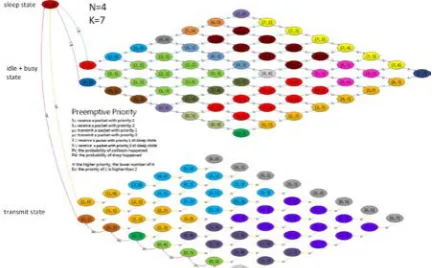
We adopted the birth-death graph technique to evaluate the probability for each state as shown in Figure 3. Each sensor node includes two queues (queue 1 and queue 2). The symbol (n1, n2) denotes the number of packets in the queue 1 and queue 2. For example, there is (0, 0) for the sleep state in the beginning, where both ‘0’ represent that there isn’t any data packet in the queue 1 and queue 2 at the start off phase. Similarly, the Ps, Pi, Pb, Ptand Pd represent

the probability of sleep, idle, busy, transmit and drop states, respectively. We assume the average data input rate follows the Poisson distribution, where λ'₁ and λ'₂ are data input rate in respect with n1 and n2 packets for the idle state. Similarly,

1

λ and

2

λ are used to denote the data input rate for the other states. The

1

µ and

2

µ are used to indicate the average service rate for the n1 and n2 packets, respectively.

(3)

3 packets until the number of packets in any of the buffer memory is reached to the buffer maxima size. After that, the income packet will be dropped because the buffer memory is full. The Pd indicates that the probability of dropping data if the queue is not available. The packet in queue will be transmitted with rate of µ₁ or µ₂ if the radio channel is available. The USN transfers all queue 1 and queue 2 packets following the priority in transmit mode.

Figure 3: System state transformation

3.4 Balance Formulation

To obtain the balance formula, we follow the method of induction. Based on the Figure 3, we derivate twenty-five general formulas by using graph with the case of N=4 and K=7, where N is the threshold value and K is themaxima size of buffer.

For the case 1 as Figure 4 (a) shows, the formula 1 shows the balance equation for the sleep state Ps(0,0), where the leave expectation value 𝑃𝑃𝑠𝑠(0, 0)�λ'₁+λ'2� is

equal to the incoming expectation value from transmit state

Pt(1, 0) or Pt(0, 1). The 𝑃𝑃_𝑡𝑡(1, 0) and 𝑃𝑃_𝑡𝑡(0, 1) will switch to 𝑃𝑃𝑠𝑠(0, 0) if the data packet is transmitted out from buffer memory with rate

1

µ or

2

µ .

𝑃𝑃𝑠𝑠(0, 0)�λ'1+λ'2� =𝑃𝑃𝑡𝑡(1, 0)µ1+𝑃𝑃𝑡𝑡(0, 1)µ2 ... (1)

In Figure 4 (b), the balance equation of cases 2 can be expressed as formulas 2 and 3. The input expectation value and output expectation value are identical for 𝑃𝑃𝑖𝑖(1, 0) and 𝑃𝑃𝑖𝑖(0, 1). The balance equation in Figure 4 (c) can be expressed as:

𝑃𝑃𝑖𝑖(3, 0)�λ1 +λ2� =𝑃𝑃𝑖𝑖(3−1, 0)λ1 ... (4)

2≤3≤4−1

,where the “3” and “3-1” can be replaced asn1 and n1-1, respectively for a general case as formula 4 shows. Similarly, the formula 5 can be obtained with the same method according to the Figure 4 (d). Again, the balance equation for the case 4 is: 𝑃𝑃𝑖𝑖(2, 2)�

1

λ +λ2� =

𝑃𝑃𝑖𝑖(2, 2−1)λ2+𝑃𝑃𝑖𝑖(2−1, 2)λ1, where n1 and n2 are

identical to 2 in Figure 4 (e). The general form can be written as formula 6.

𝑃𝑃𝑖𝑖(1, 0)�λ1 +λ2�=𝑃𝑃𝑠𝑠(0, 0)λ'1 ... (2)

𝑃𝑃𝑖𝑖(0, 1)�λ1 +λ2�=𝑃𝑃𝑠𝑠(0, 0)λ'2 ... (3)

𝑃𝑃𝑖𝑖�n1, 0� �λ1 +λ2�=𝑃𝑃𝑖𝑖�n1−1, 0�λ1 ... (4)

2≤ n1≤N−1

𝑃𝑃𝑖𝑖�0,n2� �λ1 +λ2�=𝑃𝑃𝑖𝑖�0,n2−1�λ2 ... (5)

2≤n2≤N−1

𝑃𝑃𝑖𝑖�n1, � �λ1 +λ2�=𝑃𝑃𝑖𝑖�n1,n2−1�λ2+𝑃𝑃𝑖𝑖�n1−1

,n2�λ1 ...(6)

1≤ n1≤N−1 & 1≤n2≤N−1

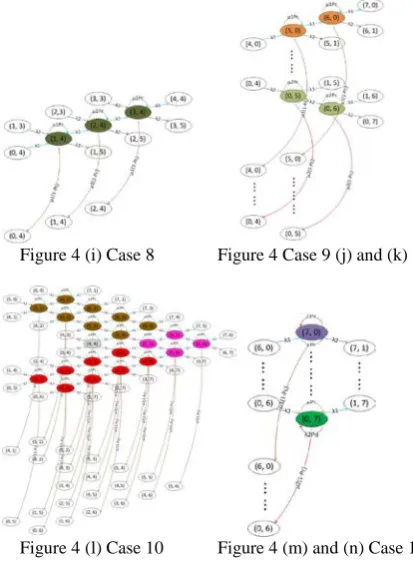
Figure 4 (a) Case 1 Figure 4 (b) Case 2

Figure 4 (c) Case 3 Figure 4 (d) Case 3

Figure 4 (a), (b), (c) and (d): System state transformed from sleep mode to idle mode

Figure 4 (e) Case 4: System state transformed from idle mode to busy mode

Formulas 7 to 18 are balance equation for the busy state. Its range involves the transition from 𝑃𝑃_𝑏𝑏(𝑁𝑁, 0) and 𝑃𝑃𝑏𝑏(0,𝑁𝑁) to 𝑃𝑃_𝑏𝑏(𝐾𝐾,𝐾𝐾). Based on the birth-death graph, we derivate the formulas 7 to 18 by using the same deductive method based on the Figure 4 (f) to (n). For example, in Figure 4 (l) of case 10, the balance equation is shown as: 𝑃𝑃𝑏𝑏(7, 2)�λ₂ + µ1(1− 𝑃𝑃𝑐𝑐)�=𝑃𝑃𝑏𝑏(7, 2−1)λ1 +𝑃𝑃𝑏𝑏(7−1,2)λ1

1≤2≤7−1.

In this case, the n2 and K is equal to 2 and 7, respectively. The general form can be shown as formula 16.

Figure 4(f) Case 5 Figure 4 (g) Case 6 Figure 4 (h) Case 7

The balance equations for the transmit state can be listed as formulas 20 to 25. For example, the case 12 in Figure 4 (o), its balance equation is:

𝑃𝑃𝑡𝑡(3,0)µ1 =𝑃𝑃𝑏𝑏(3 + 1, 0)µ1(1− 𝑃𝑃𝑐𝑐) +𝑃𝑃𝑡𝑡(3 + 1, 0)µ1

(4)

4 area, where n1 and n2 is equal to 3 and 0 respectively. The conditions for the purple and cyan areas are listed with respect to 1≤ ≤N−2 & N≤ n₂≤K and N−1≤

≤K−2 & N≤ n₂≤K. So, the n1 and n2 are located either in one of these conditions. Hence, the general form can be obtained as formula 20 shows.

Figure 4 (i) Case 8 Figure 4 Case 9 (j) and (k)

Figure 4 (l) Case 10 Figure 4 (m) and (n) Case 11

Figure 4 (f)~4 (n): System state transformed from busy mode to transmit mode

Figure 4 (o) Case 12: System transmit state

𝑃𝑃𝑏𝑏(𝑁𝑁, 0)�λ1 +λ2 + µ1(1− 𝑃𝑃𝑐𝑐)�=𝑃𝑃𝑖𝑖(𝑁𝑁 −1, 0)λ1 .... (7)

𝑃𝑃𝑏𝑏�𝑁𝑁,n2� �λ1 +λ2 + µ1(1− 𝑃𝑃𝑐𝑐)�=𝑃𝑃𝑖𝑖�𝑁𝑁 −1,n2�λ1

+𝑃𝑃𝑏𝑏�𝑁𝑁,n2−1�λ2 ... (8)

1≤n2≤N−1

𝑃𝑃𝑏𝑏(0,𝑁𝑁)�λ1 +λ2 + µ2(1− 𝑃𝑃𝑐𝑐)�=𝑃𝑃𝑖𝑖(0,𝑁𝑁 −1)λ2 .... (9)

𝑃𝑃𝑏𝑏�n1,𝑁𝑁� �λ1 +λ2 + µ1(1− 𝑃𝑃𝑐𝑐)�=𝑃𝑃𝑖𝑖�n1,𝑁𝑁 −1�λ2

+𝑃𝑃𝑏𝑏�n1−1,𝑁𝑁�λ1 ... (10)

1≤ n1≤N−1

𝑃𝑃𝑏𝑏�n1, 0� �λ1 +λ2+ µ1(1− 𝑃𝑃𝑐𝑐)�=𝑃𝑃𝑏𝑏�n1−1, 0� .. (11)

N + 1≤ n1≤K−1

𝑃𝑃𝑏𝑏�0,n2� �λ1 + λ2 + µ2(1− 𝑃𝑃𝑐𝑐)�=𝑃𝑃𝑏𝑏�0,n2−1�λ2

... (12) N + 1≤ n2≤K−1

𝑃𝑃𝑏𝑏�n1,n2� �λ1 +λ2 +µ1(1− 𝑃𝑃𝑐𝑐)�=𝑃𝑃𝑏𝑏�n1−1,n2�λ1

+𝑃𝑃𝑏𝑏�n1,n2−1�λ2 ... (13)

N + 1≤ n1≤K−1 & 1≤ n2≤N

1≤ n1≤N & N + 1≤ n2≤K−1

N + 1≤ n1≤K−1 & N + 1≤ n2≤K−1

N &

N 2

1= n =

n

𝑃𝑃𝑏𝑏(𝐾𝐾, 0)�λ2 +µ1(1− 𝑃𝑃𝑐𝑐)�=𝑃𝑃𝑏𝑏(𝐾𝐾 −1, 0)λ1 ... (14)

𝑃𝑃𝑏𝑏(0,𝐾𝐾)�λ1 + µ2(1− 𝑃𝑃𝑐𝑐)�=𝑃𝑃𝑏𝑏(0,𝐾𝐾 −1)λ2 ... (15)

𝑃𝑃𝑏𝑏�𝐾𝐾,n2� �λ2 + µ1(1− 𝑃𝑃𝑐𝑐)�=𝑃𝑃𝑏𝑏�𝐾𝐾,n2−1�λ2 +

𝑃𝑃𝑏𝑏�𝐾𝐾 −1,n2�λ1 ... (16)

1≤n2≤K−1

𝑃𝑃𝑏𝑏�n1,𝐾𝐾� �λ1 +µ1(1− 𝑃𝑃𝑐𝑐)�=𝑃𝑃𝑏𝑏�n1−1,𝐾𝐾�λ1+

𝑃𝑃𝑏𝑏�n1,𝐾𝐾 −1�λ2 ... (17)

1≤ n1≤K−1

𝑃𝑃𝑏𝑏(𝐾𝐾,𝐾𝐾)�µ1(1− 𝑃𝑃𝑐𝑐)�=𝑃𝑃𝑏𝑏(𝐾𝐾 −1,𝐾𝐾)λ1 +𝑃𝑃𝑏𝑏(𝐾𝐾,𝐾𝐾 −1)

2

λ ... (18)

𝑃𝑃𝑡𝑡�𝐾𝐾 −1,n2�µ1 =𝑃𝑃𝑏𝑏�𝐾𝐾,n2�µ1(1− 𝑃𝑃𝑐𝑐) ... (19)

0≤n2≤K

𝑃𝑃𝑡𝑡�n1,n2�µ1 =𝑃𝑃𝑏𝑏�n1+ 1,n2�µ1(1− 𝑃𝑃𝑐𝑐) +𝑃𝑃𝑡𝑡(n1+ 1,

2

n )µ1 ... (20)

N−1≤ n1≤K−2 & 0≤ n2≤N−1

1≤ n1≤N−2 & N≤ n2≤K

N−1≤ n1≤K−2 & N≤ n2 ≤K

𝑃𝑃𝑡𝑡(0,𝐾𝐾)µ₂ =𝑃𝑃𝑡𝑡(1,𝐾𝐾)µ₁+𝑃𝑃𝑏𝑏(1,𝐾𝐾)µ₁(1− 𝑃𝑃𝑐𝑐) ... (21)

𝑃𝑃𝑡𝑡�0,n2�µ2 =𝑃𝑃𝑡𝑡�1,n2�µ1 +𝑃𝑃𝑡𝑡�0,n2+ 1�µ2 +

𝑃𝑃𝑏𝑏�1,n2�µ1(1− 𝑃𝑃𝑐𝑐) +𝑃𝑃𝑏𝑏�0,n2+ 1�µ2(1− 𝑃𝑃𝑐𝑐) ... (22)

N≤ n2≤K−1

𝑃𝑃𝑡𝑡(0,𝑁𝑁 −1)µ2 =𝑃𝑃𝑡𝑡(1,𝑁𝑁 −1)𝜇𝜇1 +𝑃𝑃𝑡𝑡(0,𝑁𝑁)µ2 +

(5)

5 𝑃𝑃𝑡𝑡�0,n2�µ2 =𝑃𝑃𝑡𝑡�1,n2�µ1 +𝑃𝑃𝑡𝑡�0,n2+ 1�µ2 ... (24)

1≤n2≤N−2

𝑃𝑃𝑡𝑡�n1,n2�µ1 =𝑃𝑃𝑡𝑡�n1+ 1,n2�µ1 ... (25)

1≤ n1≤N−2 & 0≤ n2 ≤N−1

3.5 Ps Probability

To evaluate the correctness of formulas mentioned in previous section, we calculate the 𝑃𝑃𝑠𝑠(0,0) firstly. 𝑃𝑃𝑠𝑠(0,0) represents the probability where there is no n1 or n2 packet transmitted into system during a period of T. The Poisson formula is as:

𝑃𝑃𝑃𝑃𝑃𝑃𝑃𝑃𝑃𝑃𝑃𝑃𝑃𝑃(𝑥𝑥) =𝑒𝑒−𝜆𝜆𝑡𝑡_𝑥𝑥!(𝜆𝜆𝜆𝜆)𝑥𝑥

This formula represents the probability of entering x

packets during 0~t. There is no packet cached into the queue of sensor node during the sleep state, so the number of packets x can be set to 0. The t is set to T because we consider the average value during one cycle period. In addition, the packet transmit rate for n1 and n2 are assumed as 𝜆𝜆₁ and 𝜆𝜆₂, respectively. Thus, the probability of n1 packet not cached is:

𝑃𝑃𝑠𝑠= Poisson(0) =𝑒𝑒−𝜆𝜆1𝑇𝑇

Similarly, the probability of n2 not cached is:

𝑃𝑃𝑠𝑠= Poisson(0) =𝑒𝑒−𝜆𝜆2𝑇𝑇

The probability of no packet n1 and n2：

�𝑒𝑒−𝜆𝜆1𝑇𝑇��𝑒𝑒−𝜆𝜆2𝑇𝑇�_{... (26)}

The probability of packet n1 cached but no n2 packet： �1− 𝑒𝑒−𝜆𝜆1𝑇𝑇_{��𝑒𝑒}−𝜆𝜆2𝑇𝑇_�_{... (27)}

The probability of packet n2 cached but no n1 packet： �1− 𝑒𝑒−𝜆𝜆2𝑇𝑇��𝑒𝑒−𝜆𝜆1𝑇𝑇� ... (28)

The probability of packets n1 and n2 cached simultaneously：

�1− 𝑒𝑒−𝜆𝜆1𝑇𝑇��1− 𝑒𝑒−𝜆𝜆2𝑇𝑇� ... (29)

Because the summation of formulas (26), (27), (28) and (29) is 1 and the case of formula (29) will not occur, the probability can be written as:

1− �1− 𝑒𝑒−𝜆𝜆1𝑇𝑇��1− 𝑒𝑒−𝜆𝜆2𝑇𝑇�_{... (30)}

Thus, the probability of no packets n1 and n2 cached can be derived as:

𝑃𝑃𝑠𝑠(0,0) =_{1−�1−𝑒𝑒}𝑒𝑒−𝜆𝜆1𝑇𝑇_{−𝜆𝜆1𝑇𝑇}×_{��1−𝑒𝑒}𝑒𝑒−𝜆𝜆2𝑇𝑇_{−𝜆𝜆2𝑇𝑇}_� ... (31)

3.6 System Power Consumption Formula

The system power consumption during a life cycle can be obtained as:

F(N) = CholdLN+Csetup

T + CidlePi+ CbusyPb+ CsleepPs+ CtransmitPt ... (32) , where the related parameters are explained as Table 1:

Table 1 Explanation of Parameter Parameter Explanation

Chold The power of holding packet in system _memory

Csetup The power needed for recovering from sleep _{to idle state}

Csleep The power consumption when system in _{sleep state}

Cidle The power consumption when system in idle _state

Cbusy The power consumption when system in busy _state

Ctransmit The power consumption when system in _{transmit state} LN The number of packets in queue T A period length

Ps The probability of sleep state Pi The probability of idle state Pb The probability of probability state Pt The probability of transmit state

, where LN= Lsleep+ Lidle+ Lbusy+ Ltransmit ... (33) Its related parameters are explained as shown in Table 2.

Table 2 Parameters of L_N Parameter Explanation

Lsleep The number of packets in sleep state, 0 since there is no packet in the queue at the Lsleep= sleep state

Lidle The number of packets in idle state Lbusy The number of packets in busy state Ltransmit The number of packets in transmit state

3.7 Packet Delay Formula

The time period between the time of packet entered into the queue of sensor node and the time of packet left from the sensor node is defined as packet delay time. In this paper, we discuss the n1 and n2 packets and its packet delay formula. To derivate the delay formula, there are several definitions should be provided as:

𝑃𝑃𝑖𝑖: the probability of idle state.

𝑃𝑃𝑖𝑖[𝑃𝑃1]: the probability of idle state having queue 1 packet but no queue 2 packet

𝑃𝑃𝑖𝑖[𝑃𝑃2]: the probability of idle state having queue 2 packet but no queue 1 packet

𝑃𝑃𝑖𝑖[𝑃𝑃1+𝑃𝑃2]: the probability of idle state having queue 1 and queue 2 packets

𝑃𝑃𝑏𝑏: the probability of busy state

𝑃𝑃𝑏𝑏[𝑃𝑃1]: the probability of busy state having queue 1 packet but no queue 2 packet

𝑃𝑃𝑏𝑏[𝑃𝑃2]: the probability of busy state having queue 2 packet but no queue 1 packet

𝑃𝑃𝑏𝑏[𝑃𝑃1+𝑃𝑃2]: the probability of busy state having queue 1 and queue 2 packets

𝑃𝑃𝑡𝑡: the probability of transmit state

(6)

6 𝑃𝑃𝑡𝑡[𝑃𝑃2]: the probability of transmit state having queue 2 packet but no queue 1 packet

𝑃𝑃𝑡𝑡[𝑃𝑃1+𝑃𝑃2]: the probability of transmit state having queue 1 and queue 2 packets

The delay time of n1 packet：

𝑃𝑃𝑖𝑖 represents the probability in idle state. The 𝑃𝑃𝑖𝑖[𝑃𝑃2] denotes the probability of queue 1 with no packet and queue 2 with packet. The delay time expectation for n1 packet in the idle state is:

(𝑃𝑃𝑖𝑖− 𝑃𝑃𝑖𝑖[𝑃𝑃2]) ×𝑇𝑇 ... (34)

Busy：𝑃𝑃𝑏𝑏 represents the probability in busy state. The probability of queue 1 with no packet and queue 2 having packet is denoted as 𝑃𝑃𝑏𝑏[𝑃𝑃2]. The delay time expectation for n1 packet in busy state is：

(𝑃𝑃𝑏𝑏− 𝑃𝑃𝑏𝑏[𝑃𝑃2]) ×𝑇𝑇 ... (35)

Transmit: 𝑃𝑃𝑡𝑡 represents the probability in transmit state. The probability for queue 1 with no packet and queue 2 with packet is 𝑃𝑃𝑡𝑡[𝑃𝑃2]. The delay time expectation for n1 packet in the transmit state until it has been transmitted is：

(𝑃𝑃𝑡𝑡−𝑃𝑃𝑡𝑡[𝑛𝑛2])×𝑇𝑇

2 ... (36)

By summing (34), (35), and (36), the n1 packet delay time can be obtained as：

�(𝑃𝑃𝑖𝑖− 𝑃𝑃𝑖𝑖[𝑃𝑃2]) + (𝑃𝑃𝑏𝑏− 𝑃𝑃𝑏𝑏[𝑃𝑃2]) +(𝑃𝑃𝑡𝑡−𝑃𝑃₂𝑡𝑡[𝑛𝑛2])� 𝑇𝑇 ... (37)

Similarly, the n2 packet delay time can be derived as follows：

Idle: 𝑃𝑃𝑖𝑖 represents the probability in idle state. The probability of queue 1 with packet and queue 2 with no packet is 𝑃𝑃𝑖𝑖[𝑃𝑃1]. The delay time expectation for n2 packet in the idle state is:

(𝑃𝑃𝑖𝑖− 𝑃𝑃𝑖𝑖[𝑃𝑃1]) ×𝑇𝑇 ... (38)

Busy: 𝑃𝑃𝑏𝑏 represents the probability of packet in busy state. 𝑃𝑃𝑏𝑏[𝑃𝑃1] is the probability of queue 1 with packet and queue 2 with no packet. The delay expectation for packet n2 in busy state is:

(𝑃𝑃𝑏𝑏− 𝑃𝑃𝑏𝑏[𝑃𝑃1]) ×𝑇𝑇 ... (39)

Transmit: 𝑃𝑃𝑡𝑡 represents the probability of packet in transmit state. 𝑃𝑃𝑡𝑡[𝑃𝑃1] is the probability of queue 1 with packet and queue 2 with no packet. Similarly, 𝑃𝑃𝑡𝑡[𝑃𝑃2] is the probability of queue 2 with packet and queue 1 with no packet. 𝑃𝑃𝑡𝑡[𝑃𝑃1+𝑃𝑃2] denotes that both queue 1 and queue 2 have data packet. The packet in queue 2 has to wait until the packet in queue 1 has been transmitted. The delay time expectation of n2 packet is obtained as:

(𝑃𝑃𝑡𝑡[𝑃𝑃1+𝑃𝑃2]) ×𝑇𝑇+𝑃𝑃𝑡𝑡[𝑛𝑛2]

2 ×𝑇𝑇 ... (40) By combining (38)、(39) and (40)，the n2 packet delay time is:

�(𝑃𝑃𝑖𝑖− 𝑃𝑃𝑖𝑖[𝑃𝑃1]) + (𝑃𝑃𝑏𝑏− 𝑃𝑃𝑏𝑏[𝑃𝑃1]) + (𝑃𝑃𝑡𝑡[𝑃𝑃1+𝑃𝑃2]) + 𝑃𝑃𝑡𝑡[𝑛𝑛2]

2 � 𝑇𝑇 ... (41)

4. Experimental Results

Formula 32 computes the energy consumption in one cycle. Five parameters: data input rate (

λ

), service rate (

µ

), collision rate (Pc), threshold (N) and queue size (K), are necessary in this formula to obtain the energy consumption. The value of parameters is changed to evaluate the relation between these parameters and probability for each state. The experiment is carried out with MatLab(version 7.11.0.584) on a IBM PC.

4.1 The variation of Input Data

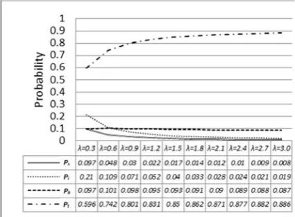
To evaluate the influences of data arrival rate, the arrival rate (

λ

) is changed from 0.3 to 3.0 with step 0.3 in corresponding to service rate (μ)=0.3, collision probability (Pc)＝0.1, threshold (N)=4 and queue size=7.

Figure 5 demonstrated that the system probability at sleep mode becomes small when the data arrival rate is increased. The USN has higher opportunity to receive data packet as well as to be woken up. The probability in idle state also becomes smaller because of receiving data quickly make the number of data in queue to be threshold N. The state is turned into busy mode. There are no close relation between arrival rate and busy state probability because of many other effects. The transmit probability is increased proportional to the data arrival rate (λ) since the service rate (μ) is less than arrival rate to result in staying at transmit state longer.

Figure 5: Data input rate(λ) and the variation of probability in different state

4.2 The Variation of System Service Rate

To evaluate the influence of changing service rate (μ) form 0.3 to 3, we assign the arrival rate (λ)=0.3,collision probability (P_c)=0.1, threshold (N)=4 and queue size(K)=7. The experimental result in Figure 6, it displays that the transmit probability is decreased if the service rate (μ) is increased. The probability toward the sleep state is increased as well as the idle state because of fixed arrival rate. The probability of busy state is decreased due to increasing service rate.

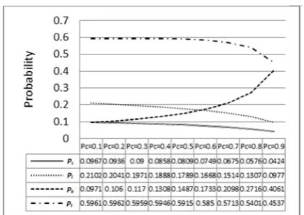
4.3 The Variation of Packet Collision

Probability

(7)

7 collision probability has big influence on the probability of busy state. The bigger busy state probability indicates that stay at the busy state longer. The probability for the rest state becomes small due to busy state probability increased.

Figure 6: System service rate (μ) and the variation of probability in different state

Figure 7: The probability of packet collision (P_c) and the variation of probability in different state

4.4 The Variation of Queue Threshold

In Figure 8, we change the value of threshold from 3 to k-2 when assuming service rate (μ)=0.3, arrival rate (λ)=0.3 and queue size (K)=12. The results show when the threshold is increased, the USN received more packets for turning its state from busy to idle. This increases the value of P_i. The higher value of the threshold is, the lower differences between N and K. This results in the probability of busy state reduced. Similarly, the probability of transmission state is also reduced because of more packets in queue for transmission.

Figure 8: Queue threshold (N) and the variation of probability in each state

4.5 The Threshold N of Lowest Power

Consumption

The threshold (N) of lowest power consumption is computed in this experiment,. The parameters for this experiment is: (N)=3~K-2, (μ)=0.3, (λ)=0.3, (P_c)=0.1 and (K)=12. Because the system power consumption should be calculated, the parameters are set as: Chold=5, Csetup=300, Cidle=50, Cbusy=500, Csleep=1 and Ctransmit=500.

Figure 9 shows that system power is in the lowest state when threshold is set to 6. This is useful for the parameter of setting threshold (N) for lowest power consumption to extend the life cycle of USN.

Figure 9: The threshold (N) of the lowest power consumption

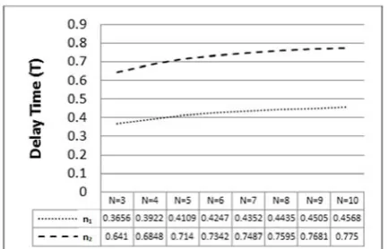
4.6 Packet Delay Time

In this experiment, the packet delay time is computed with the parameters: (N)=3~K-2, (μ)=0.3, (λ)=0.3, (P_c)=0.1, (K)=12. Figure 9 is the probability of two packets with different priorities stayed in sensor node. The packet delay time is calculated by multiplying T (working period). In Figure 10, n1 is the probability of packet with higher priority whose delay time is lower than n2.

N=3 N=4 N=5 N=6 N=7 N=8 N=9 N=10

Power 437.77 431.8 429.2 428.51 428.97 430.12 431.58 433

422 424 426 428 430 432 434 436 438 440

Po

w

er C

on

su

mp

tio

(8)

8 Figure 10: The packet delay time with a single sensor node

Figure 11 is the delay time when a packet transferred through three and ten sensor nodes. The higher value of N is, the longer time of packet is delayed. The delay time gap would be higher if the transfer frequency is increased.

5. Conclusions

In this research, we proposed a method for increasing the available time of system with lower cost by extending the usage of battery power. The sleep mode and limited queue of system is adopted in this research. By quantizing the variables of system power consumption, the best value of queue threshold can be obtained. This is useful for extending the power of USN. Besides, the priority is applied to the ubiquitous computing of packet. In this way, packet with higher priority can be transferred faster. This can be applied to the system with real time reaction.

Figure 11: The delay time with numerous sensor nodes

References

[1] O. Storz, A. Friday, N. Davies, J. Finney, C. Sas, and J. G.

Sheridan, “Public ubiquitous computing systems: lessons from the e-campus display deployments,” IEEE Pervasive Computing, vol. 5, no. 3, pp. 40–47, 2006.

[2] J. Hightower and G. Borriello, “Location systems for

ubiquitous computing,” IEEE Computer, vol. 34, pp. 57–66, Aug. 2001.

[3] I.F. Akyildiz, W. Su, Y. Sankarasubramaniam, and E. Cayirci.

“Wireless Sensor Networks: A Survey.” Computer Networks, vol.38, issue 4, pp.393-422, 15 March 2002.

[4] D. Culler and W. Hong, “Wireless Sensor Networks,”

Communications of the ACM, vol.47, issue 6, pp.30-33, June 2004.

[5] C. E. Jones, K. M. Sivalingam, P. Argawal and J. C. Chen, “A

Survey of Energy Efficient Network Protocols for Wireless Networks,” Wireless Networks, vol.7, pp.343-358, 2001.

[6] L. Wang and Y. Xiao, “A Survey of Energy-efficient

Scheduling Mechanisms in Sensor Networks,” Mobile Networks and Applications, vol.11, pp.723-740, 2006.

[7] Jian Li and Mohapatra, P., “An Analytical Model for the

Energy Hole Problem in Many-To-One Sensor Networks,” Vehicular Technology Conference, 2005. VTC-2005-Fall. 2005 IEEE 62nd, vol.4, pp.2721-2725, 25-28 Sept. 2005.

[8] J. Lian, K. Naik and G. Agnew, “Data Capacity Improvement

of Wireless Sensor Networks Using Non-uniform Sensor

Distribution,” International Journal of Distributed Sensor

Networks, vol.2, no. 2, pp.121-145, 2006.

[9] X. Wu, G. Chen and S. K. Das, “On the Energy Hole Problem

of Nonuniform Node Distribution in Wireless Sensor Networks,” in Proc. Third IEEE Int’1 Conf. Mobile Ad-hoc and Sensor Systems (MASS’06), pp.180-187, Oct. 2006.

[10]W. Zhang, H. Song and S. Zhu, “Least Privilege and Privilege

Deprivation: Towards Tolerating Mobile Sink Compromises in Wireless Sensor Networks,” in ACM MOBIHOC, May 2005.

[11]M. J. Miller and N. H. Vaidya, ”Minimizing Energy

Consumption in Sensor Networks Using a Wakeup Radio,” in IEEE WCNC 2004, March 2004.

[12]MICA2 Mote Datasheet,

http://www.xbow.com/Products/Product_pdf_files/Wireless_p df/6020-0042-02_A_MICA.pdf, 2004.

[13]X. Yang and N. H. Vaidya, “A Wakeup Scheme for Sensor

Networks: Achieving Balance between Energy Saving and End-to-end Delay,” in Proceedings of the 10th IEEE Real-time and Embedded Technology and Applications Symposium (RTAS’04), pp.19-26, 25-28 May 2004.

[14]Ye, W., Heidemann, J., and Estrin, D. “An Energy Efficient

MAC protocol for Wireless Sensor Networks,” in Proc. IEEE INFOCOM, pp.1567-1576, June 2002.

[15]W. Ye, J. Heidmann and D. Estrin, “Medium Access Control

with Coordinated Adaptive Sleeping for Wireless Sensor Networks,” IEEE Transactions on Networking, vol.12, no. 3, pp.493-506, June 2004.

[16]Fuu-Cheng Jiang, Der-Chen Huang, Chao-Tung Yang and

Fang-Yi Leu, “Lifetime Elongation for Wireless Sensor

Network Using Queue-based Approaches,” Journal of

Supercomputing. (Springer link)

Kuo-Hsiung Wang, “Mitigation Techniques for the Energy Hole Problem in Sensor Networks using N-policy M/G/1

Queuing Models,” The IET International Conference on

Frontier Computing-Theory, Technologies, and Applications (IET FC 2010), pp.281-286, August 4-6, 2010, Taichung, Taiwan.

Kuo-Hsiung Wang, “Design Framework to Optimize Power Consumption and Latency Delay for Sensor Nodes using

Min(N, T) Policy M/G/1 Queuing Models,” 5th_{International}

Conference on Future Information Technology (FutureTech 2010), pp.1-8, 20-24 May 2010, Busan, Korea.

[19]Fuu-Cheng Jiang, Der-Chen Huang and Kuo-Hsiung Wang,

“Design Approaches for Optimizing Power Consumption of

Sensor Node with N-Policy M/G/1 Queuing Model,” 4th

International Conference on Queuing Theory and Network Applications (QTNA 2009), July 29-31, 2009, Fusionopolis, Singapore.

[20]J. Polastre, J. Hill and D. Culler, “Versatile Low Power Media

for Wireless Sensor Networks,” in Proc. ACM SenSys, pp.3-5, Nov. 2004.

[21]C. Schurgers, V. Tsiatsis and M. Srivastava, “STEM:

Topology Management for Energy Efficient Sensor Networks,” Aerospace Conference Proceedings, 2002, IEEE, vol.3, pp.3-1099~3-1108, 2002.

[22]R. Davis and A. Wellings, “Dual priority scheduling,” in

Proceedings of the 16th IEEE Real-Time Systems Symposium, pp.100–109, 1995.

[23]http://www.cs.cmu.edu/~osogami/thesis/html/node86.html

[24]http://www.cs.cmu.edu/~osogami/thesis/html/node91.html