COMPARATIVE ASSESSMENT OF RADIAL BASIS FUNCTION NEURAL
NETWORK AND MULTIPLE LINEAR REGRESSION APPLICATION
TO TRIP GENERATION MODELLING IN AKURE, NIGERIA
ETU Japheth Eromietse1, Oyedepo Olugbenga Joseph2
1,2 Department of Civil Engineering, Federal University of Technology, Akure, Ondo State, Nigeria
Received 24 January 2019; accepted 20 March 2019
Abstract: Efficacy of using Radial Basis Function Neural Network (RBFNN) and Regression Models (MLR) to estimate trip generation rates in Akure, Nigeria was compared. This sterns from a desire to test more novel modelling techniques besides regression which has hitherto been used in the study area. Data for the study were collected through household questionnaire interview survey in the study area between October 2017 and January 2018. SPSS 22 was used in carrying out data analysis. Correlation analysis showed that Number of household
members, (NHM), Number of employed household members, (NEHM), Number of students in
household (NSH), Number of Household members with age greater than 12years, (NHM12) and
Number of Driver’s license holders in the household, (NDLH) were the household variables
having significant influence on home based trips generation rates. The models were compared
and validated using their R2 values and Relative Error (RE). Modelling results showed that
RBFNN displayed higher accuracy with R2 value of 0.947 and RE of 0.391 as compared to
MLR with R2 value of 0.589 and RE of 0.875. The study was able to uphold the capability of
artificial neural networks to produce better results in travel demand forecasting areas than regression techniques.
Keywords: artificial neural network, radial basis function, regression, model, trip generation, travel demand.
1 Corresponding author: [email protected]
1. Introduction
It is estimated by the Global Traffic Volume forecast that traffic congestion in cities would double between 1990 and year 2020 and also double by 2050 (Engwitch,1992). This is an indication of what the future congestions would cause for people living in urban environment if not properly managed. Akure, a city in Nigeria which is a developing African country is plagued with its own share of the transportation problems arising from
carried out a study highlighting the indices of traffic congestion in Akure metropolis and made a ten-year projection to 2025 which indicated unfavourable level of service with severe congestion on these major arterials by 2025. With the high levels of congestions and unfavourable level of service (LOS) exhibited by major road networks in Akure, it is imperative to characterise the factors affecting travel patterns within the city.
An estimation of travel demand is a necessary precursor to provision of facilities to tackle anticipated transportation problems in an urban area. The traditional travel demand analysis procedure consists of trip generation, trip distribution, modal split and traffic assignment. According to Sarkar et al., (2015) multiple linear regression analysis is the statistical technique most often used to derive the estimates of trip generation, where two or more independent factors are assumed to be simultaneously affecting the amount of travel. They stated that this technique measures separate influence of each factor acting in association with the other factors. The aim of such technique is to estimate future trips from any zone, given the values of a set of land use and socio-economic parameters. This regression analysis has been used over time to estimate trip generation rates in the study area by authors such as Busari et al., (2015a), Busari et al., (2015b), Ogunbodede and Ale (2015), Okoko and Fasakin (2007) etc. However, with advances in the field of Artificial
Intelligence (AI), an alternative approach for addressing this problem is by using Artificial Neural Networks. Applications of Artificial Neural Networks have produced excellent results in many areas of research. Neural Networks have become well known as ‘universal approximators’. Therefore, this research explored the suitability of the Radial Basis Function Neural Network (RBFNN) and Multiple Linear Regression Models (MLR) in predicting number of home-based trips generated in the study area. Assessment of their suitability will be carried out using certain parameters to measure the accuracy of their estimates.
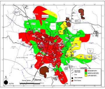
1.1. The Study Area
Fig. 1.
Map of Akure Showing the Study Locations Source: Fasakin et al., (2018)
2. Literature Review
2.1. Existing Trip Models in the Study
Area
Busari et al., (2015) investigated the influence income and car ownership on recreational trip pattern in Akure metropolis, focusing on the frequency of trips, modal choice and the landuse pattern. The study established the fact that modal choice may not necessarily be a function of household income. Ogunbodede
concluded that in-vehicle travel time is germane to modal choice in the study area. Okoko and Fasakin (2007), developed trip generation models for low, medium and high-density areas in Akure Metropolis. They developed trip rate predictive models using the multi-variable regression model. They concluded that differential in trip rates in the various residential density zones in Akure is not significant and it could therefore be concluded that residential density types in Akure do not significantly influence trip generation rates in the town.
These studies have been able to use regression models to show the influence of some socio-economic characteristics and commuter characteristics on trip rates and modal choices in the study area. This current study is an attempt to deviate from the use of regression models in analysing travel demand by engaging Radial Basis Function Neural Network (RBFNN) and hence establish a basis for comparing the suitability of the duo.
2.2. Artificial Neural Networks in Travel
Demand Modelling
Artificial neural networks (ANN) are inspired by the biology of a brain’s neuron. Its application is driven by the motivation of various researchers to incorporate human intelligence into machines so that they can also perform certain complex tasks easily. The network is configured to make use of artificial neurons which are characterised and organised in a way that is evocative of the human brain. The ANN thereby possesses an impressive number of the brain’s properties such as learning from experience, generalization from previous instances and apply to new data, etc. (Edara, 2003). ANNs are one of the most realistic models of the biological brain functions (Ferentinou and
Sakellariou 2007), and can be considered. as an efficient way for solving the complex problems. The ability of the ANN to classify, examine, simulate and make decisions from varying data inputs has given them a wide application in the engineering field, and even in other fields.
not always perform better than logit model stating that ANN models are sometimes performing equally well or even worse than logit model. They stated that performance of the model depended on the configuration of the network and the background knowledge of the researchers. Review of previous studies have shown diverse areas wherein ANN have been used to develop transport models. The studies have also given divergent views on the superiority of the ANN models to traditional regression models in travel demand modelling. This paper compares the suitability of trip generation models developed with both ANN and Multiple regression thereby providing a basis for measuring their accuracy, efficiency and superiority in predicting trip rates in the study area.
3. Methodology
3.1. Data Collection
Data for the study were sourced through a household questionnaire interview survey carried out in the study area between October 2017 and January 2018. The study area was divided into three residential density zones namely Low density zone, Medium density zone and High density zone. Different locations were selected from the residential density zones. The residential density zones division were contiguous to that of Okoko and Fasakin (2007) and Fasakin et al., (2018) as shown in Figure 1.
T he Sy stemat ic R a ndom Sa mpl i ng Technique was used in carrying out the travel survey. In using this method, every
3rd household along a street of a study
location was selected for the survey. The questionnaire used for the survey contained questions on household characteristics such
as Gender, age, economic status, number of household members, Number of cars available for use by household members, the number and type of driving licences owned by household members and other household attributes. Household members of 12 years and above were also required to fill a travel diary of trips they embarked on the previous day. The survey had retrospective character and the respondents were asked about all their trips from the previous day. The travel diary section of the questionnaire included questions concerning travelling (e.g. origin and destination address, mode of transport, trip purpose etc.). A full interview with a household lasted approximately 30 minutes.
Data obtained from the household survey were subsequently analysed using Statistical Package for Social Sciences Version 22 (SPSS 22). SPSS 22 was used in carrying out descriptive statistical analysis, bivariate analysis as well as predictive model formulation.
3.2. Variable Selection
3.3. RBFNN Topology and Development
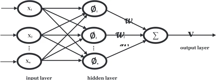
The Radial Basis Function Neural Network (RBFNN) which is a feedforward neural network that consists of three layers: input layer, hidden layer and output layer was used in developing a trip generation model to determine the daily home-based trip rates from the study area. Figure 2 shows the typical architecture of a RBFNN used in this study. In using the RBFNN, there is no calculation in input layer nodes. The input layer nodes only pass the input data to the
hidden layer. The input layer consist of ns
nodes where input vector x = (x1, x2,…, xns).
The hidden layer consists of n nodes and each hidden node j = 1, 2,, n has a centre
value cj. Each hidden layer node performs a
nonlinear transformation of the input data onto new space through the radial basis function. The number of hidden units is determined by the testing data criterion:
The best number of hidden units is the one that yields the smallest error in the testing data. The radial basis function used in this study was the Gaussian function given by Eq. (1):
(1)
where x - cj represents the Euclidean distance
between input vector (x) and the radial basis function centre (cj) while rj is the width of
radial basis function.
The resulting output layer from the transformation is linear, and of the form in Eq. (2):
(2)
where wj is the connection weight of hidden
layer to output layer and n is number of hidden node.
Fig. 2.
Typical Architecture of RBFNN Used in the Study Source: Drawn by Authors (2018)
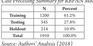
In developing the network for this study, the data set was divided into three parts namely: Training (61.2%), Testing (27.8%) and validation (10.9%). The training process involves making the network adapt
optimum number of hidden nodes. The OLS procedure, chooses the radial basis function centre one by one in a rational way until an adequate network with optimum numbers of hidden nodes and their centres have been constructed. Once the centre and optimum number of hidden nodes have been determined, the connection weights of the hidden layer to output
layer were automatically activated. The validation data-set was used to stop the learning process (assess the learning of the network during training) and all testing data-set was used to assess the RBFNN model’s performance after completion of the training process. Table 1 shows number of data used at the different stages of the RBFNN.
Table 1
Case Processing Summary for RBFNN Model
N Percent
Training 1200 61.2%
Testing 545 27.8%
Holdout 214 10.9%
Total 1959 100.0%
Source: Authors’ Analysis (2018)
3.4. Validation of RBFNN Model
Three measures were used to assess the performance and hence the validity of the model. This first validation test involved testing the ability of the model to generalise their forecasting beyond the training data and to perform well when stranger data sets are inputted. If the network can generalize rather precisely the output for this testing data in same way as the training data then it means that the neural network is able to predict the output correctly for new data and hence the network is validated.
Second measure of validation was the Coefficient of determination (R2). The R2 is a measure of the strength of the relationship between variables. It ranges between 0 and unity. A value of unity indicates that the model explains all the variability of the response data around its mean. The weakest linear relationship is indicated by a value equal to 0. However, values of 0.5 are
acceptable to establish relationships between variables and this was the standard adopted in this research.
Thirdly the magnitude of Relative Error between the predicted and observed values was also used in testing the validity of the model. The error values between the observed survey results and the predicted results with the RBFNN model are expressed by Eq. (3).
(3)
Where MO is the observed mean value
of home-based person trips and MP is
the predicted mean value of home-based person trips. A 5% threshold was set as the acceptable level of error values for the study. This standard was used to check the validity of the models.
3.5. Multiple Linear Regression Model
(MLR)
The Multiple Linear Regression Model (MLR) was also used in developing trip generation models to determine the daily home-based trips rates from the study area. The MLR takes the form in Eq. (4):
(4)
Where Tij is number of home-based trips
generated by households daily, ß0 is the
model constant while ß1 - ßn are regression coefficients associated with the household characteristics X1 – Xn.
The technique measures the influence of each factor acting in association with the other factors on the number of trips. The aim of such equation is to estimate future trips from any zone, given the values of a set of land use and socio-economic parameters. This study employed the stepwise regression procedure of regression analysis in developing the MLR model. The MLR model was validated using the R2 and Relative Error already described above.
3.6. Model Comparisons
To assess the suitability, quality and efficacy of the two models in predicting the number of
home-based trips generated from households in the study area, comparisons were drawn between their results. These comparisons were carried out based on the values of their respective R2 and Relative Error.
4. Results and Discussion
4.1. Descriptive Statistics of Household
Travel Characteristics
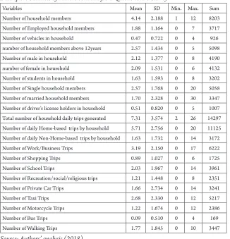
From the survey carried out about 187 (10%) questionnaires were returned from the low density zone while 788 (40%) and 1005 (50%) were returned from the medium and high density zones respectively. This makes a total of 1980 interviewed households. Also about 5098 household members of age 12 and above filled the travel diary. The travel diary yielded a total of 14297 trips from the households daily. Table 2 shows the data obtained from the household interview survey. The mean and standard deviation of these data are as shown.
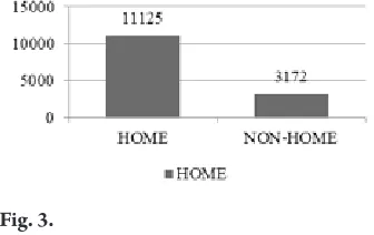
Results from Figure 3 showed that of the 14297 trips generated from the questionnaire survey, 11125 where home-based trips while 3172 were non-home-based trips. This revealed that most of the trips generated within the study area are home-based trips.
Fig. 3.
Trip Categories
Table 2
Descriptive Statistics of Factors obtained from Questionnaire Survey
Variables Mean SD Min. Max. Sum
Number of household members 4.14 2.188 1 12 8203
Number of Employed household members 1.88 1.164 0 7 3717
Number of vehicles in household 0.47 0.722 0 4 926
number of household members above 12years 2.57 1.434 0 5 5098
Number of male in household 2.12 1.377 0 8 4190
number of female in household 2.09 1.531 0 6 4132
Number of students in household 1.63 1.593 0 8 3202
Number of Single household members 2.57 1.768 0 20 5058
Number of married household members 1.70 2.328 0 30 3347
Number of driver’s license holders in household 0.51 0.820 0 5 1007 Total number of household daily trips generated 7.31 3.574 2 26 14297 Number of daily Home-based trips by household 5.71 2.756 0 20 11125 Number of daily Non-Home-based trips by household 1.63 1.732 0 14 3172
Number of Work/Business Trips 3.19 2.150 0 17 6222
Number of Shopping Trips 0.89 1.027 0 6 1725
Number of School Trips 2.03 1.967 0 14 3961
Number of Recreation/social/religious trips 1.21 1.448 0 8 2351
Number of Private Car Trips 1.66 2.734 0 14 3241
Number of Taxi Trips 2.68 2.330 0 12 5217
Number of Motorcycle Trips 1.22 1.674 0 12 2386
Number of Bus Trips 0.09 0.510 0 4 169
Number of Walking Trips 1.77 1.845 0 10 3447
Source: Authors’ analysis (2018)
4.2. Number of Trips per Household
The number of trips per household surveyed in the study area are shown in Figure 4. It reveals that the highest trip per household was from the low density zone with 8.53 person trips per household. The high
Fig. 4.
Number of Trips per Household Source: Authors’ analysis (2018)
4.3. Pearson Correlation Analysis
Results of the Pearson correlation analysis are as shown in Table 3. The coefficients showed that Number of household members,
(NHM), Number of employed household
members, (NEHM), Number of students in
household (NSH), Number of Household
members greater than age 12 (NHM12)
and Number of Driver’s license holders
in the household (NDLH) had coefficients
greater than 0.50 thereby indicating strong correlation with the number of home-based trips generated. Therefore, the variables were selected as the independent variables to be used in this study and their effect on Number of home-based trips will be assessed.
Table 3
Pearson Correlation Coefficients of Variables Used in the Models
NHB NHM NEHM NSH NHM12 NDLH
Number of Home-based trips, NHB 1.000 0.703 0.535 0.541 0.598 0.504
Number of household members, NHM 0.703 1.000 0.319 0.466 0.465 0.277
Number of employed Household Members, NEHM 0.535 0.319 1.000 0.109 0.426 0.275
Number of Students in Household, NSH 0.541 0.466 0.109 1.000 0.400 0.220
Number of Household Members above age 12, NHM12 0.598 0.465 0.426 0.400 1.000 0.361
Number of Driver’s License Holders in Household, NDLH 0.504 0.277 0.275 0.220 0.361 1.000
Source: Authors’ analysis (2018)
4.4. MLR Model Results
The MLR model developed with combined data from the three zones showed from Table 4 that all the independent variables
a positive relationship with the number of home-based trips generated across the three zones.
(5)
The MLR model shows that all variables considered have positive coefficients. This implies that there will be a corresponding rise in the number of home-based trips generated in Akure with a unit increase in any of the variables.
Table 4
Coefficients of MLR Model
Variables B Standard Error t Sig.
(Constant) 1.692 0.095 17.743 0.000
NHM 0.465 0.033 13.979 0.000
NHM12 0.275 0.044 6.238 0.000
NDLH 0.354 0.054 6.506 0.000
NSH 0.332 0.038 8.781 0.000
NEHM 0.329 0.051 6.491 0.000
Source: Authors’ analysis (2018)
With the coefficients from Table 4 the mean number of predicted home-based trips across the zones using MLR was computed to be 5.66, which translates to a total of about 11088 home-based trips.
4.5. MLR Model Validation
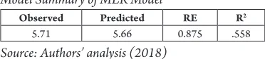
The MLR model yielded an R2 value of 0.558.
This is higher than the value of 0.5 adopted
as the standard R2 value in this study. The
value implies that the model was able to
explain 55.8% of the relationship between the dependent and independent variables. This served to validate the MLR model. Also, the Relative Error between the observed number of home-based trips and that predicted by the MLR model was 0.875%. This shows a relative closeness between the predicted and observed values thereby depicting a high level of accuracy in the prediction of the MLR model. This also served to validate the MLR
model. The R2 and RE values of the MLR
model are shown in Table 5.
Table 5
Model Summary of MLR Model
Observed Predicted RE R2
5.71 5.66 0.875 .558
Source: Authors’ analysis (2018)
4.6. RBFNN Model Results
About 61.2%, 27.8% and 10.9% respectively of the data were used for the training, testing and validation analysis. The network used
in developing the RBFNNmodel comprised
of 1 hidden layer with 9 neurons. The architecture for the network is shown in Figure 5.
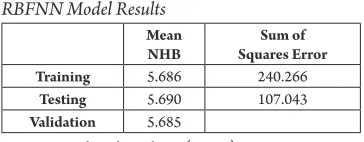
number of home-based trips as 5.686, 5.690 and 5.685 respectively for the training, testing and validation stages respectively. Considering the testing stage results, a total of 11147 trips were
predicted for the study area using the RBFNN for a mean number of 5.69 home-based trips. The model also displayed favourable sum of square values as seen in Table 6.
Fig. 5.
RBFNN Model Architecture Source: Authors’ analysis (2018)
Table 6
RBFNN Model Results
Mean
NHB Squares ErrorSum of
Training 5.686 240.266
Testing 5.690 107.043
Validation 5.685
Source: Authors’ analysis (2018)
4.7. RBFNN Model Validation
It is also worthy to note the consistency observed in the predicted results of the training testing and validation samples. This implies that the RBFNN could predict the number of home-based trips generated in the study with high consistency. This consistency in results goes to validate and uphold the accuracy of the RBFNN.
The RBFNN model gave an R2 value of
Table 7
RBFNN Model Summary
Observed Predicted RE R2
Training
5.71
5.686 0.407
0.947
Testing 5.690 0.391
Holdout 5.685 0.422
Source: Authors’ analysis (2018)
4.8. Comparing the RBFNN and MLR
A comparative assessment of the results of MLR and RBFNN models showed that the RBFNN performs better for predicting
home-based trips in the study area. This can be seen from Table 8. The RBFNN performed better
with R2 value of 0.947 as compared to 0.558
of the MLR while also displaying a lower RE of 0.391% compared to 0875% of the MLR.
Table 8
Performance Measure of the MLR and RBFNN
Model R2 RE
MLR 0.558 0.875
RBFNN 0.947 0.391
Source: Authors’ analysis (2018)
5. Conclusion
This research explored the suitability of the Radial Basis Function Neural Network (RBFNN) and Multiple Linear Regression Models (MLR) in predicting number of home-based trips generated in Akure, Nigeria. Data were obtained from households in the study area through a household questionnaire interview survey.
Correlation analysis helped in identifying factors/variables which mainly influence home-based trips generation rates in the study area. The correlation analysis showed
that number of household members, (NHM),
number of employed household members,
(NEHM), number of students in household
(NSH), number of Household members with
age greater than 12years (NHM12) and number of Driver’s license holders in the household,
(NDLH) were highly correlated with the
number of daily home-based trips and as such were selected as the independent variables for the various trip generation models. In the aggregate model of trip generation developed with aggregate data from the three zones, the
RBFNN with R2 value of 0.947 was found
to be more accurate than the MLR with R2
value of 0.589. The RBFNN also showed better performance in terms of the Relative Error between the observed and predicted values. Whereas the RBFNN had a RE of 0.391, that of the MLR was 0.875.
modelling and serve as improvement on the traditional travel demand modelling methods using regression analysis. This study recommends that transport researchers make use of the RBFNN in modelling home based trip generation rates in the study area as it has proved more accurate in this study than the MLR which has been used previously.
References
Ajayi S. A.; Owolabi A. O.; Busari A. A. 2016. Measures that Enhance Favourable Levels of Service and their Modes of Sustainability on Major Roads in Akure, South-Western Nigeria. In Proceedings of 3rd International Conference on African Development Issues (CU-ICADI 2016),
329-336.
Arliansyah, J.; Hartono, Y. 2015. Trip attraction model using radial basis function neural networks, Procedia Engineering 125: 445-451.
Busari, A. A.; Owolabi, A. O.; Modupe, A. E. 2015a. Modelling the Effect of Income and Car Ownership on Recreational Trip in Akure, Nigeria, International Journal of Scientific Engineering and Technology 4(3): 228-230.
Busari, A. A.; Owolabi, A. O.; Fadugba, O. G.; Olawuyi, O. A. 2015b. Mobility of the Poor in Akure Metropolis: Income and Land Use Approach, Journal of Poverty, Investment and Development15: 28-33.
Celikoglu, H. B.; Cigizoglu, H. K. 2007. Modelling public transport trips by radial basis function neural networks,
Mathematical and computer modelling 45(3-4): 480-489.
Edara, P. K. 2003. Mode choice modelling using artificial neural
networks [PhD Thesis]. Virginia Tech, USA.
Engwitch, D. 1992. Towards an Eco-City; Calming the Traffic. Envirobook Publishers, Australia.
Fasakin, J. O.; Basorun, J. O.; Bello, M. O.; Enisan, O. F.; Ojo, B.; Popoola, O. O. 2018. Effect of Land Pricing on
Residential Density Pattern in Akure, Nigeria, Advances in Social Sciences Research Journal 5(1):31-43.
Ferentinou, M. D.; Sakellariou, M. G. 2007. Computational intelligence tools for the prediction of slope performance, Computers and Geotechnics34(5): 362-384.
Laoye A. A.; Owolabi A. O.; Ajayi S. A. 2016. Indices of Traffic Congestion on Major Roads in Akure, a Developing City in Nigeria, International Journal of Scientific & Engineering Research 7(6): 434-443.
Millennium Cities Initiatives. 2017. Akure, Nigeria. Available from internet: <http://mci.ei.columbia.edu/ millenium-cities/akure-nigeria/>. Accessed November 20, 2017.
Mozolin, M.; Thill, J. C.; Usery, E. L. 2000. Trip distribution forecasting with multilayer perceptron neural networks: A critical evaluation, Transportation Research Part B: Methodological34(1): 53-73.
Ogunbodede, E. F.; Ale, A. S. 2015. The Use Regression Model in the Forecast of Travel Demand in Akure, Nigeria, Annals of the University of Oradea, Geography Series/ Analele Universitatii din Oradea, Seria Geografie 2: 186-194.
Okoko, E.; Fasakin, J. O. 2007. Trip Generation Modelling in Varying Residential Density Zones: An Empirical Analysis for Akure, Nigeria, The Social Sciences2(1): 13-19.
Owolabi, A.O. 2009. Paratransit Modal Choice in Akure, Nigeria - Applications of Behavioural Models, ITE Journal
79(1): 54-58.
Sarkar, P. K.; Maitri, V.; Joshi, G. J. 2015. Transportation planning: principles practices and policies. First edition.PHI Learning Pvt. Ltd. Delhi.