OPTIMIZE THE POWER CONTROL AND NETWORK LIFETIME USING ZERO - SUM GAME THEORY FOR WIRELESS SENSOR NETWORKS

(1)

577 |

P a g e

OPTIMIZE THE POWER CONTROL AND NETWORK

LIFETIME USING ZERO - SUM GAME THEORY FOR

WIRELESS SENSOR NETWORKS

Vinoba.V

1

, Chithra.S.M

2

1

Department of Mathematics, K.N. Government Arts college, Tamil Nadu,( India.

)

2

Department of Mathematics, R.M.K College of Engineering and Technology, Research

Scholar, Bharathidasan University, Tamil Nadu, (India.)

ABSTRACT

A wireless sensor network is one of the most attractive research fields in the communication networks. This will

creates a great popularity regarding their potential use in a wide variety of applications like monitoring

environmental attributes, intrusion detection, and various military and civilian applications. The main

performance of these sensor networks is maintaining network life time while satisfying coverage and

connectivity in the deployment region. In this paper, we look at the problem of maintaining energy level of the

sensor node , reliable routing and multi-hop in WSN within a finite two-person zero-sum game theoretic

approach. The game theoretic scheme is based on models that express the interaction among players, in this

case, nodes, by modeling them as elements of a social networks in such a way that they act as to maintaining the

maximum utility. Simulation results are shows the effectiveness of the proposed game with various path loss

exponents and also the proposed games is able to maintain the energy level of the network life time.

Keywords:

Wireless Sensor Networks, Two-person zero-sum Game Theory, Routing, Life time

.

I. INTRODUCTION

Wireless Sensor networks is one of the most promising and interesting areas in the past years. This network

consists of a large number of sense nodes. These nodes are able to gather the information and process it and

send it to the relevant destinations. Also, these nodes form a network by communicating with each other either

directly or through other nodes. One or more nodes among them will serve as sink(s) that are capable of

communicating with the user either directly or through the existing wired networks. The primary component of

the network is the sensor, essential for monitoring real world physical conditions such as sound, temperature,

humidity, intensity, vibration, pressure, motion, pollutants etc. at different locations. The nodes are deployed in

hostile environment it is not feasible to replace the batteries. Therefore energy conservation is very crucial for

WSN’s both for each sensor node and the entire network level operations to prolong the network lifetime.

Energy –constrained networks, such as Wireless sensor networks are composed of nodes typically powered by

batteries, for which replacement or recharging is very difficult, if not impossible. With finite energy, we can

only transmit a finite amount of information. Therefore, minimizing the energy consumption for data

transmission becomes one of the most important design considerations for such networks [1]. One of the desired

(2)

578 |

P a g e

inaccessible terrains in which up to data monitoring schemes are unsafe, heavy-handed, and sometimes

infeasible.

Now days, some research efforts have focused on establishing efficient routing paths for transmitting packets

from a sensor node to a sink in WSN’s. Routing means finding the best possible way for data transmission from

source node to the destination node in the network by considering networks parameters. The other important

factor that must be considered in the network is Load Traffic Distribution. Usually the traffic load in wireless

sensor networks is unbalance. For example, sensors which are nearer to the source have more data load.

Therefore, optimization of load distribution, called Load Balancing, is one of the important factors for

improving the efficiency of the networks. Optimization of load traffic distribution in WSN could increase the

lifetime of the network. Since, there is more power consumption in nodes with more traffic load then the data

transaction in the network could be optimized.

Game Theory is based on models that express the interaction among players, in this case nodes, by modeling

them as an element of a social networks in such a way that they act to maximize their own utility. This allows

the analysis of existing algorithms and protocols for WSN’s as well as the design of equilibrium-inducing

mechanisms that provide incentives for individual nodes to behave in socially constructive ways. In this paper,

by using Zero-Sum Game Theory approach for WSN, optimal route in WSN is found. In this approach, routing

and sensor nodes are assumed to be the game and players respectively. All players want to increase their benefit.

So we use a mixed strategy model as well as profit and loss calculation for each player.

II. RELATED WORKS

The main goal of routing in WSNs is to guarantee successful packet delivery from source to sink node under

constraint requirements like energy consumption, end to end delay, packet delivery ratio and QoS etc. In

addition to energy consumption, more challenges and design issues are pointed out [1].

Lifetime is the one of main design issue in WSN and the lifetime of the sensor node is mainly depends on the

battery energy level. Since WSN is composed of very small nodes, their energy resources are very limited this

imposes tight constraints on the operation of sensor nodes. The transceiver is the element which drains most

power from the node (Fedora and Collier 2007), thus the routing protocols will significantly influence the

lifetime of the overall network.

Energy-aware Routing protocol (Shah and Rabaey 2002) is similar to directed diffusion with the difference is,

it maintains a set of paths instead of or enforcing one optimal path. These paths are maintained and chosen by

means of a certain probability, which will depend the energy consumption of each path. By selecting different

routes at different times, the energy of any single route will not deplete so quickly, the network lifetime

increases.

Data centric, hierarchical and location based routing protocols gives the importance on energy efficiency and

increased network lifetime, with little concern on quality measures. This group of routing protocols in addition

to the energy efficiency focuses on QoS metrics such as latency, bandwidth and efficiency. QoS based protocols

(3)

579 |

P a g e

reliable routing algorithms. These protocols are concerned on the network fault tolerance and resilience of the

network on node failures or node malfunctioning.

III. MATHEMATICAL MODEL

Game Theory is a theory of decision making under conditions of uncertainly and interdependence. In the

distributed sensor network the game equation has to be found, with application of a game strategy. It is assumed

that all the nodes in the sensor networks are the same and that all nodes are in the interference range. The

activity of all the nodes is at the same level and it increases with the increase of power level transmission.

A game has three components:

(i) a set of players (ii) a set of possible of actions for each player and (iii) a set ofstrategies.

A player’s strategy is a complete plan of actions to be taken when the game is actually played. Players can act

selfishly to maximize their gains and hence a distributed strategy for players can provide an optimized solution

to the game. In any game, utility represents the motivation of players. A utility function, describing player’s

preferences for a given player assigns a number for every possible outcome of the game with the property that a

higher number implies that the outcome is more preferred.

A Zero-sum game is a mathematical representation of situation in which a participant’s gain or loss of utility is

exactly balanced by the losses or gain of the utility of the other participants. The present survey covers research

on infinite zero-sum two-person games in normal form [3] .( i.e., zero-sum two-person games with infinite sets

of player strategies in which the player strategies are elements of certain abstract sets. In this article we do not

consider dynamic and differential games.

Definition: 3.1. The zero-sum two-person game in normal form is formally defined as a triple   X,Y,P

in which X and Y are arbitrary infinite sets representing the sets of strategies of Players I and II

respectively and P is a real function defined on the set X Y of all situations and is called the payoff

function or kernel of the game. (If P : X Y  R is the payoff function of Player I. Player II’s payoff in the

situation



x,y



is



 P



x,y





, where x X , yY the game being zero-sum)

Definition: 3.2 The existence of optimal (  optimal) strategies for the opponents in a zero-sum two-person

game is equivalent to satisfaction of the following equations:

X x

max

Y y

inf P



x,y

= υ --- (3.2)

The quantity υ is called the value of the game. Even in the simplest cases, however, equations (1) and (2) fall

short of being satisfied. Their proof requires the imposition of rather stringent algebraic constraints on the

strategy sets X , Y and the function P (such as concavity in xand convexity in y ) as well as topological

constraints ( the sets X and Y are topological spaces, and the function P has properties of the continuity

(4)

580 |

P a g e

It is reasonable, therefore, to extend the strategy sets of the players in such a way that the payoff function,

now defined on a new extended set of situations, will satisfy the required constraints .The extended strategy sets

must be convex and include the usual strategies.

Let  algebra of subsets of X _{containing all one-element subsets, let} _{be a}

algebra of subsets of Y _{, and let the function}P _{be bounded and measurable under the} algebra  x

 . A probabilistic measure defined on 

 

 is called a mixed strategy of Player I (II). If  is a mixed

strategy of Player I and  is a mixed strategy of Player II, then the payoff function P



,



under the

conditions of the mixed situation



,



is defined by the integral



,



P = P



x y

    

d x d y

X Y

 

 

, .

If the set of pure strategies of a player is infinite (and especially if it is denumerable ), then in the choice of

his set of mixed strategies there is a certain arbitrariness, which rests on the particular choice of algebra of

subsets of the pure strategy set on which the probabilistic measure is defined[2] .Various randomizations of pure

strategy sets have been investigated by Wald and Bieriein .Clearly, the sets of mixed strategies are convex and,

if the ordinary, or so-called pure, strategies are regarded as corresponding degenerate measures, include all the

pure strategies of the players. Under the conditions of mixed strategies the payoff function turns out be linear in

each of the variables.

Theorems establishing the validity of equations (1) and (2) for an infinite game or its mixed extension are

called existence theorems (or minimax theorems). The proof of existence theorem, (i.e.) the identification of

classes of games for which a value of the game exists (or does not exist), is one the fundamental problems of the

theory of infinite zero-sum two-person games [4].

A pair of optimal strategies of each player in a zero-sum two-person game ( or the set of  optimal

strategies for each player) in conjunction with the process of finding those strategies is known as a solution of

the game.

In the infinite game, as in any zero-sum two-person game  X,Y,P the principle of player’s optimal

behavior is the saddle point (equilibrium) principle.

Definition: 3.3. Saddle point

P ,   ,   , --- (3.3)

holds for allx X , yY is called saddle point.

This principle may be realized in the game if and only if  = 

 = 

 = P



x, y



where



 =

X x

max

Y y

inf P



x, y



_---_(3.4)



 = Y y min

X x

(5)

581 |

P a g e

(i.e) the external extreme of maximin and minimax are achieved and the lower value of the game _ is equal to

upper value of the game 

 . The game _{for which the (4) holds is called}_{strictly determined}_{and the number}

x, y



 --- (3.5).

The point



x,y



for which equation (5) holds, is called the  Saddle point and the strategies x & y

are called  optimal strategies for the players I and II, respectively.

NOTE:

Compare the definitions of the saddle point equation (3) and the   Saddle point equation (5), A deviation

from the optimal strategy reduce the player’s payoff where as a deviation from the   optimal strategies may

increase the payoff by no more than_.

In conclusion we will point out a special class of zero-sum two-person game in which

X ₌Y _{= [0, 1]. In these games, situations are the pairs of numbers}



x, y



_{, where}x, y

 

0,1 _{such games are}

called the games on the unit square. The class of the games on the unit square is basic in examination of

infinite games.

Example 1:

Suppose each of the players I and II chooses a number from the open interval (0,1). Then Player I receives a

payoff equal to the sum of the chosen numbers. In the manner we obtain the game on the open unit square with

the payoff function P



x, y



for Player I.



x y



P ,

=x  y, x

 

0,1 , y 

 

0,1 ---(3.6).

Here the situation (1,0) would be equilibrium if 1 and 0 were among the players’ strategies, with the game

value  being  1Actually the external extreme in (4) are not achieved but in the same time the upper value

is equal to the lower value of the game. Therefore  =1 and Player I can always receive the payoff sufficiently

close to the game value by choosing a number 1-_,

_{>0 as a sufficiently small number (close to 0), Player II can guarantee that his loss will be arbitrarily close to}

the value of the game.

The following theorem yields the main property of  optimal strategies.

Theorem1: For the finite value  _{of the zero-sum two-person game}  X,Y,P _{to exist, it is necessary}

and sufficient that, for any >0, there be  optimal strategies x,yfor the players I and II, respectively,

in which case



_ _



 P x , y

lim

0

(6)

582 |

P a g e

Proof

Case (i) first to prove the Necessary condition:

Suppose the game has the finite value . For any >0 we choose strategy xfrom the condition



_



   2 ,y x P Sup X x --- (3.8)

And strategy x from the condition



_



     2 , y x P Inf Y

y --- (3.9)

We know that 

 = X x max Y y

inf P

P  _{--- (3.10) for all strategies}x,y_.

Consequently,



,



₂

  



 y 

x P

--- (3.11)

 P x ,y

lim

0

=  follows from



_



   2 ,y x P Sup X x

and





 

    2 , y x P Inf Y

y .



_



   2 ,y x P Sup X x 





2 ,     y x P Inf Y y

Case (ii) Next to prove the sufficient condition:

_{hold for any number} 0_{, then}























 





              2 2 , 2 , , , , _ _ 

 Inf Sup P x y Sup P x y P x y Inf P x y Sup Inf P x y

y y X x Y y X x X x Y y --- (3.12)

Hence it follows that _ _



  _{, the inverse inequality holds true. Thus, it remains to prove that the value of the}

game  is finite.

Let us take such sequence

 

n that lim   0

 

P



x k m y k



k

P  ,  _     ,    _ ,   _.

Thus



k k





k m k m



k k m km

y x P y x

P _ _  _ _   _  



 ,

,

(7)

583 |

lim

0 .

 P x ,y

lim

0

= 

The latency at the source node L_S is given by,

data sleep

S T T T

T

L   ₁  ₂ 

2

--- (4.1)

The latency at the intermediate node is same as that of source node, which is given in equation (13).

The end-to-end latency for multi-hop Lm transmission is given by,





 N

i i

m L

L

1

--- (4.2).

V. SIMULATION RESULTS AND DISCUSSION

The proposed algorithm has been simulated and validated through simulation. The sensor nodes are deployed

randomly in a 100x100 meters square and sink node deploy at the point of (50, 50), the maximum transmitting

radius of each node is 80 m; other simulation parameters are displayed in Table1. In this section, we first discuss

utility factor and pricing factor’s influences on transmitting power, and then evaluate the algorithm with other

existing algorithm. Figure1. Shows that the average delivery delay with increasing transmission rate.

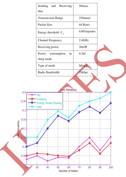
Table 1. Simulation Parameters

Parameters Value

Number of Nodes 50-100

Network Area 100 X 100

Sensing Range 16m

Initial Energy of sensor

node

(8)

584 |

P a g e

Sending and Receiving

Slot

50msec

Transmission Range 250meter

Packet Size 64 Bytes

Energy threshold E_th 0.001mjoules

Channel Frequency 2.4GHz

Receiving power 36mW

Power consumption in

sleep mode

0.36J

Type of mode Mica 2

Radio Bandwidth 76kbps

20 30 40 50 60 70 80 90 100

0 0.05 0.1 0.15 0.2 0.25 0.3 0.35

0.4 Link Reliability

Number of Nodes

L

in

k

R

e

li

a

b

il

it

y

DD Flooding

Energy Aware Routing LRR

Figure 1: Average Delivery Rate with various Transmission Rate

The average delay means the average delay between the instant the source sends a packet and moment the

destination receives this packet. When the transmission rate is 1 packet per second, we can see that the average

(9)

585 |

P a g e

In the proposed protocol, when the packets reach at destination, the relay or intermediate nodes have a lower

multiple strategies. In the forwarding node selection game, the probability that a great amount of packets are

forwarded by the same node is relatively low. Thus, the average delivery delay of our protocol does not

significantly increase with an increase in transmission rate. The following table 2 shows the network life time of

nodes in the respective routing protocols.

Routing

Protocols

Nodes Alive

Number of Nodes

100 Rounds

700 Rounds

20 Nodes 100 Nodes

LRR

(Proposed)

100

45

0.15

0.4 Flooding

59

18

0.05

0.07 DD

42

5

0.035

0.15 Energy

Aware

68

20

0.1

0.34 VI. CONCLUSION

In this paper, we introduce a zero-sum game theory for maintaining a sensor network lifetime. In this network

connectivity of nodes forward to any packets to its neighbor nodes. Zero-sum game theory improves the

network lifetime. Direct diffusion (DD) protocol, after 400 rounds, about 25% of nodes alive. In proposed link

reliability routing (LRR) protocol, after 550 rounds Network lifetime is increasing about 70%. Path reliability

for direct diffusion (DD) protocol is random. Path reliability for proposed link reliability routing (LRR)

protocol, increases Number of nodes increases to above 70 nodes, the path reliability is more than 0.3. This

shows that our proposed model and algorithm increases the network lifetime. Also, we will be optimizing the

algorithm to find the maximum usefulness function of all nodes that cooperate in path.

REFERENCES

[1] F.Akyldiz, W.Su, Y. Subramanian, Sankaras and E. Cayirci, “Wireless sensor networks: a survey”

Computer Networks,

[2] Vol.38, Pp. 393-422, 2002.

[3] “Theory of Games and Economic Behavior”-Von Neumann and Morgenstern-1953.

[4] “Game theory in Wireless sensor networks” – Pedro O.S.Vazdemelo, Cesar Fernandes, Raquel A.F, Mini

(10)

586 |

P a g e

[5] A.F.Loureiro.

[6] A. Agah, S. K. Das, and K. B.Basu, “Preventing DoS attack in sensor and actor networks: A game theoretic

approach”,

[7] IEEE Int’l. Conf. On Communications (ICC), Seoul, Korea, May 2005, pp. 3218-3222.

[8] S. Buchegger and J. Le Boudec, “Performance Analysis of the CONFIDANT Protocol,” Proc. Third

ACM Int’l

[9] Symp. Mobile AdHoc Networking & Computing, pp. 226-236, 2002.

[10]L. Buttyan and J.P. Hubaux, “Nuggets: A Virtual Currency to Stimulate Cooperation in Self

organized Mobile

[11]Ad- Hoc Networks, “Technical Report DSC/2001/001, Swiss Fed. Inst. Of Technology, Jan. 2001.

[12]7.W. Wang, M. Chatterjee, and K. Kwiat, “Enforcing Cooperation in Ad Hoc Networks with

Unreliable Channel,”

[13]Proc. Fifth IEEE Int’ Conf. Mobile Ad-Hoc and Sensor Systems (MASS), pp. 456-462, 2008.

[14]V. Srinivasan, P. Nuggehalli, C. Chiasserini, and R. Rao,“Cooperation in Wireless Ad Hoc Networks,”

Proc.

[15]IEEEINFOCOM, vol. 2, pp. 808-817, Apr. 2003.

[16]Chang, C.Y.; Shih, K.P.; Lee, S.C.; Chang, S.W. RGP: Active route guiding protocol for wireless sensor

networks with

[17]Obstacles. In Proceedings of IEEE MASS, Vancouver, Canada, October 2006; pp. 367-376.

[18]K. Sanzgiri, B. Dahill, B.N. L E.M. Royer, “A Secure Rohoc Networks”, In Proc. of on Network Protocols

(IC2002,