Improved multiobjective salp swarm
optimization for virtual machine placement
in cloud computing
Shayem Saleh Alresheedi
1, Songfeng Lu
1,2*, Mohamed Abd Elaziz
1,3and Ahmed A. Ewees
4,5Abstract
In data center companies, cloud computing can host multiple types of heterogene-ous virtual machines (VMs) and provide many features, including flexibility, security, support, and even better maintenance than traditional centers. However, some issues need to be considered, such as the optimization of energy usage, utilization of resources, reduction of time consumption, and optimization of virtual machine placement. Therefore, this paper proposes an alternative multiobjective optimization (MOP) approach that combines the salp swarm and sine-cosine algorithms (MOS-SASCA) to determine a suitable solution for virtual machine placement (VMP). The objectives of the proposed MOSSASCA are to maximize mean time before a host shutdown (MTBHS), to reduce power consumption, and to minimize service level agreement violations (SLAVs). The proposed method improves the salp swarm and the sine-cosine algorithms using an MOP technique. The SCA works by using a local search approach to improve the performance of traditional SSA by avoiding trapping in a local optimal solution and by increasing convergence speed. To evaluate the quality of MOSSASCA, we perform a series of experiments using different numbers of VMs and physical machines. The results of MOSSASCA are compared with well-known meth-ods, including the nondominated sorting genetic algorithm (NSGA-II), multiobjective particle swarm optimization (MOPSO), a multiobjective evolutionary algorithm with decomposition (MOEAD), and a multiobjective sine-cosine algorithm (MOSCA). The results reveal that MOSSASCA outperforms the compared methods in terms of solving MOP problems and achieving the three objectives. Compared with the other methods, MOSSASCA exhibits a better ability to reduce power consumption and SLAVs while increasing MTBHS. The main differences in terms of power consumption between the MOSCA, MOPSO, MOEAD, and NSGA-II and the MOSSASCA are 0.53, 1.31, 1.36, and 1.44, respectively. Additionally, the MOSSASCA has higher MTBHS value than MOSCA, MOPSO, MOEAD, and NSGA-II by 362.49, 274.70, 585.73 and 672.94, respectively, and the proposed method has lower SLAV values than MOPSO, MOEAD, and NSGA-II by 0.41, 0.28, and 1.27, respectively.
Keywords: Cloud computing, Virtual machine placement, Multiobjective optimization, Salp swarm algorithm, Sine-Cosine algorithm
Open Access
© The Author(s) 2019. This article is distributed under the terms of the Creative Commons Attribution 4.0 International License (http://creat iveco mmons .org/licen ses/by/4.0/), which permits unrestricted use, distribution, and reproduction in any medium, provided you give appropriate credit to the original author(s) and the source, provide a link to the Creative Commons license, and indicate if changes were made.
RESEARCH
*Correspondence: [email protected]
1 School of Computer
Introduction
Currently, the evolution and spread of technology double the quantity of data several times every minute; therefore, traditional data centers, which store these data locally, do not work as efficiently as before and have become unsuitable for many companies. Thus, traditional data centers should be improved to overcome several issues, including high maintenance costs, wasted floor space, high energy consumption, security, and high human resource costs. In addition, quality of service (QoS) requires companies to intro-duce high-quality services for their clients, including sending tasks to resources, task scheduling, and output satisfying results in an appropriate amount of time [1]. These problems can be approached by cloud computing servers.
Cloud computing can help the owners of datacenters overcome several issues through its flexibility, security, high scalability, QoS, and improved maintenance and support [1]. Cloud computing has the ability to host multiple types of heterogeneous servers; these servers host thousands of virtual machines (VMs); and each machine is provided with suitable resources (e.g., CPU, RAM, and storage) to be able to run all processes. Some cloud computing servers hold only one VM, while most servers host multiple VMs. This structure may cause overloading problems in some servers, which can reduce the perfor-mance of the servers and consume a large amount of energy [2].
VMs have also different workload types and resource specifications; thus, this may result in an imbalance in resource usage and high energy consumption [1]. Therefore, many issues need to be considered, such as the utilization of all resources, reduction of time consumption, and optimization of energy usage. The consumption of energy leads to increases in operating costs and it is related to resource utilization in datacent-ers. In this context, the energy cost of Amazon’s datacenters consumed more than 40% of its total operating costs [3]. In addition, the increase in energy consumption causes an increase carbon dioxide emissions and ecological problems [3]. Therefore, if energy consumption is reduced, the operating costs of datacenters will be reduced. An effec-tive technique to achieve this goal is to apply and optimize the VM placement (VMP) process [4].
VMP relates to the allocation of VMs to a relevant physical machine (PM). This pro-cess is considered to be an important problem in managing datacenter resources. It should be done in real-time without large time consumption. If this process consumes more time, it will reduce its main benefits of being applied in a real environment. This research topic has several optimization criteria that can be effective in achieving highly positive economic and ecological results. For this reason, resource allocation in cloud computing platforms has attracted increasing attention and has been widely studied by many researchers [5–8].
herd optimizer (SHO) [15] is another meta-heuristic that emulates selfish herd behavior. The SHO is used to solve global optimization problems [15], and there is another version of SHO that depends on the opposite-based learning method and that applied this algo-rithm to an optimization function [16]. The tree-seed algorithm (TSA) has been applied to address continuous optimization problems [17]. The TSA simulates the relationship between trees and their seeds. This algorithm has several applications: large-scale binary optimization [18], optimal power flow problem [19], and similarity and logic gate binary optimization [20].
Therefore, we introduce an alternative method called MOSSASCA to find a suitable solution for the VMP problem. MOSSASCA is a multiobjective salp swarm algorithm (SSA) using sine-cosine algorithms (SCAs) as local operators.
SSA is a recently developed optimization method that simulates the natural behav-ior of salp, barrel-shaped plankton (family Salpidae) that are mostly water by weight. In addition, they move in the same way as jellyfish. SSA was proposed to solve differ-ent kinds of optimization issues [21]. SCA is an evolutionary method proposed to pro-vide various solutions to different problems. It uses the mathematical model of sine and cosine functions and switches between them to obtain the optimal solution [22]. These methods were used in many previous studies and have shown good results [23–25].
The objectives of the proposed MOSSASCA are to maximize the mean time before a host shutdown, to reduce the power consumption and to minimize service level agree-ment violations (SLAVs). The proposed method starts by generating an integer popula-tion that represents solupopula-tions for the VMP and evaluates the quality of each solupopula-tion by computing the objective functions. Then, the nondominated (ND) solutions are deter-mined and saved in the archive. The next step uses the leader selection method to choose the best solution from the archive that is applied to update other solutions. Thereafter, the solutions in the current population are updated using the modified version of SSA, based on SCA. In MOSSASCA, the operators of SCA are used as local operators to improve the solutions of SSA and preventing them from becoming stuck at a local opti-mal point. All solutions updated by MOSSASCA are added to the archive. ND solutions are found and then are updated based on the size of the archive. The previous steps are executed until reaching stop conditions.
The rest of this study is organized as follows. “Related work” section lists the related works and problem formulation. “Background” secion describes the background of the methods used in this study. “Proposed MOSSASCA for VMP method” section explains the proposed method. The experiments and results are explained in “Results and discus-sion” section. The conclusion and future work are illustrated.
Related work
The techniques that can be applied to solve the problem of VMP resource allocation can be defined as multiobjective (MO) or single-objective. The process of finding the solution for more than one objective function simultaneously with different criteria is considered a multiobjective optimization problem (MOP).
Different types of meta-heuristic (MH) techniques are applied to solve the problem of single-objective VMPs. For example, Gabay et al. [33] applied first-fit decreasing, best-fit decreasing, and worst-fit techniques to locate destination PM for placing VMs. The authors reported that their proposed method is flexible, fast, and appropriate to be applied to real-life problems.
The authors of [34, 35] introduced simulated annealing (SA) algorithm-based VM con-solidation algorithm.
However, single-objective methods are not suitable in the case of balancing between different objectives; therefore, multiobjective (MOP) methods are used to find solutions that balance between the objectives.
MOP methods have been applied to different applications, such as restructuring traf-fic networks [36], data mining methods for knowledge discovery [37], multiple sequence alignment [38], wind turbine blade geometry design [39] and others [40, 41].
Several MOP methods have been proposed, including in [42], a multiobjective method based on the grasshopper optimization algorithm (GOA). This algorithm simulates the navigation behavior of grasshoppers in nature. The authors of [43] proposed an MO ver-sion of the ant lion optimizer (ALO) and applied it to solve engineering design problems. In [44], the multiobjective flower pollination algorithm is proposed, which simulates the behavior of plant flowers’ proliferation role. For finding solutions for constrained MOP problems, a modified water cycle algorithm has been proposed [45].
With all of this attention on MOP methods, minimal efforts have been exerted toward the optimization of multiobjective VMP problems by MH and hybrid-heuristic algo-rithms. For example, the authors of [2] applied biogeography-based optimization (BBO) as an optimization method in order to determine a solution for the VMP problem con-sidering server loads, inter-VMs, power consumption, resource wastage, and storage network traffic. In addition, the authors of [3] introduced a hybrid genetic algorithm (GA) to solve the VMP problem in a communication network and PMs in a data center. Gao et al. [46] proposed an MO ant colony optimization (ACO) algorithm to deal with VMP issues; it was applied to determine efficient ND solutions that minimize power consumption and resource usage. Other studies proposed intelligent models to decrease the power consumption in a cloud environment such as [47–51].
However, these models suffer from slow convergence and become stuck in local optima. In addition, the no free lunch (NFL) theorem [52] assumes that the optimization method does not have the ability to solve all problems with the same quality. Therefore, this consideration motivated us to propose an alternative multiobjective VMP method that can overcome the limitations of other methods.
based on SSA for practical considerations in radial distribution systems that determine optimal conductor and hosting capacity. For the fractional order proportional-integral-derivative (FOPID) controller problem, the SSA is used [59]. In [60], the authors presented an alternative job shop scheduling problem, whereas [61] presented training neural net-works using SCA for improving pattern classification.
In general, the contributions of this study can be formulated as follows:
– Proposing an alternative optimization approach that uses the multiobjective optimiza-tion concept to enhance the properties of SSA based on SCA as a local search.
– Applying the MOSSASCA method to solve the problem of VMP and allocating resources in cloud computing platforms.
Background
Problem formulation of VMP
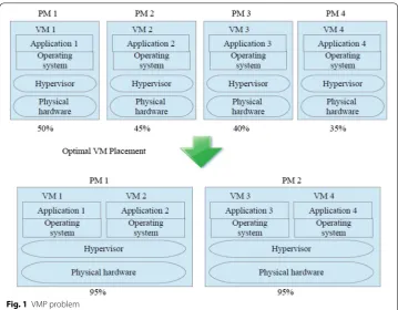
Physical cloud computing structures consist of many PMs. They contain the physical layers, or infrastructure, of cloud computing and they contain many components such as storage, RAM, CPUs, GPUs, and network connectors [8]. Therefore, cloud computing would not work without PMs. Each PM contains multiple VMs, where each VM can run an independ-ent operating system (OS) and applications. VMs require many resources include CPU time, memory space, and storage. Therefore, a VM obtains these resources from its PM. Figure 1 illustrates the VMP problem.
Figure 1 contains four servers that run four VMs. Four virtualized applications are hosted on the system. The following points describe the process of VMP.
1. For each PM, calculate the requirement of the application’s resource through the sta-tistics of the usage of the server’s resource in a period of time.
2. Select a proper PM with the comparable type of CPU, compatible software, storage, and similar network properties.
3. Assign VM1 to the PM1 in step 2, and assign VM2 to the PM1 if it has sufficient
resources.
4. Repeat this mechanism until each VM is assigned to a suitable PM and, if required, add a new PM to build the structure of a server farm.
The following subsections describe the PMs, VMs, constraints, and objective function.
Physical machine
The PMs consist of more than one machine, and all these machines have physical layers, as shown in the following equation:
where NP describes the total number of PMs. Each PM has the following:
where PMi,(i=1, 2,. . .,NP) defines the number of the current PMs. PMipmax is the maximum power consumption of the ith PM in units of [W]. The PMCPUi ,PMiram and PMhddi are the processing resources (in [ECU]), the memory resources (in [GB]), and the storage resources (in [GB]) of the PMi.
Virtual machine
The VMs consist of one or more VMs, as shown in the following equation:
where NV describes the total number of VMs. Each VM has the following resources:
where j is the current VM’s number. VMjCPU,VMjram , and VMjhdd represent the process-ing, memory, and the storage requirements of the jth VM, respectively.
Objective functions
In this section, the three objective functions are defined below:
– Energy consumption: The servers consume a large volume of power when they are in an idle state.
(1) PM= [PM1,PM2,PM3,. . .,PMNP],
(2)
PMi=(PMiCPU,PMiram,PMihdd,PM pmax i ),
(3) VM= [VM1,VM2,VM3,. . .,VMNV],
(4) VMj=(VMjCPU,VMjram,VMjhdd), j=1, 2,. . .,NV,
(5) fEnergy=
NV
i=1
((PMipmax−PMipmin)×UCPUi(g)+PM
pmin
where fEnergy represents the total power consumption of the PMs, while
PMpmini =PMipmax×0.6 [62, 63] defines the minimum power consumption of PMi .
UCPUi(g) represents the utilization ratio of resource utilized by PMi at instant t, while Yi(g)∈ [0, 1] is equal to 1 if the PMi is turned on; otherwise, Yi(g)=0.
– SLAV: The infrastructure of cloud computing and hosts try to meet QoS require-ments, which are modeled in the SLAV form to maximum response time or mini-mum throughput. SLAV can be caused by a host, as defined in the following equa-tions.
where SLAO represents the average ratio of the period in the case the host experi-ences CPU utilization of 100% and is defined as follows:
where Tai is the active time of i-th host, and Tsi represents the total time when the i -th host experiences 100% SLAV utilization. Moreover, -the SLAM represents the deg-radation in the performance due to the migration of VMs and is defined as follows:
where Crj indicates the total CPU utilization needed by the VMj , and Cdj represents the degradation in the performance that results from VM migration.
– Mean time before a host shutdown (MTBHS): This time is measured in seconds, and the average is calculated as follows.
where hi represents the host shutdown time.
Constraints:
(6) fSLAV =SLAO×SLAM,
(7)
SLAO= 1
NP NP
i=1
Tsi Tai
,
(8)
SLAM= 1 NV
NV
j=1
Cdj
Crj ,
(9)
fjMTBHS = 1 NP
NP
i=1
hi,
(10) NP
i=1
Bji(g)≤1∀j∈ {1,. . .,NV},
(11)
NP
i=1
VMcpuj ×Bji(g)≤PMCPUi,
(12) NP
i=1
where Bji=1 when the VMj allocates on PMi ; otherwise Bji=0 . In constraint (10), VMi
should be executed on a single PMj and when its SLAVi is lowest priority (in this work, s = 2). Here, it should not allocated to any PM. In constraints (11)–(13), the current PM ( PMj ) must have sufficient resources to be able to work properly and serve all its VMs at
instant t.
Multiobjective optimization
The MOP problems are optimization problems that need solutions with more than one objective function [64]. However, this kind of problem is considered to be an NP hard prob-lem because it contains a set of conflicting objectives. In general, the MOP is given as [64]:
where fm(x) and Ω are the m-th of the objective function and of the search domain,
respectively. The Lj and Uj are lower and upper boundaries of i-th solution, respec-tively. The inequality and the equality constraints are represented by Gj(x) and hj(x) ,
respectively.
To find the optimal solution that balances all conflicting objective functions, we use the concept in MOPs known as Pareto optimal dominance. Based on this concept, we consider that the solution x has better results than another solution y if (and only if) it has objective function values better than the other objective values of (y). This can be formulated as
Therefore, the solution x that satisfied Eq. (17) is said to dominate y.
From the previous definition of the dominated solution, there exists a set of tions called Pareto optimal (PF; also called nondominated solutions) where no solu-tion can dominate them. The set of all PF solusolu-tions is represented as follows:
In addition, the values of the solutions that belong to the Pareto set in the objective domain is called Pareto front and represented as follows:
Salp swarm algorithm
Salp swarm algorithm (SSA) is a new meta-heuristic method, introduced by [21]. SSA emulates the behavior of salps of the family Salpidae. They move like jellyfish, and a high percentage of their weight is water [65]. The working mechanism of SSA starts by producing a random set of NS solutions (X) with dimension D. The X is split into
two sets based on the location of salps in the population. A salp in front of the food (13)
NP
i=1
VMhddj×PMji(g)≤PMhddi,
(14)
min f(x)= [f1(x),. . .,fM(x)], x = [x1,. . .xn] ∈Ω,
(15) subject to:hj(x)=0, j=1, 2,. . .,Nh,
(16)
Gl(x)≥0, (l=1, 2,. . .,NG),
(17) ∀j:fj(x)≤fj(y)and∃i:fi(x) <fi(y).
(18) Pareto set= {x|x∈Ωand x is Pareto optimal}.
chain will be in the leader group; the rest will be in the followers’ group. The leader group x1 states the solution to the problem. It is updated using the following Eq. [21]:
where x1j(g) and xbj(g) define the leader’s position and the food source in the j-th
dimen-sion at iteration g, respectively. ubj and lbj define the upper and lower bounds of
dimen-sion j, respectively. α2 and α3 represent random values in [0, 1] that maintain the search space [21]. To give balance to the exploitation and exploration phases, the α1 is updated at each iteration g depending on the maximum number of iterations gmax as follows [21]:
Then, the position of the followers’ solution xi is updated using Eq. (22) [21]:
Algorithm 1 shows all steps of the SSA [21].
Algorithm 1steps of SSA
1: Produce a random set ofNS solutionsX.
2: while(g < gmax)do
3: For each solution compute its objective functions. 4: Define the leader (xb).
5: Calculater1with Eq. (21)
6: foreach solutionxi, i= 1, ..., NSdo
7: if (i== 1)then
8: Use Eq. (20) to update the leader’s position or 9: else
10: Use Eq. (22) to update the followers’ position. 11: end if
12: end for 13: end while
14: Output the leader position (xb).
Sine‑cosine algorithm
The sine-cosine algorithm (SCA), presented by [22], is based on the mathematical model of the sine and cosine functions to improve its population and obtain the solution for the problem. It switches between these models to achieve the best result.
The working mechanism of SCA begins by randomly producing an initial set of NS
solutions X with D dimensions. Afterward, for each solution, it calculates the fitness val-ues. The solution with the best fitness value ( fb ) is considered as the best solution ( xb ).
The xb and the parameters βi,i=1, 2, 3, 4 are used to update the solutions as in Eq. (25). SCA repeats these steps until the stop condition is met, shown in Algorithm 2.
SCA updates its population using the sine function as follows [22]:
and updates its population using the cosine function as follows [22]:
(20)
x1j(g+1)=
xbj(g)+α1((ubj−lbj)×α2+lbj) α3≤0,
xbj(g)−α1((ubj−lbj)×α2+lbj) α3>0,
(21)
α1=2e − 4g
gmax 2
,
(22)
xij(g+1)= 1
2(x
i
j(g)+xi−
1
j (g)), i=2,. . .,NS
(23) xi(g+1)=xi(g)+β1×sin(β2)× |β3xb(g)−xi(g)|
The SCA uses a parameter β4 to switch between these equations as shown in the follow-ing [22]:
where |.|, xb(g) , and xi(g) define the absolute value, the target and the current solu-tions at iteration g, respectively. The βi,i=1, 2, 3, 4 represent random variables of [0, 1] [22]. β2 defines the path of the next solution’s movement either toward or away from xb .
β3 represents a random number that adds weight to xb to check whether it
stochasti-cally preserves (when β3>1 ) or ( β3<1 ) the influence of desalination upon finding the domain. β1 is applied to switch between exploration and exploitation in order to define the optimal part for the next solution. This part may be higher than the upper bound or lower than the lower bound, Thus, it is updated as follows [22]:
where g, σ , and gmax define the current iteration, a constant, and the iterations number,
respectively.
Algorithm 2The steps of SCA 1: Produce a set of solutionsX. 2: while(g < gmax)do
3: Compute the fitness valueffor each solution.
4: Definexbthat has the best fitness valuefb.
5: Updateβ1, β2, β3,andβ4values. 6: Use Eq. (25) to updateX. 7: end while
8: Outputxb.
Proposed MOSSASCA for VMP method
The section discusses the main steps of the multiobjective VM placement method that combines the improvement of the behavior of the SSA using the SCA. Therefore, the proposed method is called MOSSASCA. The goal of the proposed method is to search for the optimal set of approximate Pareto front (PF), which represents the optimal solu-tions for minimizing SLAV, reducing power consumption and maximizing time before a host shutdown [as shown in Eqs. (5)–(9)].
In general, the proposed MOSSASCA begins by receiving the parameters (i.e., the number of VMs ( NV ), the number of hosts ( NP ), the number of solutions ( NS ), and the max number of iterations. Afterwards, the next steps are to generate a random popula-tion that contains a set of solupopula-tions, each of which represents the index of VM. Subse-quently, the performance of each solution is measured by computing objective functions, and the best solution is selected using concepts of dominance. Therefore, each solution is changed and updated by the SSASCA, where SCA is applied to improve the SSA by working as a local search technique. The nondominated (ND) solutions in the archive are updated by comparing them with the ND solutions from the updated population. This sequence is executed until reaching a maximum number of iterations.
(25) xi(g+1)=
xi(g)+β1×sin(β2)× |β3xb(g)−xi(g)| if β4<0.5 xi(g)+β1×cos(β2)× |β3xb(g)−xi(g)| if β4≥0.5
(26)
β1=σ−g σ
gmax
The previously mentioned steps of the proposed MOSSASCA can be classified into three phases: (1) initialization, (2) updating the population using SSASCA, and (3) updating the archive of ND solutions. These phases are discussed in detail in the follow-ing subsections.
Initialization
In this phase, the MOSSASCA starts by initializing a set of NS solutions X where the
value of each solution Xi,(i=1, 2,. . .,NS) form the index of the VM and the dimension equal to the total number of VMs ( NV ). The solution is generated using the following
equation:
where NP represents the number of PMs, LP is the minimum number of PMs (set to
one), and floor is a function used to convert the real number to an integer value. To clarify this definition, we consider the NP =5 , and NV =8 , then Xi= [2 5 3 3 3 1 2 4] . This representation means that the first and seventh VMs are allocated to the second PM and the second VM is allocated to the fifth PM. The third to fifth VMs are allocated to the third PM, and the sixth and eighth VMs are allocated at the first and fourth PMs, respectively.
The next step is that the objective function is calculated for each solution using the fol-lowing equation:
where fSLAV,fEnergy , and fMTBHS are defined in Eqs. (5)–(9). Thereafter, the ND
solu-tions are allocated and are stored in archive AR.
Algorithm 3Initialization Stage
1: Putt= 0, archiveAR= [] 2: fori= 1 toNdo
3: GenerateXijusing Equation (27).
4: Compute the objective function forxiusing Equation (28).
5: end for
6: Update the ND solutions inAR.
Update the population using SSASCA
In this phase, the solutions X are updated by using the hybrid SSA and SCA. The aim of using the SCA algorithm is to give the SSA the capability of skipping the local point. The hybrid SSASCA algorithm starts by determining the best solution. However, this process is different from the single-objective optimization, where each solution has only one function. That in MOP has more than two objective values. Therefore, the leader selection mechanism (LSM) is applied to the nondominated solutions in archive AR (see [66] for more details) to select the best solution ( Xb ). The LSM uses the roulette-wheel method to choose Xb based on the probability ( ProbSel ), which is computed as follows:
where Nsegi represents the number Pareto optimal solutions of the crowded segment i,
while C>1 is a constant number.
(27) Xij=floor(LP+rand×(NP−LP)), j=1,. . .,NV
(28) Min F= [fEnergy;fSLAV;fMeantime]T,
(29)
Therefore, to switch between SSA and SCA, we compute the probability (Pr) of the power fitness function as follows:
If the current solution has Pri ≥η ( η∈ [0, 1] ), then the SSA is used to update Xi ; other-wise, the SCA is used to update Xi . The next step is to convert the updated solution into an integer solution using the floor function (i.e., Xi=floor(Xi) ); then, the objective
func-tions are calculated for each solution.
Algorithm 4Update stage
1: Determinexbusing the leader selection method (LSM) using Equation (29). 2: fori= 1 toNdo
3: Calculate theP rivalue ofXi. 4: if(P ri≤η)then
5: Use Equation (25) to updateXi,
6: else
7: if i≤N/2then
8: Use Equation (20) to updateXi(leader), 9: else
10: Use Equation (22) to updateXi(follower). 11: end if
12: end if
13: end for
Update the archive
This stage begins by combining the current population with the archive AR, followed by the determination of ND solutions. This process is critical to improve convergence to the true PF and preserve the population’s diversity by using the density estimation informa-tion [67–70].
In general, the archive AR is updated by comparing its ND solutions with each solu-tion in the populasolu-tion (i.e., Xi ∈X ) using the Pareto dominance concepts. Here, the solution Xi will swap any solution XA in AR when Xi dominates XA , and if there is a set
of solutions in AR is dominated by Xi , then this set will be removed from AR, and Xi will be added to AR. However, if Xi must be added to AR and the size of AR is full, then the crowded segment method is used. The segmentation of the objective space is rearranged by using the grid mechanism, and the most crowded segment is determined to delete the solution from AR. Thereafter, the Xi will be combined with the least crowded segment to improve the PF’s diversity. In addition, solution Xi is not appended to AR when any solu-tion dominates it (i.e., Xi ) [71]. The final step in this phase is to enhance the population X by selecting the best NS solutions from AR.
Algorithm 5Stage of Updating ArchiveAR 1: In: UpdatedX,
2: AddXto the ND solution inAR. 3: Determine the ND solutions ofAR.
4: Check the size ofARand choose only the bestNS ND solutions.
5: Return: ArchiveAR.
(30) Pri=
f1
NS
Full description of MOSSASCA method
The remaining parts of the proposed MOSSASCA method for VMP are presented in Algorithm 6. Here, the current generation is represented by g and the maximum num-ber of iterations is given by gmax . The proposed MOSSASCA starts by determining the
input to the initialization phase (as described in Algorithm 3) and receiving the output (i.e., population X and archive AR) from it. The next step is to update X based on the hybrid SSASCA algorithm (as described in 4). Then, Algorithm 5 is used to find the NDS and update AR. The steps of two algorithms (i.e., Algorithm 4, Algorithm 5) are repeated until the terminal conditions are satisfied.
Algorithm 6 Multiobjective salp swarm algorithm based on sine-cosine algorithm (MOSSASCA).
1: Input: number of VMs and PMs, population sizeNS, and maximum number of generationsgmax
2: Output: nondominated solutions saved in archiveAR.
3: Use Algorithm 3 to generate the populationX.
4: repeat
5: Use Algorithm 4 to update the solutions.
6: Use Algorithm 5 to update the nondominated solutions saved in archiveARand update the
populationX.
7: g=g+ 1
8: untilg <=gmax.
Complexity of MOSSASCA method
The complexity of the MOSSASCA method depends on several items, for example, the dimension of the tested problem, the number of solutions NS , the number of objectives M, the maximum number of iterations tmax . Therefore, the complexity of MOSSASCA is
given by
where Nprob1 and Nprob1 represents the number of solutions updated using the SSA and SCA respectively. cof is the cost of objective function.
Results and discussion
A set of experiments are performed to assess the performance of the MOSSASCA as a multiobjective VMP method to find the optimal solution to the VM allocation problem. In addition, the results of MOSSASCA are compared with those of other approaches, such as NSGAII [72], MOEA-D [73], MOPSO [74], and MOSCA [75].
Environment description
In this section, the description of the environment is explained, where the CloudSim toolkit simulation framework is used to simulate the cloud computing environments [76]. The experimental setup used in this study simulates the real configurations of cloud computing infrastructure, which includes 160 IBM Server x3250 and Intel Xeon 3480 CPU, 160 IBM Server x3250 and Intel Xeon 3470 CPU model, 160 HP ProLiant ML110 (31)
O(MOSSASCA)=O(tmax(NV ×(NS×Nprob1+NS×Nprob2)
G3, 160 HP ProLiant ML110 G4, and 160 HP ProLiant ML110 G5. Table 1 shows a set of parameters used in the experiments for VM simulations.
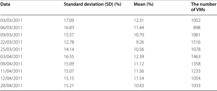
In addition, the workload data are extracted from the project of CoMon data [77, 78]. Statistical values of the utilization (shown in %) of data (daily) are given in Table 2.
The performance of the MOSSASCA is compared with other algorithms, such as NSGAII, MOEAD, MOPSO, and MOSCA. To evaluate the performance of these meth-ods, we use different numbers of VMs (25, 75, and 100) and hosts (50, 150, and 200), where 50 VMs are assigned to 25 hosts, 150 VMs are assigned to 75 hosts, and 200 VMs are assigned to 100 hosts.
All algorithms are implemented using jMetal java framework, which is installed on Windows 10 (64-bit).
Performance measures
The proposed method is evaluated on the basis of MOP performance measurements, including hypervolume (HV), spread (SP), generational distance (GD), epsilon (EPS), and inverted generational distance (IGD) [79].
1. HV: It is applied to evaluate the nearness and variety of PF by computing the area size dominated by its solutions. If the HV of X>B , then X Pareto optimal converges to be greater than B.
Table 1 The Parameters of VM simulation
Parameter Value
VM types 2, 4
VM RAM 870, 1740 MB
VM bandwidth 100 to 200 Mbit/s
VM MIPS 2500, 100
Number of VMs 50, 100, 150, 200
VM PES 1,1
Table 2 Properties of the workload
Data Standard deviation (SD) (%) Mean (%) The number of VMs
03/03/2011 17.09 12.31 1052
06/03/2011 16.83 11.44 898
09/03/2011 15.57 10.70 1061
22/03/2011 12.78 9.26 1516
25/03/2011 14.14 10.56 1078
03/04/2011 16.55 12.39 1463
09/04/2011 15.09 11.12 1358
11/04/2011 15.07 11.56 1233
12/04/2011 15.15 11.54 1054
2. SP: It is used to evaluate the extent of spread achieved between the solutions and compute the nonuniformity in the distribution of solutions, and it is defined as
where di represents the Euclidean distances between the set of solutions that have the mean value d¯ , and where de
i represents the distance between the extreme solu-tions and PF∗ . M and |Q| are the total number of objective functions and the num-ber of solutions in PF∗ , respectively. The smaller Spread value indicates that the algo-rithm is better than others.
3. GD: GD defines the average distance between the true Pareto front and the estimated front. Equation (34) defines this measure:
In Eq. (34), n= |fp| defines the number of elements of the ND solutions, and di defines the Euclidean between the closest front’s solution of Pareto optimal in the objective space and reference solution (RP).
4. IGD: It is applied to compute the nearness between the reference optimal solution (RP) and the archived Pareto solution. Equation (35) defines this measure:
The smaller IGD value indicates better performance.
5. EPS: It is used to find the minimum value where the approximation PF is mapped to the objective space that dominates the true PF.
where r and a are the solutions in the true PF and the approximate PF, respectively. The algorithm with the smallest EPS is considered to be the better one.
Experimental results analysis Comparison with other algorithms
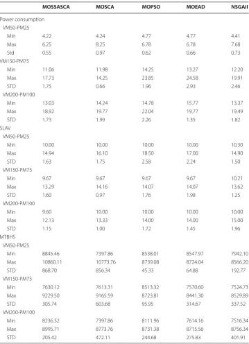
The comparison results between the MOSSASCA and the other algorithms in order to determine the optimal solution for the VMP in cloud computing are given in Table 3
and Figs. 2, 3, 4. The results show that the proposed MOSSASCA method performs bet-ter than the other methods. Specifically, the proposed method has lower minimum and maximum power consumption in all tested problems. The standard deviation of the (32) HV =volume
|PF|
�
i=1 ai
(33) Spread=
M
i=1dei +
|Q|
i=1|di− ¯d|
M
i=1diE+ |Q| ¯d
,
(34) GD(fp,fp∗)=
n
i=1d2i
n .
(35)
IGD=
r∈RPd
|RP| , d= ||a−r||2,∀a∈PF,r∀RP.
(36)
EPS=max
proposed method is smaller than all other methods except the MOEAD in the VM200-PM100 problem.
In addition, the minimum value of SLAV is achieved using the proposed method and by using the MOSCA, MOPSOA, and MOEAD algorithms in problems VM50-PM25 and VM150-PM75, but the proposed method achieves the best value in the VM200-PM100 problem. The proposed method has better maximum SLAV value than the other methods. However, the NSGA-II algorithm has the best standard deviation in problem
Table 3 The comparison of results among the algorithms in each tested VMP problem
MOSSASCA MOSCA MOPSO MOEAD NSGAII
Power consumption VM50-PM25
Min 4.22 4.24 4.77 4.77 4.41
Max 6.25 8.25 6.78 6.78 7.68
Std 0.55 0.97 0.62 0.66 0.73
VM150-PM75
Min 11.06 11.98 14.25 13.27 12.20
Max 17.73 14.25 23.85 24.58 19.91
STD 1.75 0.66 1.96 2.93 2.46
VM200-PM100
Min 13.03 14.24 14.78 15.77 13.37
Max 18.92 19.77 22.04 19.77 19.49
STD 1.73 1.99 2.26 1.35 1.82
SLAV VM50-PM25
Min 10.00 10.00 10.00 10.00 10.30
Max 14.94 16.10 18.50 17.00 14.90
STD 1.63 1.75 2.58 2.24 1.50
VM150-PM75
Min 9.67 9.67 9.67 9.67 10.21
Max 13.29 14.16 14.07 14.07 13.62
STD 1.60 0.97 1.76 1.98 1.25
VM200-PM100
Min 9.60 10.00 10.00 10.00 10.00
Max 12.13 13.33 14.00 14.00 15.00
STD 1.15 1.00 1.72 1.45 1.96
MTBHS VM50-PM25
Min 8845.46 7397.86 8538.01 8547.97 7942.10
Max 10860.11 10773.76 8739.08 8724.04 8566.20
STD 868.70 856.34 45.33 64.88 192.77
VM150-PM75
Min 7630.12 7613.31 8513.32 7570.60 7524.73
Max 9229.50 9165.59 8723.81 8441.30 8529.89
STD 305.74 603.68 95.95 314.67 337.52
VM200-PM100
Min 8236.32 7397.86 8111.96 7614.16 7516.34
Max 8995.71 8773.76 8731.38 8715.56 8756.34
VM50-PM25, and the MOSCA method has better value in problems VM150-PM75 and VM200-PM100.
The best maximum and minimum MTBHS values are achieved by the MOSSASCA in all the tested problems, but the best standard deviation is achieved by MOPSO in problems VM50-PM25 and VM150-PM75. Furthermore, the proposed method has the smaller standard deviation value in the VM200-PM100 problem.
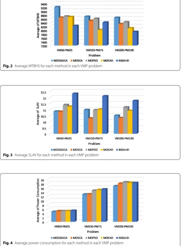
Figures 2, 3, and 4 show the average time, SLAV, and energy, respectively. The fig-ures show that the proposed method provides lower average power consumption and
Fig. 2 Average MTBHS for each method in each VMP problem
Fig. 3 Average SLAV for each method in each VMP problem
SLAV values than the other methods in each tested problem. The methods have simi-lar performance in VM50-PM25, but MOPOS and NSGA-II have the worst value in VM200-PM100 and VM150-PM75, respectively. Power consumption is increased as the numbers of PMs and VMs are increased. The proposed method and MOSCA nearly have the same SLAV value in VM50-PM25, but the proposed method produces better results than all other methods in the other two problems. Among the methods, NSGA-II has the worst results in three problems, whereas MOSCA, MOPSO, and MOEAD have nearly the same average value of SLAV in the VM150-PM75 problem. However, MOSCA has better results than MOPSO and MOEAD in the VM200-PM100 problem. Moreover, the worst MTBHS value is achieved by NSGA-II in problems VM50-PM25 and VM200-PM100, and MOEAD in VM150-VM75. The MOSSASCA shows best value among all tested algorithms in each tested problem. These results suggest that MOS-SASCA provides maximum utilization of each resource.
Performance evaluation based on MOP indicators
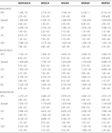
To investigate the quality of PFs obtained by each method we evaluate a set of MOP indicators given in Table 4 for each tested problem. From this table, it can be noted that the MOSSASCA performs better than the other methods in approximating PFs. For example, in terms of EP, HV, and IGD, the MOSSASCA ranks first of in all tested prob-lems. However, in terms of spread, MOSCA ranks first in testing problems in the VM50-PM25 and VM150-PM75, followed by the proposed MOSSASCA method, which has a smaller GD value in the third problem (i.e., VM200-PM100). MOSSASCA has a smaller GD value only in problem VM50-PM25, but MOPSO has a smaller GD value in two other problems. In addition, we can conclude from the table that MOEAD and NSGA-II generally have the worst performance in the tested problems.
From all the previous results, it can be concluded that the MOSSASCA outperforms the other methods based on the MOP indicators.
Influence the parameters of proposed method
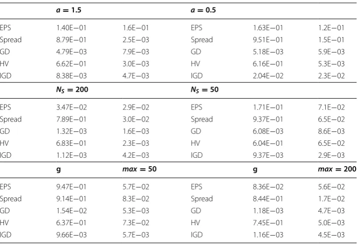
In this experiment, we investigate the influence of different parameters on the perfor-mance of the MOSSASCA. Table 5 illustrates the results of the proposed MOSSASCA based on different values of a= [1, 4] , NS=[50, 200], and gmax=[50, 200]. The proposed
method at a=1.5 is better than that at a=0.5 , indicating that the performance of the MOSSASCA increases with increasing a. In addition, population size affects the perfor-mance of MOSSASCA. Specifically, the MOSSASCA performs better at pop=200 than at pop=50 and pop=100 as in Table 4. Moreover, similarly, the performance of SASCA is affected by the number of iterations, and the results showed that the MOS-SASCA achieves high performance at iter=200.
Influences of VMs and PMs on the proposed method
result with VM200-PM500. In VM400-PM1000, the EPS of the MOSSASCA is the larg-est among the three problems. Based on the spread measure, the quality of the MOS-SASCA in the three problems is nearly the same; however, the best value is achieved in VM200-PM500. The same observation is found for the values of GD, where the value of the MOSSASCA at VM200-PM500 is better than its value in the other prob-lems. In addition, the HV value of the MOSSASCA at VM400-PM100 is better than in other problems. In addition, it can be observed that the best IGD value is achieved when MOSSASCA is used to solve the VM300-PM600. From these experimental series, it can be observed that the performance of MOSSASCA, in terms of MOP indicators, is not largely notable when solving the VM problem with VMs of 200–400 and PMs of 500–1000.
Table 4 Comparison results based on MOP indicators
MOSSASCA MOSCA NSGAII MOEAD MOPSO
VM50-PM25
EPS 1.54E−01 2.77E−01 7.14E−01 6.12E−1 6.12E−01
2.2E−02 2.5E−02 2.3E−04 0.00 0.0E+00
Spread 1.36E+00 4.10E−01 1.08E+00 1.30E+00 1.05E+00
2.6E−02 1.3E−01 2.3E−04 6.0E−02 2.9E−03
GD 4.29E−03 4.73E−02 1.58E−01 3.54E−02 3.48E−02
1.4E−03 2.2E−02 7.1E−05 1.1E−04 1.1E−06
HV 4.91E−01 4.16E−01 2.31E−01 3.36E−01 3.36E−01
1.5E−02 1.9E−02 1.7E−04 1.3E−04 2.6E−08
IGD 1.08E−03 2.77E−03 1.42E−02 1.33E−02 1.35E−02
7.8E−05 4.6E−04 1.6E−06 1.6E−05 2.1E−05
VM150-PM75
EPS 1.16E−01 1.95E−01 4.43E−01 3.40E−01 2.40E−01
8.3E−02 5.1E−02 9.2E−05 2.2E−04 0.0E+00
Spread 1.50E+00 7.79E−01 1.01E+00 1.27E+00 9.08E−01
9.1E−02 8.2E−02 2.0E−02 5.7E−02 5.2E−02
GD 1.93E−03 1.31E−02 1.22E−02 7.15E−03 9.99E−05
3.1E−04 7.3E−03 1.9E−04 3.8E−04 1.4E−04
HV 6.79E−01 6.15E−01 4.53E−01 5.40E−01 6.33E−01
2.8E−03 4.8E−03 8.1E−05 9.9E−03 1.1E−07
I GD 1.22E−03 2.46E−03 8.73E−03 7.44E−03 7.79E−03
8.7E−04 7.2E−05 3.9E−05 1.6E−04 1.0E−04
VM200-PM100
EPS 1.27E−01 4.58E−01 3.97E−01 3.46E−01 2.91E−01
3.8E−03 5.8E−04 1.5E−04 9.4E−03 6.8E−02
Spread 7.35E−01 1.17E+00 1.07E+00 1.16E+00 1.14E+00
2.6E−02 1.2E−04 2.0E−02 9.9E−02 5.0E−03
GD 3.90E−02 4.61E−02 6.65E−03 3.50E−03 1.08E−04
2.8E−03 1.30E−03 3.6E−04 1.6E−03 9.8E−05
HV 6.10E−01 6.68E−01 4.76E−01 5.34E−01 7.00E−01
1.1E−03 8.1E−03 1.4E−04 1.7E−02 5.1E−02
IGD 5.55E−03 7.1E−03 1.18E−02 1.10E−02 1.10E−02
From all the previous experimental results, it can be noted that the performance of MOSSASCA is better than the other methods in terms of the three objectives functions and the performance measurements. This performance results from the high skill of the SSA in exploration of the search domain and in using the operators of the SCA algo-rithm to improve the exploitation ability of the SSA through working as a local search method. Additionally, this leads to finding the nondominated solution that best balances among the three objectives of solving the VMP problem in cloud computing. Moreover, it can be noted that the performance of the other multiobjective VMP methods was less than that of the proposed method in this study and that the quality of the algorithms was not fixed when changing the problems. This outcome is because each algorithm has a different ability regarding either the exploration or exploitation of the search domain. However, there are some limitations for MOSSASCA, such as the fact that its computa-tional time will require addicomputa-tional improvement to make it more suitable for real-time VMP problems.
Table 5 Results of MOP indicators under different parameter values in the proposed method
a=1.5 a=0.5
EPS 1.40E−01 1.6E−01 EPS 1.63E−01 1.2E−01
Spread 8.79E−01 2.5E−03 Spread 9.51E−01 1.5E−01
GD 4.79E−03 7.9E−03 GD 5.18E−03 5.9E−03
HV 6.62E−01 3.0E−03 HV 6.16E−01 5.3E−03
IGD 8.38E−03 4.7E−03 IGD 2.04E−02 2.3E−02
NS=200 NS=50
EPS 3.47E−02 2.9E−02 EPS 1.71E−01 7.1E−02
Spread 7.89E−01 3.0E−02 Spread 9.37E−01 6.5E−02
GD 1.32E−03 1.6E−03 GD 6.08E−03 8.6E−03
HV 6.83E−01 2.3E−03 HV 6.04E−01 6.5E−02
IGD 1.12E−03 4.2E−03 IGD 9.37E−03 2.9E−03
g max=50 g max=200
EPS 9.47E−01 5.7E−02 EPS 8.36E−02 5.6E−02
Spread 9.14E−01 8.3E−02 Spread 8.44E−01 1.7E−02
GD 1.54E−02 5.3E−03 GD 1.18E−03 4.7E−03
HV 6.37E−01 7.3E−02 HV 7.45E−01 5.0E−03
IGD 9.66E−03 5.7E−03 IGD 1.16E−03 4.5E−03
Table 6 Results of changing the number of VMs and PMs
Power
consumption SLVA MTBHS EPS Spread GD HV IGD
Conclusion
This paper proposes an alternative MOP method for finding the optimal solution to the VM consolidation problem. The main objectives of the proposed MOSSASCA are to maximize MTBHS, to reduce power consumption, and to minimize SLAV. MOSSASCA is proposed to find solutions that can minimize conflict between the three objectives. In MOSSASCA, the SCA is applied as a local search approach to enhance the perfor-mance of traditional SSAs by preventing them from getting stuck in a local optimal solution and increasing convergence speed. To assess the performance of the proposed method, we perform a set of experiments using different numbers of VMs and physi-cal machines. The results of MOSSASCA are compared with that of well-known MOP methods, including NSGA-II, MOPSO, and MOSCA. The experimental results show that MOSSASCA is better than others on the basis of MOP indicators and in achieving the three objectives. Here, the proposed method achieves the best results in three MOP indicators, namely, EPS, HV, and IGD. The MOSCA and MOPSO methods are better according to the value of spread and GD, respectively. Compared with the other meth-ods, MOSSASCA exhibits a better ability to reduce power consumption and SLAV while increasing MTBHS.
Given the superiority of the proposed MOSSASCA method, it can be extended to solve more than the three objectives in VM placement in cloud computing. It can also be applied to different fields, for example, feature selection, image segmentation and job scheduling.
Authors’ contributions
All authors contributed equally to this study. SSA collected and prepared the data; MAE and AAE implemented the proposed method; and SL and the other three authors wrote the main text and discussed the results. All authors read and approved the final manuscript.
Author details
1 School of Computer Science & Technology, Huazhong University of Science and Technology, Wuhan 430074, China. 2 Shenzhen Huazhong University of Science and Technology Research Institute, Shenzhen 518063, China. 3 Department
of Mathematics, Faculty of Science, Zagazig University, Zagazig, Egypt. 4 University of Bisha, Bisha, Kingdom of Saudi
Arabia. 5 Department of Computer, Damietta University, Damietta, Egypt.
Acknowledgements
This work is supported by the Science and Technology Program of Shenzhen of China under Grant Nos. JCYJ20180306124612893, JCYJ20170818160208570 and JCYJ20170307160458368.
Competing interests
The authors declare that they have no competing interests. Data availability statement
The data used to support the findings of this study are available from the corresponding author upon request. Funding
Not applicable.
Publisher’s Note
Springer Nature remains neutral with regard to jurisdictional claims in published maps and institutional affiliations.
Received: 20 October 2018 Accepted: 25 March 2019
References
1. Xu M, Tian W, Buyya R (2017) A survey on load balancing algorithms for virtual machines placement in cloud com-puting. Concurrency Comput Pract Exp 29(12):e4123
3. Tang M, Pan S (2015) A hybrid genetic algorithm for the energy-efficient virtual machine placement problem in data centers. Neural Process Lett 41(2):211–221
4. Fu X, Zhao Q, Wang J, Zhang L, Qiao L (2018) Energy-aware vm initial placement strategy based on bpso in cloud computing. Sci Program 2018:9471356
5. Bajo J, De la PF, Corchado JM, Rodríguez S (2016) A low-level resource allocation in an agent-based cloud comput-ing platform. Appl Softw Comput 48:716–728
6. Cao Z, Lin J, Wan C, Song Y, Zhang Y, Wang X (2017) Optimal cloud computing resource allocation for demand side management in smart grid. IEEE Trans Smart Grid 8(4):1943–1955
7. Lin Y-K, Chong CS (2017) Fast ga-based project scheduling for computing resources allocation in a cloud manufac-turing system. J Intell Manuf 28(5):1189–1201
8. LopezPires F, Baran B (2015) Virtual machine placement literature review. Comput Sci
9. El AM Abd, Ewees AA, Hassanien AE (2016) Hybrid swarms optimization based image segmentation. In: Hybrid soft computing for image segmentation, Springer, Berlin, pp 1–21
10. Ewees AA, El Aziz MA, Hassanien AE (2017) Chaotic multi-verse optimizer-based feature selection. Neur Comput Appl. https ://doi.org/10.1007/s0052 1-017-3131-4
11. Ibrahim RA, Oliva D, Ewees AA, Lu S (2017) Feature selection based on improved runner-root algorithm using chaotic singer map and opposition-based learning. In: International conference on neural information processing, Springer, Berlin, pp 156–166
12. Oliva D, Ewees AA, El Aziz MA, Hassanien AE, Peréz-Cisneros M (2017) A chaotic improved artificial bee colony for parameter estimation of photovoltaic cells. Energies 10(7):865
13. Kaveh A, Dadras A (2017) A novel meta-heuristic optimization algorithm: thermal exchange optimization. Adv Eng Softw 110:69–84
14. Kaveh A, Dadras A (2018) Structural damage identification using an enhanced thermal exchange optimization algorithm. Eng Optimization 50(3):430–451
15. Fausto F, Cuevas E, Valdivia A, González A (2017) A global optimization algorithm inspired in the behavior of selfish herds. Biosystems 160:39–55
16. Jiang S, Zhou Y, Wang D, Zhang S (2018) Elite opposition-based selfish herd optimizer. In: International conference on intelligent information processing, Springer, Berlin, pp 89–98
17. Kiran MS (2015) Tsa: TreE−seed algorithm for continuous optimization. Expert Syst Appl 42(19):6686–6698 18. Cinar AC, Iscan H, Kiran MS (2018) Tree-seed algorithm for large-scale binary optimization. KnE Soc Sci 3(1):48–64 19. El-Fergany AA, Hasanien HM (2018) Tree-seed algorithm for solving optimal power flow problem in large-scale
power systems incorporating validations and comparisons. Appl Softw Comput 64:307–316
20. Cinar AC, Kiran MS (2018) Similarity and logic gate-based tree-seed algorithms for binary optimization. Comput Ind Eng 115:631–646
21. Mirjalili S, Gandomi AH, Mirjalili SZ, Saremi S, Faris H, Mirjalili SM (2017) Salpswarm algorithm: a bio-inspired opti-mizer for engineering designproblems. Adv Eng Softw 114:163–191
22. Mirjalili S (2016) Sca: a sine cosine algorithm for solving optimization problems. Knowl Based Syst 96:120–133 23. El-Fergany AA (2018) Extracting optimal parameters of pem fuel cells using salp swarm optimizer. Renew Energy
119:641–648
24. Ibrahim RA, Ewees AA, Oliva D, Elaziz MA, Lu S (2018) Improved salp swarm algorithm based on particle swarm optimization for feature selection. J Ambient Intell Hum Comput. https ://doi.org/10.1007/s1265 2-018-1031-9 25. Elaziz Mohamed EA, Ewees AA, Oliva D, Duan P, Xiong S (2017) A hybrid method of sine cosine algorithm and
differ-ential evolution for feature selection. In: International conference on neural information processing, Springer, Berlin, pp 145–155
26. Teng F, Lei Y, Li T, Deng D, Magouls F (2017) Energy efficiency of vm consolidation in iaas clouds. J Supercomput 73(2):782–809
27. Zheng Q, Li R, Li X, Shah N, Zhang J, Tian F, Chao K-M, Li J (2016) Virtual machine consolidated placement based on multi-objective biogeography-based optimization. Future Gener Comput Syst 54:95–122
28. Hosseinimotlagh S, Khunjush F, Samadzadeh R (2015) Seats: smart energy-aware task scheduling in real-time cloud computing. J Supercomput 71(1):45–66
29. Mann Z (2016) Multicore-aware virtual machine placement in cloud data centers. IEEE Trans Comput 65(11):3357–3369
30. Lawey AQ, El-Gorashi TEH, Elmirghani JMH (2014) Distributed energy efficient clouds over core networks. J Light-wave Technol 32(7):1261–1281
31. Dong J, Jin X, Wang H, Li Y, Zhang P, Cheng S (2013) Energy-saving virtual machine placement in cloud data centers. In IEEE/ACM international symposium on cluster, cloud and grid computing, IEEE, Piscataway, pp 618–624 32. Grant W, Tang M, Tian YC, Li W (2012) Energy-efficient virtual machine placement in data centers by genetic
algo-rithm. Springer, Berlin Heidelberg
33. Gabay M, Zaourar S (2016) Vector bin packing with heterogeneous bins: application to the machine reassignment problem. Ann Oper Res 242(1):161–194
34. Marotta A, Avallone S (2015) A simulated annealing based approach for power efficient virtual machines consolida-tion. In: 2015 IEEE 8th International conference on cloud computing (CLOUD), IEEE, Piscataway, pp 445–452 35. Farahnakian F, Ashraf A, Pahikkala T, Liljeberg P, Plosila J, Porres I, Tenhunen H (2015) Using ant colony system to
consolidate vms for green cloud computing. IEEE Trans Serv Comput 8(2):187–198
36. Baquela EG, Olivera AC (2018) A multi-objective optimization via simulation framework for restructuring traffic net-works subject to increases in population. In: Recent developments in metaheuristics, Springer, Berlin, pp 199–218 37. Bandaru S, Ng AHC, Deb K (2017) Data mining methods for knowledge discovery in multi-objective optimization:
part a-survey. Expert Syst Appl 70:139–159
39. Neto JXV, Junior EJG, Moreno SR, Ayala HV H, Mariani VC, dos Santos CL (2018) Wind turbine blade geometry design based on multi-objective optimization using metaheuristics. Energy 162:645–658
40. El Aziz MA, Ewees AA, Hassanien AE (2018) Multi-objective whale optimization algorithm for content-based image retrieval. Multimedia Tools Appl 77:26135–26172
41. El Aziz MA, Ewees A\A, Hassanien AE, Mudhsh M, Xiong S (2018) Multi-objective whale optimization algorithm for multilevel thresholding segmentation. In: Advances in soft computing and machine learning in image processing, Springer, Berlin, pp 23–39
42. Mirjalili SZ, Mirjalili S, Saremi S, Faris H, Aljarah I (2018) Grasshopper optimization algorithm for multi-objective optimization problems. Appl Intell 48(4):805–820
43. Mirjalili S, Jangir P, Saremi S (2017) Multi-objective ant lion optimizer: a multi-objective optimization algorithm for solving engineering problems. Appl Intell 46(1):79–95
44. Yang X-S, Karamanoglu M, He X (2014) Flower pollination algorithm: a novel approach for multiobjective optimiza-tion. Eng Optimization 46(9):1222–1237
45. Sadollah A, Sadollah A, Eskandar H, Kim JH (2015) Water cycle algorithm for solving constrained multi-objective optimization problems. Appl Softw Comput 27:279–298
46. Gao Y, Guan H, Qi Z, Hou Y, Liu L (2013) A multi-objective ant colony system algorithm for virtual machine place-ment in cloud computing. J Comput Syst Sci 79(8):1230–1242
47. Sathish K, Reddy RM (2017) Workflow scheduling in grid computing environment using a hybrid gaaco approach. J Inst Eng 98(1):1–8
48. Wang X, Wang Y, Cui Y (2014) A new multi-objective bi-level programming model for energy and locality aware multi-job scheduling in cloud computing. Future Gener Comput Syst 36(7):91–101
49. Zhang F, Cao J, Li K, Khan SU, Hwang K (2014) Multi-objective scheduling of many tasks in cloud platforms. Future Gener Comput Syst 37:309–320
50. Shieh WY, Pong CC (2013) Energy and transition-aware runtime task scheduling for multicore processors. J Parallel Distributed Comput 73(9):1225–1238
51. Ramezani F, Jie L, Hussain F (2013) Task scheduling optimization in coud computing applying multi-objective parti-cle swarm optimization. Springer, Berlin Heidelberg
52. Wolpert DH, Macready WG (1997) No free lunch theorems for optimization. IEEE Trans Evol Comput 1(1):67–82 53. Ekinci S, Hekimoglu B (2018) Parameter optimization of power system stabilizer via salp swarm algorithm. In: 2018
5th International conference on electrical and electronic engineering (ICEEE), IEEE, Piscataway, pp 143–147 54. Abbassi R, Abbassi R, Abbassi A, Heidari AA, Mirjalili S (2019) An efficient salp swarm-inspired algorithm for
param-eters identification of photovoltaic cell models. Energy Convers Manag 179:362–372
55. Sayed GI, Khoriba G, Haggag MH (2018) A novel chaotic salp swarm algorithm for global optimization and feature selection. Appl Intell 48:3462–3481
56. Faris H, Faris H, Mafarja MM, Heidari AA, Aljarah I, AlaM A-Z, Mirjalili S, Fujita H (2018) An efficient binary salp swarm algorithm with crossover scheme for feature selection problems. Knowl Based Syst 154:43–67
57. Aljarah I, Mafarja M, Heidari AA, Faris H, Zhang Y, Mirjalili S (2018) Asynchronous accelerating multi-leader salp chains for feature selection. Appl Softw Comput 71:964–979
58. Ismael SM, Aleem SHE, Abdelaziz AY, Zobaa AF (2018) Practical considerations for optimal conductor reinforcement and hosting capacity enhancement in radial distribution systems. IEEE Access
59. Baygi SMH, KA (2018) A hybrid optimal pid-lqr control of structural system: A case study of salp swarm optimization. In: 2018 3rd conference on swarm intelligence and evolutionary computation (CSIEC), IEEE, Piscataway, pp 1–6 60. Sun Z-X, HR, QB, LB, CG-L (2018) Salp swarm algorithm based on blocks on critical path for reentrant job shop
scheduling problems. In: International conference on intelligent computing, Springer, Berlin, pp 638–648 61. Sahlol AT, Ewees AA, Hemdan AM, Hassanien AE (2016) Training feedforward neural networks using sine-cosine
algorithm to improve the prediction of liver enzymes on fish farmed on nano-selenite. In: Computer engineering conference (ICENCO), 2016 12th international, IEEE, Piscataway, pp 35–40
62. Beloglazov A, Abawajy J, Buyya R (2012) Energy-aware resource allocation heuristics for efficient management of data centers for cloud computing. Future Gener Comput Syst 28(5):755–768
63. López-Pires F, Barán B (2017) Many-objective virtual machine placement. J Grid Comput 15(2):161–176
64. Zhang X, Tian Y, Cheng R, Jin Y (2015) An efficient approach to nondominated sorting for evolutionary multiobjec-tive optimization. IEEE Trans Evol Comput 19(2):201–213
65. Henschke N, Everett JD, Richardson AJ, Suthers IM (2016) Rethinking the role of salps in the ocean. Trends Ecol Evol 31(9):720–733
66. Mirjalili SM, dos Coelho LS, Mirjalili S, Saremi S (2106) Multi-objective grey wolf optimizer: a novel algorithm for multi-criterion optimization. Expert Syst Appl 47:106–119
67. Deb K, Agrawal S, Pratap A, Meyarivan T (2000) A fast elitist non-dominated sorting genetic algorithm for multi-objective optimization: Nsga-II. In: International conference on parallel problem solving from nature, Springer, Berlin, pp 849–858
68. Deb K, Beyer H-G (2001) Self-adaptive genetic algorithms with simulated binary crossover. Evol Comput 9(2):197–221
69. Zhang Q, Zhou A, Zhao S, Suganthan PN, Liu W, Tiwari S (2008) Multiobjective optimization test instances for the cec 2009 special session and competition. University of Essex, Colchester, UK and Nanyang technological University, Sin-gapore, special session on performance assessment of multi-objective optimization algorithms, Technical Report, 264
70. Bosman PAN, Thierens D (2003) The balance between proximity and diversity in multiobjective evolutionary algo-rithms. IEEE Trans Evol Comput 7(2):174–188
71. Agarwal S, Deb K, Pratap A, Meyarivan T (2002) A fast and elitist multiobjective genetic algorithm: Nsga-ii. IEEE Trans Evol Comput 6(2):182–197
73. Zhang Q, Li H (2007) Moea/d: a multiobjective evolutionary algorithm based on decomposition. IEEE Trans Evol Comput 11(6):712–731
74. Elsedimy EI, Rashad MZ, Darwish MG (2017) Multi-objective optimization approach for virtual machine placement based on particle swarm optimization in cloud data centers. J Comput Theor Nanosci 14(10):5145–5150
75. Tawhid MA, Savsani V (2017) Multi-objective sine-cosine algorithm (mo-sca) for multi-objective engineering design problems. Neur Comput Appl. https ://doi.org/10.1007/s0052 1-017-3049-x
76. Buyya R, Ranjan R, Calheiros RN (2009) Modeling and simulation of scalable cloud computing environments and the cloudsim toolkit: Challenges and opportunities. In: International conference on high Performance computing and simulation, IEEE, Piscataway, pp 1–11
77. Beloglazov A, Buyya R (2012) Optimal online deterministic algorithms and adaptive heuristics for energy and per-formance efficient dynamic consolidation of virtual machines in cloud data centers. Concurrency Comput Pract Exp 24(13):1397–1420
78. Pai VS, Park KS (2006) Comon: a mostly-scalable monitoring system for planetlab. ACM SIGOPS Operating Syst Rev 40(1):65–74