Com Poisson Thomas Distribution

238

Com-Poisson Thomas Distribution

J.Priyadharshini

_{, V.Saavithri}

Research Scholar, Department of Mathematics, Nehru Memorial College, Trichy1.

Assistant Professor, Department of Mathematics, Nehru Memorial College, Trichy2.

Email: [email protected], [email protected]

Abstract- COM-Poisson distribution is a generalization of Poisson, Bernoulli and geometric distributions. Thomas distribution is a compound Poisson distribution with shifted Poisson compounding distribution. In this paper COM-Poisson Thomas distribution, which is a compound COM-Poisson distribution with shifted Poisson compounding distribution, is introduced. This distribution is used to analyze the traffic accident data.

Subject Classification: Primary 60G99 ; Secondary 60K05,60K10.

Keywords: Poisson distribution, Shifted Poisson, Poisson distribution, Thomas distribution, COM-Poisson Thomas distribution.

1. INTRODUCTION

COM-Poisson distribution is a two parameter extension of Possion distribution. This distribution is also a generalization of some well known distributions namely Bernoulli and geometric. This distribution is introduced by Conway & Maxwell [1] in queuing system in 1962. In 2005, Shmueli at el [7] revived this distribution. This distribution is used for both over and under dispersed data. Neyman [5] constructed a statistical model of the distribution of larvae in a unit area of a field by assuming that the variation in the number of clusters of eggs per unit area could be represented by a Poisson distribution with parameter , while the number of larvae developing per clusters of eggs are assumed to have independent Poisson distribution all with the same parameter . In 1949, Thomas [8] proposed the compound Poisson distribution with compounding shifted Poisson distribution in constructing a model for the distribution of plants of a given species in randomly placed quadrate. Thomas called this distribution a ``double Poisson'' distribution, though Douglas [2] has pointed out that the term applies more appropriately to a Neyman type A distribution than to a Thomas distribution.

In 1972, Ord [6] derived the moments for this distribution.

In this paper, COM-Poisson Thomas distribution, which is a compound COM-Poisson distribution with shifted Poisson compounding distribution, is introduced. This distribution is used to analyze the traffic accident data.

This paper is organized as follows: Section 2 describes the study of COM-Poisson distribution and shifted Poisson distribution. In section 3, Thomas distribution is studied and some of its properties are discussed. The COM-Poisson Thomas distribution is defined and some of its properties are derived in section 4. In Section 5, the

maximum likelihood estimator of COM-Poisson Thomas distribution is derived. Traffic accidents and fatalities data is analyzed in section 6. Section 7 concludes this paper.

2. COM-POISSON DISTRIBUTION

The COM-Poisson has an extra parameter, denoted by , which governs the rate of decay of successive ratio of probabilities such that

( )

( )

The probability density function of COM-Poisson distribution [7] is

( )

( ) _{( )}

where

( ) ∑

The probability generating function of COM-Poisson distribution is

( ) ( ) ( )

SHIFTED POISSON DISTRIBUTION

Consider the random variable ( )

( )

( )

239 The probability mass function of the

corresponding shifted Poisson distribution is

( )

( )

The probability generating function is

( ) ( )

3. THOMAS DISTRIBUTION

Suppose that the several events can happen simultaneously at an instant, then there is a cluster of occurrence at a point. Assume that there are independent random variables of the form , and denotes the sum of these random variables.

(ie)

Then, the Thomas distribution [8] is derived by assuming that

1. represents the number of objects within a cluster and follows shifted Poisson distribution with parameter

(ie) ( )

2. represents the number of clusters and follows Poisson distribution with parameter .

(ie) ( )

This random variable, formed by compounding these two random variables and gives the Thomas distribution with parameters and .

Probability generating function (PGF) is

( ) ( ( ) ₎

The probability mass function of is

( )

{

∑ ( )

( _{) ( )}

4. COM-POISSON THOMAS

DISTRIBUTION

Suppose that the several events can happen simultaneously at an instant, then there is a cluster of occurrence at a point.

Assume that there are independent random variables of the form , and denotes the sum of these random variables.

(ie)

COM-Poisson Thomas distribution is derived by assuming that

1. denotes the number of objects within a cluster and follows shifted Poisson distribution with parameter

(ie) ( )

2. denotes the number of clusters and follows COM-Poisson distribution with parameters and

(ie) ( )

This random variable, formed by compounding these two random variables and gives the COM-Poisson Thomas distribution with parameters

and

The probability generating function of is,

( ) ( )

The probability generating function of is

( ) ( ) ( )

The probability generating function of the random variable can be derived as follows

( ) ( ) ( ₎

∑ (

) (

∑ ( ₎

) (

( ( )) ( ( ) )

( )

( ) ∑

( )

Collecting the coefficient of in ( ) we get

( )

( )∑

( _{) ( )}

( )

240

( )

{

( )

( )∑

( ) ( )

( )

where and .

PROPERTIES OF COM-POISSON THOMAS DISTRIBUTION

The mean and variance are

( ) ( ) ( )

( )

( )

( )* ( ) ( ( ) ( )

( ) )+

( ) (

) ( )

The expression for ratio between variance and mean is

( )

( ) *

( ) ( )

( ) ( ) +

( )

( )

The factorial moments are,

( ) _{( )} ( ) ( )

( ) _{( )} ( ) ( )

( ) ( )

( ) _{( )} ( ) ( )

( )( ) ( )

( ) ( )

( ) _{( )} ( ) ( )

(

)( ) ( )

(

) ( )

( ) ( )

5. MAXIMUM LIKELIHOOD

ESTIMATION

Let be the independent samples follows the COM-Poisson Thomas distribution with parameters and . The likelihood function of is

∏ ( )

∏

( )∑

( _{) ( )}

( )

( ) ∏ ∑

( _{) ( )}

( )

The log likelihood function is

[∑

]

∑ [∑(

_{) ( )}

( )

]

The estimators for and are

∑ ( )

( )

∑

( ) ( )

∑ ( )

( )

where

( ) ∑(

_{) ( )}

( )

( ) ∑

_{( )}

( )

( ) ∑(

_{) ( ) ( )}

( )

( ) ∑

_{( ) ( )}

( )

241

∑

∑ ( )

6. DATA ANALYSIS

The data is taken from fatal crashes and fatalities calender 2016 of Texas department of transportation, Austin. The one day accidents (left entry) and the corresponding number of fatalities (right entry) for each month during the year 2016 is given in the table 6.1.

Let Y be the number of day's that accidents occurred at the year 2016.

be the number of fatalities of ith accident and N be the total number of fatalities from January 2016 to December 2016.

Fitting the Poisson and COM-Poisson distribution to the number of fatal crashes, the parameters are obtained as follows.

Distribution Parameters

Poisson

COM-Poisson

Table 6.2

242 Dat

e

Jan Feb Mar Apr May June July Aug Sep Oct Nov Dec

243 1

3 1 0

1 0

Table 6.1

Model log-likelihood AIC BIC DF Statistic P-Value Decision

Poisson -982.5257 1967.1 1971 13 81.8673 0.0000 Reject

COM-Poisson -974.1474 1952.3 1960.1 12 15.9479 0.1936 Accept

Table 6.3. Goodness of fit

From the above table, it is clear that COM-Poisson has the maximum likelihood and minimum AIC and BIC values, and at all the levels of significance, COM-Poisson distribution is accepted and Poisson distribution is rejected. This shows that COM-Poisson fits better than COM-Poisson distribution as for as the data given in the table 6.1 is concerned.

Fitting the shifted Poisson distribution to the number of fatalities, the parameter is obtained as . The total number of fatalities follows COM-Poisson Thomas distribution. The three parameters are estimated as

The mean, variance, coefficient of skewness and coefficient of kurtosis of total number of fatalities are

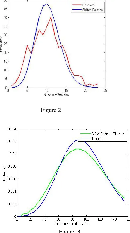
Figure 2 gives the observed frequency curve and expected frequency curve using shifted Poisson distribution for the number of fatalities. Figure 3 gives the plot for probability density functions of COM-Poisson Thomas and Thomas distributions.

Figure 2

244

7. CONCLUSION

In this paper, COM-Poisson Thomas distribution is defined and its properties are derived. Fatal accidents and fatalities data is analyzed and it is proved that COM-Poisson Thomas distribution is a better than Thomas distribution. The probability curves for COM-Poisson Thomas and Thomas distributions are plotted.

REFERENCES

[1] Conway R.W, and W.L. Maxwell. “A queuing model with state dependent service rates”, Journal of Industrial Engineering, 12, pp.132-136, 1962.

[2] Douglas J.B, “Analysis with Standard Contagious Distributions”, Burtonsville, MD: International Co-operative Publishing House. 1980.

[3] Feller W., “On a general class of “contagious” distribution”, Annals of Mathematical Statistics, 14, pp. 389-400, 1943.

[4] Johnson N.L, Kotz S and Kemp A.W “Univariate Discrete Distributions”, 3rd edition, Wiley Series in Probability and Mathematical Science, 2005.

[5] Neyman J. “ On a new class of “contagious” distributions, applicable in entomology and bacteriology”. The Annals of Mathematical Statistics 10, 1, pp. 35-57, 1939.

[6] Ord J.K “Families of Frequency Distributions”, London: Griffin, 1972.

[7] Shmeli G, Minka T.P, Kadane J.B, Borle S and Boatwright P, “A useful distribution for fitting discrete data: Revival of the COM-Poisson distribution”, J.R.Stat.Soc.Ser.C(Appl. Stat), 54, pp. 127-142, 2005.