Simulation and Comparison of Extended
Generalized Self Created Tree Explored Energy
Balance Routing Protocol for Wireless Sensor
Network
Raghavi G Kamat N. S. Sirdeshpande
PG Student Assistance Professor
Department of Electronics and Communication Engineering Department of Electronics and Communication Engineering Gogte Institute of Technology, Udyambhag, Belgaum-590008 Gogte Institute of Technology, Udyambhag, Belgaum-590008
Abstract
Wireless sensor network (WSN) is made up of a large number of less costly sensors. This network sends the receives the various kind of messages by using the base station. For WSN replacing the battery is not a easy task with large numbers of physically embedded nodes. There fore energy efficient routing protocol should be implemented to optimize the network life time of the wsn nodes. For this we need not only to balance WSN load but also to minimize total energy consumed. In this paper, we implement Extended Generalized Self-Created Tree Explored Energy-Balance routing protocol (EGSTEB) which builds a routing tree for each round, base station will select the root node and broadcasts this information to all its neighbor nodes. Simulation results show that EGSTEB is a dynamic protocol and has a good performance in balancing energy consumption by increasing the lifetime of WSN.
Keywords: Wireless Sensor Network, EGSTEB, Lifetime of Network, Sleep Mode, Self-Organized, WSN Load, Throughput of WSN Nodes
________________________________________________________________________________________________________
I.
INTRODUCTION
It is now possible to produce wireless sensor nodes in quantity at low cost with the advances in Micro-Electro-Mechanical Systems (MEMS)-based sensor technology, low-power digital electronics and low-power wireless communication.WSN collects large amounts of information and sends them to the Base Station (BS) with the help of large no of wireless sensor nodes. Usually Sensor nodes will get fused and deployed in the target area. After deployment, these nodes can not transfer data properly unless there is required battery is available. Many protocols use this data fusion technique and it assumes that the length of message transmitted will remain constant. In this paper, we are going to propose a Extended Generalized Self-Created Tree Explored Energy Balance routing protocol (EGSTEB).We define network lifetime in two different ways:(1) The time when the first node in the network dies(2) The time when the last node in the network dies.
Moreover, we consider two important cases in data fusion: Case (1) The data can be fused between any two sensor nodes. It first collects the data from its children’s and it send the data by adding its own amount of data. Case (2) The data can not be fused. The length of message received is the data of parent and also of its nearest neighbors data.
II.
LITERATURE SURVEY
The sensor nodes in the network will die quickly because of energy consumption if the BS is situated very far. On the other hand, direct transmission leads to unbalanced energy consumption, because the distances between each node and BS are different. Many protocols such as LEACH, PEGASIS and HEED are proposed to solve this problem.
For LEACH protocol the nodes first selects the cluster head for the fraction of the time t, where t is a design parameter. The LEACH operations are divided into several rounds. They include setup phase and a steady-state phase. In the first phase we will decide which node can be selected as cluster head. Each other nodes will join the cluster once the CH is selected. During the steady-state phase, using the single hop transmission the CH delivers the information to all its neighbor nodes. So this protocol can optimize WSN Load and reduce the amount of data transmitted to BS.
III.
EXTENDED GENERALIZED SELF-CREATED TREE EXPLORED ENERGY BALANCE ROUTIING PTOTOCOL
The operation of EGSTEB is divided into Initial set up Phase, Tree Constructing and path selection Phase, Self-Organized Data Collection and Transmission Phase, and Data Exchange Phase.
In first phase the BS selects the root node and broadcast this information to all other nodes. The sensor nodes which are very away from BS are put to sleep so the energy life time can be improved. In the second phase the network calculates the path either by transmitting the path selection information to sensor nodes to BS or by dynamically constructing the tree. For both cases mentioned above, EGSTEB can reconstruct the routing tree with low energy consumption and shorter delay because of less number of active nodes in the network. In third phase, each wireless sensor node generates a DATA_PKT which is then sent to BS. The information from each and every node is collected by using TDMA time slot. In fourth block, the data is transmitted to the base station. The EGSTEB protocol is compared with the other existing protocols like original GSTEB, LEACH. The simulation results showed that performance of EGSTEB is better than the others and it achieves the energy consumption.
IV.
METHODOLOGY
In our paper, we assume that the model has following important properties:
1) The wireless sensor nodes are distributed randomly in the square field and only one Bs is kept far away from target area. 2) Sensor nodes are not moving i.e they are stationary and energy effected. They will keep operating until their energy will
get over after the deployment.
3) Base station is stationary, but BS is not energy constrained. 4) Sensor nodes are location-aware.
5) Sensor nodes are put to sleep whenever they are not used by BS while selecting the neighbor nodes and also generating path from BS to neighbor nodes.
Initial Set up Phase: A.
In this phase node and network parameters are configured. This phase performs in three phases given below.
1) Step 1: When this Phase starts, BS broadcasts a starting time by sending the packet to all other nodes, the number of nodes N and length of time slot. After receiving the packet we will calculate their own energy-level equation(ELE) using function
ELE(k)=[residual Energy(k)/β]
ELE is a parameter for load balance, and it is an estimated energy. k is the ID of each node, and β is a dynamic the minimum energy value which can be changed based on our requirements.
2) Step 2: After the step 1 all nodes transmits the packet in the circle which has radius Rc in its own time slot. After all sensor nodes sends the data then it builds a table which has its own and neighbor node information.
3) Step 3: After the completion of step 2 ach node will be having its neighbors information. In the mean time we put the some nodes to sleep mode which are very far from BS. It means the node which are nearest to BS are only be
considered as active nodes. After Initial Phase, each node describes two tables in memory which has the information of all its neighbors and also of its neighbors neighbor.
Tree Constructing and Path Selection Phase: B.
For each round, ESTEB executes these three steps to build the routing tree . The steps to construct a routing tree for Case1 and Case2 are different:
1) Step 1: BS assigns a node as root node and broadcasts its selected root co-ordinates and root ID to all its neighbor sensor nodes. For Case1, a node with the greatest residual energy is selected as root node to balance the network load. In Case2 data can’t be fused, BS always first selects itself as root.
Self-Organized Data Collection and Transmission Phase: C.
After the generation of routing tree each sensor node constructs a DATA_PKT .We use TDMA technique for case 1.In a every time slot, only the leaf nodes can send their DATA_PKTs. After receiving all the data from its child nodes, It serves as a leaf node and sends the data fused in the next time slot. Each sensor node knows its parent ID. Every TDMA time slot has been divided into three segments as follow.
1) Segment1: In this segment, each leaf sensor node sends a packet which contains its root ID to its parent sensor node. The Three situations divide all the parent nodes into three category. For the first situation, the leaf node receives nothing. For the second situation, it receives a incorrect beacon, if more than one leaf sensor node needs to transmit information to the parent sensor node. For the third situation, it receives a correct beacon ,only if the leaf sensor node wants to transmit the data to its parent sensor node. The second segment operates on these three situations.
2) Segment 2: For the first situation, the parent node is put to sleep mode until the next time slot begins. For the second situation, the parent sensor node sends it control packet which has a control information to its child sensor nodes. This packet chooses one of its child node to send the information in next slot. For the third case, the parent sensor node transmits a control packet to this leaf node.
3) Segment 3: The parent sensor nodes receives the data from their leaf node, while other unused nodes put to sleep mode. For Case2, parent node is chosen by considering the total energy consumed by the node. In kth time slot, receives the message whose node ID is k. When all the data is received by BS , the network will begin the next phase.
Data Exchange Phase: D.
1) For Case1, since each node may die soon because it needs to generate and send a DATA_PKT . This process is also has three time slots. In every time slot, the sensor nodes loosing the energy, computes a random delay which allows only one sensor node to broadcast its information. While all other nodes performs the ID check after receiving the packet. The network will start the next round if it receives nothing.
2) For Case2, Base Station co-ordinates with other nodes by collecting the initial phase information and also EL value in the beginning . For each round, BS builds the schedule of the network and routing tree by using the coordinates information and EL. Once the routing tree is built, we can find the information needed to constructs a topography in next phase. The error flag is generated when actual EL is different from calculated EL of a sensor node are different, and this bundles residual energy of sensor node into DATA_PKT. After the receiving this DATA_PKT , BS will receives the original residual energy of this node and topology of next round is calculated by using this energy.
V.
RESULTS AND DISCUSSIONS
A NS2 simulation of EGSTEB protocol is done and it is compared with the original GSTEB protocol and also with the LEACH protocol. Table 1 defines the parameters we used to configure the nodes.
Table - 1
Parameters Used To Configure a Node Sl.No Parameter Name Parameter values
1 Channel type Wireless channel 2 Radio propagation model Two ray ground model
3 Mac type Mac 802_11
4 Antenna type Omni antenna
5 Number of nodes 42
6 Routing protocol AODV protocol
7 Time of simulation 60 ms
We are going to compare the original GSTEB protocol with the EGSTEB protocol for the following parameters. 1.Total Life Time 2.Throughput 3.End to End Delay
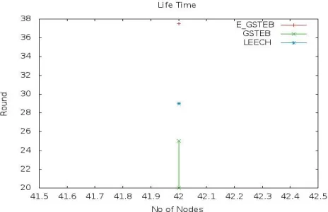
Fig. 1: Total Life Time comparison of EGSTEEB, GSTEB and LEACH Protocol.
Fig 1 describes the total life time of GSTEB with EGSTEB which is also compare with LEACH protocol. Which shows that the EGSTEB has life time of 37.5ms where as GSTEB has that of 25ms.Leach has very low life time compare to EGSTEB protocol. Fig 2 and fig 3 give the description about throughput and end to end delay of the wireless sensor network.
We observe from the fig 2 that the EGSTEB protocol has the throughput of 197bps and GSTEB has that of 171bps.The increase in the throughput of EGSTEB is because of the nodes which are put to sleeping mode when they are not reached by BS. Observing the fig 3 we can say that EGSTEB has a end to end delay of 41.10ms and GSTEB has that of 43.92ms.Which clearly proves that the EGSTEB transfers the packets fastly compared to GSTEB protocol.
Simulation results show that EGSTEB has higher total life time and throughput compare to GSTEB and LEACH protocol and also has less end to end delay.
REFERENCES
[1] WIKIPEDIA,"WIRELESS SENSOR NETWORKS , ”HTTP://EN.WIKIPEDIA.ORG/WIKI/WIRELESS_SENSOR_NETWORK
[2] K. AKKAYA AND M. YOUNIS, “A SURVEY OF ROUTING PROTOCOLS IN WIRELESS SENSOR NETWORKS,” ELSEVIER AD HOC NETWORK J., VOL. 3/3, PP. 325–349, 2005.
[3] I. F. AKYILDIZ ET AL., “WIRELESS SENSOR NETWORKS: A SURVEY,” COMPUTER NETW., VOL. 38, PP. 393–422, MAR. 2002.
[4] SOHRABI ET AL., “PROTOCOLS FOR SELF-ORGANIZATION OF A WIRELESS SENSOR NETWORK,” IEEE PERSONAL COMMUN., VOL. 7,
NO. 5, PP. 16–27,OCT. 2000.
[5] FRIEDEMANN MATTERN, KAY ROMER: “THE DESIGN SPACE OF WIRELESS SENSOR NETWORKS”, IEEE WIRELESS