Highly Complex Chaotic System with Piecewise
Linear Nonlinearity and Compound Structures
Wimol San-Um
Faculty of Engineering, Thai-Nichi Institute of Technology, Bangkok, Thailand Email: [email protected]
Banlue Srisuchinwong
Sirindhorn International Institute of Technology, Thammasat University, Pathum-Thani, Thailand Email: [email protected]
Abstract—A new chaotic system is presented using a single parameter for a two-scroll attractor with high complexity, high chaoticity and widely chaotic range. The system employs two quadratic nonlinearities and two piecewise-linear nonpiecewise-linearities. The high chaoticity is measured by the the maximum Lyapunov Exponent of 0.429 and the high complexity is measured by the Kaplan-Yorke dimension of 2.3004. Dynamic properties are described in terms of symmetry, a dissipative system, an existence of attractor, equilibria, Jacobian matrices, bifurcations, Poincaroé maps, chaotic waveforms, chaotic spectrum, and forming mechanisms of compound structures.
Index Terms— chaos, high-complexity, high-chaoticity, two-scroll attractor, piecewise-linear, compound structure
I. INTRODUCTION
The discovery of the eminent Lorenz system [1] has led to an extensive study of chaotic behaviors in nonlinear systems due to many possible applications in science and technology. The Lorenz system has seven terms in three-dimensional quadratic autonomous Ordinary Differential Equations (ODEs). Considerable research interests have also been made in exploring new chaotic systems either with simpler algebraic structures reflected by fewer terms in ODEs or with more chaotic and complex dynamical behaviors. A measure of chaoticity has been based on the Kaplan-Yorke dimension (DKY), whilst a measure of complexity (or strangeness) has been based on the maximum positive Lyapunov Exponent (LE).
Several chaotic systems have been suggested to retain two quadratic nonlinearities with fewer terms in ODEs and the attractors closely resemble the two-scroll Lorenz attractor. Examples of systems with six terms in ODEs include, Lu and Chen [2], Zhou et al.[3], Li et al., [4], Lui and Yang [5], Pehlivan and Glu [6], and Pan et al. [7] systems. Examples of systems with five terms in ODEs
include Sprott cases B and C [8], the diffusionless Lorenz system [9], and the five-term system [10]. Other systems have alternatively employed simpler piecewise-linear nonlinearities with five-terms in ODEs found in the jerk model [11], or a piecewise-linear Lorenz system [12]. Both systems are, however, lack of rotation symmetry [13]. Among all these systems, Sun and Sprott [14] have reported that the diffusionless Lorenz system has potentially possessed the highest value of DKY at 2.2354 through a single control system parameter. It can be considered that this diffusionless Lorenz system is simple in terms of algebraic structure with very high complexity in terms of DKY value.
Recently, two-scroll or many-scroll chaotic systems have employed more than two quadratic nonlinearities for generating complex chaotic attractors. For example, Li and Ou system [15] have employed three quadratic nonlinearities for a two-scroll complex attractor. Wang system [16] has employed three quadratic nonlinearities with eight-terms in ODEs for three-scroll and four-scroll attractors. Dadras et al. system [17] has realized four quadratic nonlinearities with eight-terms in ODEs for two-scroll, three-scroll and four-scroll attractors. Although many-scroll attractors have successfully been generated at the expense of extra three or four quadratic nonlinearities and a number of control parameters, the values of LE and DKY are only somewhat comparable to
those of chaotic systems with two quadratic
nonlinearities. In particular, the requirements for extra quadratic nonlinearities are not well suited to circuit implementations.
In this paper, a new chaotic system is presented using a single parameter for a two-scroll attractor with high complexity, high chaoticity and widely chaotic range. The system employs two quadratic nonlinearities and two piecewise-linear nonlinearities, including tanh and absolute value nonlinearity. Dynamic properties are theoretically and numerically described in terms of symmetry, a dissipative system, an existence of attractor, equilibria, Jacobian matrix, bifurcation diagram with period-doubling route to chaos, Poincaroé maps, chaotic waveforms in time domain, frequency spectrum, and forming mechanisms of compound structures.
II. PROPOSED HIGHLY COMPLEX CHAOTIC SYSTEM WITH
PIECEWISE-LINEAR NONLINEARITY
A new chaotic system is expressed as a set of three first-order autonomous differential equations with six-terms in ODEs as follows;
y xy R z (x) tanh z y x y x + + − = − = − = & &
& (1)
where x, y, z are system state variables and R is a single adjustable positive parameter. This new system (1) has been constructed through the realization of two quadratic and two piecewise-linear nonlinearities. The tanh and absolute value functions were found as potential nonlinearities that sustain two-scroll attractor topology similar to Lorenz attractor, but foster higher values of both DKY and LE.
III. SOME BASIC DYNAMICAL PROPERTIES
A. Symmetry, Dissipativity, and Existence of Attractor The system (1) is invariance under the coordinate transform (x,y,z)→(−x,−y,z), i.e. the system is symmetric around the z-axis and remains confined to the positive half-space with respect to the z state variable. The divergence of flow of the dynamic system is described as
. p z z y y x x
.V = =−1
∂ ∂ + ∂ ∂ + ∂ ∂ =
∇ & & & (2)
As p<0, the system systems (1) is a dissipative system with an exponential rate of contraction as
1). exp( exp(p)= −
= dt
dV (3)
In other words, a volume element V0 becomes smaller by the flow into a volume element V0exp(−t) in time t. Each volume containing the system trajectories shrinks to zero as t→∞ at an exponential rate of −1. System orbits are ultimately confined into a specific limit set of zero volume, and the system asymptotic motion settles onto an attractor. In conclusion, the existence of attractor is constant and independent to all of nonlinear terms. B. Equilibria
The equilibria of the system (1) can be found by using
0 0 tanh 0 = + + − = − = − y xy R (x) z x
y (4)
Consequently, the system possesses two equilibrium points, i.e. ). , R , R ( ) z , y , x ( P ), , R , R ( ) z , y , x ( P E E E E E E 0 2 4 1 2 1 2 4 1 2 1 0 2 4 1 2 1 2 4 1 2 1 + − − + − − = + + − + + − = − + (5)
It is seen from (5) that the single parameter R determines the existence of eqilibria. The two equilibrium points are almost symmetric, especially when R is large, and the
two-scroll attractor topology can be obtained. However, the equilibrium point at the origin as found in the Lorenz system does not exist in (5) and therefore the system (1) rather has a strong uniform flow in +z direction.
C. Jacobian Matrices and Stability
The Jacobian matrix (J) of partial derivatives of the system (1) is defined as
+ − − − = 0 0 0 1 1 2 ) x ( sign x y ) x tanh( z ) x ( tanh z
J . (6)
Applying the two equilibrium points described in (5) into this Jacobian matrix one at a time and analyzing |λI-J|=0
reveal a similar result of a characteristic polynomial, i.e.
0 2
2
3+ + + =
= / /
R R
J λ λ λ , (7)
where R/ in the case of the equilibrium point P+ is equal to
+ + − + + − = = + 2 4 1 2 1 2 4 1 2 1 R tanh R R
R/ / P
(8)
and R/ in the case of the equilibrium point P- is equal to
+ − − + − − = = − 2 4 1 2 1 2 4 1 2 1 R tanh R R
R/ / P
. (9)
Applying the Routh-Hurwitz criterion to (7) yields 0
2 =− <
− / /
/
R R
R . (10) It is verified from (10) that the parameter R must be positive for both equilibrium points in (5) so that the equilibrium points P+ and P- satisfy the unstable condition of Routh-Hurwitz criterion. In addition, the form of eigenvalues of the characteristic polynomial in (7) can only be one negative real eigenvalue λ1 and a pair of
complex conjugate eigenvalues λ
2 and λ3 with positive real parts. Therefore, the above analyses show that the two equilibrium points P+ and P- are all unstable, and can be classified as saddle focus nodes.
IV. NUMERICAL ANALYSIS
A.Bifurcations, Lyapunov Exponents, and Kaplan-Yorke Dimension
The Lyapunov exponents can be empoyed for the estimation of the rate of entropy production and the fractal dimension commonly known as
dimension DKY [18], i.e.
1 1
1 LE
k LE LE
j D
j
i i j
KY = +
∑
= += +
where k is a non-integer constant, and typically equals to 2 for three-dimensional chaotic system
summarizes chaotic regions for the parameter
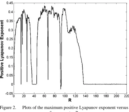
maximum LE (RLEmax), the LEs and the corresponding DKY. The system (1) has relatively wide chaotic range considered in five regions, including 0<
45<R<65, 67<R<92, and 93<R<134. Particularly, these five chaotic regions yield higher values of both maximum LE and fractional DKY compared with the diffusive Lorenz system that possesses the maximum
2.2354 at R=3.4693 where the LEs are (0.30791, 0, −1.30791). It is also seen from Table 1 that
positive LE of 0.4299 and the maximum occur in the region 45<R<65 where RLEmax can be chosen as a demonstrating numerical value
Figure 2. Plots of the maximum positive Lyapunov exponent versus the parameter R.
Figure 1. A bifurcation diagram exhibiting a period to chaos of the peak of z (‘z max’) versus the parameter
The Lyapunov exponents can be empoyed for the estimation of the rate of entropy production and the known as Kaplan-Yorke
3 2 1
LE LE
LE + . (11)
integer constant, and typically equals to dimensional chaotic systems. Table 1 the parameter R at the and the corresponding s relatively wide chaotic range five regions, including 0<R<14, 15<R<36, Particularly, these five chaotic regions yield higher values of both maximum compared with the diffusive the maximum DKY of s are (0.30791, 0, Table 1 that the maximum and the maximum DKY of 2.3004 LEmax is 60, which can be chosen as a demonstrating numerical value.
TABLE I. SUMMARY OF FIVE CHAOTIC REGIONS
VALUES OF RLE,MAX,
Regions RLEmax LE
0<R<14 R=12 (0.3696, 15<R<36 R=20 (0.4172, 45<R<65 R=60 (0.4299, 67<R<92 R=75 (0.4260, 93<R<134 R=98 (0.4210,
TABLE II.
SUMMARY OF EQUILIBRIUM POINTS AND THE COR EIGENVALUES OF JACOBIAN MATRICES AT
Equilibria Eigenvalues
P+(7.262,7.262, 0) λ1=-1.7124
λ 2,3=0.3562±2.8905
P-(-8.262,-8.262,0) λ1=-1.7333
λ 2,3=0.3667±3.0657
B.Numerical Equilibria and Eigenvalues
The system (1) can be formulated using the specific value of R at RLEmax= 60 as follows;
xy z
(x)z tanh y
x y x
+ − =
− =
− =
60
& & &
With reference to the previous analyses in ( Table 2 summarizes the numerical values of
points, the three eigenvalues of Jacobian matrices, and the corresponding types of equilibrium points at
60. As shown in Table 2, the attractor orbits around the two equilibrium points P+(7.262, 7.262, 0) and
-8.262,0), corresponding to the two
mostly symmetric shape. It is also evident that the two equilibrium points are saddle focus nodes as the eigenvalue λ1 is negative real value and
complex conjugate eigenvalues with positive real parts.
V. SIMULATION
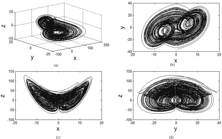
In the time domain, Fig. 3(a) shows apparently chaotic waveforms whilst an apparently continuous broadband spectrum log|x| in the frequency domain is shown in Fig. 3(b). It can be seen from Fig. 3 that the
chaotic behaviors. By using the Fourth Kutta method to solve the system (1
of 0.001, the chaotic attractors are displayed in Figs. 4(a)–(d) for a three-dimensional view, an
plane, an x–z phase plane and a
respectively. It is seen in Fig. 4(a) that the attractor of three-dimensional view remains confined to the positive half-space of the z-axis. In addition, the attractors apparently exhibit a two-scr
around the two equilibrium points and P-(-8.262, -8.262,0).
Figs. 5(a), (b) and (c) visualize the Poincaré maps in planes where x = 0, y = 0 and z
sheets of the attractors are displayed. It is noticeable that the Poincaré maps of many chaotic systems such as generalized Lorenz system [19] only show a
sitive Lyapunov exponent versus A bifurcation diagram exhibiting a period-doubling route
(‘z max’) versus the parameter R.
REGIONS, AND THE CORRESPONDING
LES, AND DKY.
LEs at p = -1 DKY
-0.0003 ,-1.3688) 2.2697 (0.4172,-0.0011,-1.4160) 2.2938 (0.4299,-0.0004,-1.4294) 2.3004 (0.4260, -0.0005,-1.4256) 2.2984 (0.4210,-0.0013,-1.4197) 2.2956
.
M POINTS AND THE CORRESPONDING ACOBIAN MATRICES AT RLEMAX=60.
Eigenvalues Equilibrium Points
Saddle Focus =0.3562±2.8905i
Saddle Focus =0.3667±3.0657i
Equilibria and Eigenvalues
The system (1) can be formulated using the specific = 60 as follows;
y xy (x)z
+
(12)
With reference to the previous analyses in (4) to (10), Table 2 summarizes the numerical values of equilibrium points, the three eigenvalues of Jacobian matrices, and the corresponding types of equilibrium points at RLEmax= As shown in Table 2, the attractor orbits around the (7.262, 7.262, 0) and P-(-8.262, 8.262,0), corresponding to the two-scroll attractor with mostly symmetric shape. It is also evident that the two equilibrium points are saddle focus nodes as the is negative real value and λ2,3 are a pair of
alues with positive real parts.
IMULATION RESULTS
In the time domain, Fig. 3(a) shows apparently chaotic whilst an apparently continuous broadband in the frequency domain is shown in Fig. an be seen from Fig. 3 that the system exhibits chaotic behaviors. By using the Fourth-order Runge-Kutta method to solve the system (12) with time step size of 0.001, the chaotic attractors are displayed in Figs. dimensional view, an x–y phase phase plane and a y–z phase plane, respectively. It is seen in Fig. 4(a) that the attractor of dimensional view remains confined to the positive axis. In addition, the attractors scroll topology that orbits around the two equilibrium points P+(7.262, 7.262, 0)
with several twigs. The Poincaré maps in Figs. 5(a) and (b), however, consist of virtually symmetrical branches and a number of nearly symmetrical win
is clear that some sheets are folded.
VI. FORMING MECHANISMS OF COMPOUND
Compound structures [20] generally demonstrate a forming mechanism of attractor, clarifying its topological structure. The compound structures of the system (12) may be demonstrated using a half-image operation to obtain only the left or the right half-image attractors, both of which can then be merged together as a compound structure. Such an operation can be revealed through the use of a controlled system of the following form
(c) (d)
Figure 4. Chaotic attractors, (a) a three
(a)
Figure 3. (a) apparently chaotic waveform
(a)
with several twigs. The Poincaré maps in Figs. 5(a) and (b), however, consist of virtually symmetrical branches ngs. In Fig. 5(c), it
OMPOUND STRUCTURES
Compound structures [20] generally demonstrate a forming mechanism of attractor, clarifying its topological ompound structures of the system (12) image operation to image attractors, both of which can then be merged together as a compound structure. Such an operation can be revealed through the
following form
xy z
(x)z y
x y x
+ − =
− =
− =
60 tanh
& & &
where u is a control parameter.
image of the original attractor shown in Fig. isolated as illustrated in Fig. 6(a) for the In contrast, when u = 15, another right half
original attractor can be isolated as illustrated in Fig. 6(b) for the y–z phase plane. It is evident
and right-image of the attractor in
(13) consists of compound structures, which ultimately form the two–scroll attractor topology as previously depicted in Fig.4 (d).
(c) (d)
three-dimensional view, (b) an x–y phase plane, (c) an x–z phase plane, (d) (b)
pparently chaotic waveforms, (b) an apparently continuous broadband frequency spectrum log
x(t) y(t) z(t)
(b)
y xy
u (x)z
+
+ (13)
is a control parameter. When u = −15, a left half-image of the original attractor shown in Fig. 4(d) can be isolated as illustrated in Fig. 6(a) for the y–z phase plane. = 15, another right half-image of the original attractor can be isolated as illustrated in Fig. 6(b) plane. It is evident in both left-image image of the attractor in Fig. 6 that the system consists of compound structures, which ultimately scroll attractor topology as previously
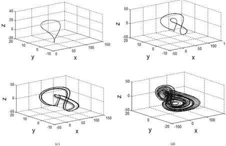
Fig. 7 demonstrates gradual development of forming mechanisms of such compound structures. Different dynamical behaviors can be summarized as follows; (a) When |u| ≥ 36, the system (13) has limit cycles. For
example, Fig. 7(a) shows a limit cycle at u = 40. (b) When 23≤ |u| ≤ 36, the system (13) also has limit
cycles, forming different characteristics. For example, Fig. 7(b) shows a limit cycle at u = 30. (c) When 6≤ |u| ≤ 23, the system (13) demonstrates
period-doubling bifurcations. For example, Fig. 7(c) shows such period-doubling bifurcations at u = 14. (d) When |u| ≤ 6, the system (13) exhibits a partially
complete attractor as shown in Fig. 7(d) at u = 5. VII.COMPARISONS OF CHAOTICITY AND COMPLEXITY
Table 3 summarizes the chaoticity and complexity between this paper and related references. For chaoticity, the divergence of flow p typically affects the values of LEs and consequently sets the chaoticity measured by the positive LEmax. It is evident from Table 1 that this paper possesses the highest LEmax of 0.4299 compared to the systems [9] and [12] in which p is optimally simple at -1. Although the smaller values of p in systems [1], [10], [12], [17] and [21] results in a higher values of LEmax, the negative LE is also decreased correspondingly, retaining the constant DKY as described in (11).
For complexity, this paper has offered the highest value of DKY=2.3004. It is seen from Table 3 that the use of only piecewise-linear nonlinearity in [12] offers a
TABLE III.
CHAOTICITY AND COMPLEXITY OF THE SYSTEM (1) DEVELOPED IN THIS PAPER COMPARED TO THOSE OF OTHERS.
Ref. Chaoticity Complexity
p LEs DKY
[1] -13.67 (0.90564, 0, −14.572 31) 2.0621 [9] -1 (0.30791, 0, −1.307 91) 2.2354 [10] -5 (1.4913, 0.0026,-6.4939.) 2.2301 [12] -1 (0.0652, 0, −1.0652) 2.0612 [15] -12 (0.426531, 0, −7.426415) 2.0574 [17] -10.9 (0.559156, 0, -11.444555) 2.0488 [21] -11 (2.6148, 0, -13.6148) 2.1921 This paper -1 (0.4299,-0.0004,-1.4294) 2.3004
relatively low DKY while the use of two nonlinearity in [9], [10], and [20] offer higher DKY. In addition, the systems [15] and [17] require at least three quadratic nonlinearities with higher number of terms in ODEs, but the DKY is relatively low. The proposed chaotic system has attempted for more complex attractors through the interaction of two quadratic and two piecewise-linear nonlinearities, resulting in higher values of both chaoticity and complexity. Furthermore, circuit implementations for tanh and absolute value functions are relative simple based on a single saturated amplifier and a signum nonlinearity circuit [18]. Therefore, the proposed system offers a potential alternative to highly complex chaotic system, but the possible implementation is simple.
(c)
Figure 5. Poincaré maps in planes where (a) x = 0, (b) y = 0, (c) z = 0.
CONCLUSIONS
The new chaotic system has been presented single parameter and a two-scroll attractor. The system has employed two quadratic nonlinearities and two piecewise-linear nonlinearities with only six
ODEs. The system achieved high chaoticity of high complexity of 2.3004. Dynamic properties been described in terms of symmetry,
system, an existence of attractor, equilibria, Jacobia matrix, bifurcations, Poincaré maps, waveforms, spectrum, and forming mechanisms of compound structures. This work offers a potential alternative to chaotic systems in applications of chaos to control and communication systems.
(c) (d)
Figure 7. Phase portraits of the system (13) at (a)
(b)
Figure 6. (a) a left half-image attractor for the y
system has been presented with a scroll attractor. The system nonlinearities and two linear nonlinearities with only six-terms in high chaoticity of 0.429 and 2.3004. Dynamic properties have symmetry, a dissipative of attractor, equilibria, Jacobian
é maps, waveforms,
spectrum, and forming mechanisms of compound a potential alternative to in applications of chaos to control and
REFERENCES
[1] E.N. Lorenz, “Deterministic Atmosphere and Science, vol. 20,
[2] J. Lü, G. Chen. “A New Chaotic Attractor Coined.” Bifurcation and Chaos, vol. 12
[3] W. Zhou, Y. Xu, H. Lu, and L. Analysis of a New Chaotic Attractor”, vol. 372, 2008, pp. 5773-5777
[4] X. F. Li, Y. D. Chu, J. G. Zhang, Y.X. Chang, “ Dynamics and Circuit Implementation for a New Lorenz like Attractor”, J. Chaos, Solitons &
5, 2009, pp. 2360-2370.
[5] Y. Liu, Q.Yanga, “Dynamics of a New Lorenz Chaotic System”, J. Nonlinear Analysis: Real World Applications, vol. 11, 2010, pp. 2563
[6] Í. Pehlívan, Y. Uyaroĝlu, “A New Chaotic Attractor From General Lorenz System Family and iIts Electronic
(c) (d)
Phase portraits of the system (13) at (a) u= 40, (a) u= 30, (a) u= 14, (a) u= 5. (b)
image attractor for the y-z plane at u= -15, (b) a right half-image attractor for the y
EFERENCES
Deterministic Nonperiodic Flow” J. ol. 20, 1963, pp. 130.
J. Lü, G. Chen. “A New Chaotic Attractor Coined.” J. 12, No. 3, pp. 659-661, 2002. Y. Xu, H. Lu, and L. Pan, “On Dynamics
Attractor”, J. Physics Letter A, 5777.
X. F. Li, Y. D. Chu, J. G. Zhang, Y.X. Chang, “Nonlinear Dynamics and Circuit Implementation for a New
Lorenz-Chaos, Solitons & Fractals, vol. 41, No.
Dynamics of a New Lorenz-like J. Nonlinear Analysis: Real World
, pp. 2563-2572.
A New Chaotic Attractor From General Lorenz System Family and iIts Electronic
Experimental Implementation”, Turk J. Electrical Engineering & Computer Science, vol.18, No.2, 2010, pp.171-184.
[7] L. Pan, D. Xu, W. Zhou, “Controlling a Novel Chaotic Attractor using Linear Feedback”, J. Information and Computing Science, vol. 5, No. 2, 2010, pp.117-124. [8] J. C. Sprott, “Some Simple Chaotic Flows”, J. Physical
Reviews E, Vol. 50, 1994, pp.647-650.
[9] G. Schrier , L.R.M. Maas, “The Diffusionless Lorenz Equations; Shil’nikov Bifurcations and Reduction to an Explicit Map, J. Physiscs D, vol. 141, 2000, pp. 19-36. [10]B. Munmuangsaen, B. Srisuchinwong, “A New Five-Term
Simple Chaotic Attractor”, J. Physics Letters A, vol. 373, No. 44, 2009, pp. 4038-4043.
[11]J. C. Sprott, “Simplifications of the Lorenz Attractor”, J. Nonlinear Dynamics, Psychology, and Life Sciences, vol. 13, No. 3, 2009, pp. 271-278.
[12]A. S. Elwakil, S. Özôguz, M. P. Kennedy,” Creation of a Complex Butterfly Attractor Using a NovelLorenz-Type System”, IEEE Transaction on circuits and systems I, vol. 49, No. 4, 2002, pp.527-530.
[13]33J.-M. Malasoma, “What is the Simplest Dissipative Chaotic Jerk Equation Which is Parity iInvariant”, J. Physics Letters A, Vol. 264, 2000, pp. 383–389.
[14]J. C. Sprott, “Maximally Complex Simple Attractors”, Int. J. Chaos, vol. 17, 2007, pp. 033124.
[15]X. Li, Q. Ou,” Dynamical Properties and Simulation of a New Lorenz-like Chaotic System”, J. Nonlinear dynamics, doi:10.1007/s11071-010-9887-z.
[16]L. Wang,” 3-Scroll and 4-Scroll Chaotic Attractors Generated from a New 3-D Quadratic Autonomous System” J. Nonlinear dynamics, vol. 56, 2009, pp. 453– 462.
[17]S. Dadras, H. R. Momeni, G. Qi, “Analysis of a New 3D Smooth Autonomous System with Different Wing Chaotic Attractors and Transient Chaos”, J. Nonlinear dynamics, Vol. 62, pp. 391–405, 2010.
[18]J.C. Sprott, "Elegant Chaos: Algebraically Simple Chaotic Flows", World Scientific Publishing Company, 2010. [19]S. Celikovsky, C.Guanrong, “On the Generalized Lorenz
Canonical Form”, J. Chaos Solitons and Fractals, vol. 5, 2005, pp.1271-1276.
[20]J. Lu, G. Chen, S. Zhang, “The Compound Structure of a new Chaotic Attractor”, J. Chaos, Solitons and Fractals, Vol. 14, 2002, pp. 669-672.
[21]B. Srisuchinwong, B. Munmuangsaen, “A Highly Chaotic Attractor for a Dual-Channel Single-Attractor, Private Communication System”, Proceedings of the 3rd Chaotic Modeling & Simulation International Conference, 2010, pp. 177(1-8).
Wimol San-Um was born in Nan Province, Thailand in 1981. He received BEng Degree in Electrical Engineering and MSc Degree in Telecommunications in 2003 and 2006, respectively, from Sirindhorn International Institute of Technology, Thammasat University, Thailand. In 2007, he was a research student at University of Applied Science Ravensburg-Weingarten, Germany. He received PhD in LSI Designs in 2010 from the Department of Electronic and Photonic System Engineering, Kochi University of Technology, Japan. He is a lecturer at Computer Engineering Program, Faculty of Engineering, Thai-Nichi Institute of Technology. His areas of research interests are analog integrated circuit designs, involving chaotic oscillators and switched-current circuits, and on-chip testing design, involving DFT and BIST techniques.
Banlue Srisuchinwong was born in Bangkok, Thailand in 1963. He received the BEng (Hons) degree in Electrical Engineering from King Mongkut's Institute of Technology Ladkrabang, Thailand, in 1985, the Diploma of the Philips International Institute of Technological Studies (electronics), the Netherlands, in 1987, the MSc and the PhD degrees from University of Manchester Institute of Science and Technology (UMIST), UK, in 1990 and 1992, respectively. Since 1993, he has been with Sirindhorn International Institute of Technology (SIIT), Thammasat University, Thailand, where he is currently an Associate Professor of Electrical Engineering.