www.earth-surf-dynam.net/5/21/2017/ doi:10.5194/esurf-5-21-2017
© Author(s) 2017. CC Attribution 3.0 License.
Creative computing with Landlab: an open-source toolkit
for building, coupling, and exploring two-dimensional
numerical models of Earth-surface dynamics
Daniel E. J. Hobley1,2,3, Jordan M. Adams4, Sai Siddhartha Nudurupati5, Eric W. H. Hutton6, Nicole M. Gasparini4, Erkan Istanbulluoglu5, and Gregory E. Tucker1,2
1Cooperative Institute for Research in Environmental Sciences (CIRES), University of Colorado, Boulder, USA 2Department of Geological Sciences, University of Colorado, Boulder, USA
3School of Earth and Ocean Sciences, Cardiff University, Cardiff, UK
4Department of Earth and Environmental Sciences, Tulane University, New Orleans, USA 5Department of Civil and Environmental Engineering, University of Washington, Seattle, USA
6Community Surface Dynamics Modeling System (CSDMS), University of Colorado, Boulder, USA
Correspondence to:Daniel E. J. Hobley ([email protected])
Received: 20 August 2016 – Published in Earth Surf. Dynam. Discuss.: 14 September 2016 Revised: 24 November 2016 – Accepted: 14 December 2016 – Published: 16 January 2017
Abstract. The ability to model surface processes and to couple them to both subsurface and atmospheric regimes has proven invaluable to research in the Earth and planetary sciences. However, creating a new model typically demands a very large investment of time, and modifying an existing model to address a new prob-lem typically means the new work is constrained to its detriment by model adaptations for a different probprob-lem. Landlab is an open-source software framework explicitly designed to accelerate the development of new process models by providing (1) a set of tools and existing grid structures – including both regular and irregular grids – to make it faster and easier to develop new process components, or numerical implementations of physical pro-cesses; (2) a suite of stable, modular, and interoperable process components that can be combined to create an integrated model; and (3) a set of tools for data input, output, manipulation, and visualization. A set of example models built with these components is also provided. Landlab’s structure makes it ideal not only for fully devel-oped modelling applications but also for model prototyping and classroom use. Because of its modular nature, it can also act as a platform for model intercomparison and epistemic uncertainty and sensitivity analyses. Landlab exposes a standardized model interoperability interface, and is able to couple to third-party models and software. Landlab also offers tools to allow the creation of cellular automata, and allows native coupling of such models to more traditional continuous differential equation-based modules. We illustrate the principles of component coupling in Landlab using a model of landform evolution, a cellular ecohydrologic model, and a flood-wave routing model.
1 Introduction and motivation
Across a wide array of fields, researchers use numerical mod-els to study processes that operate on and across the Earth’s land surface and shallow subsurface. Science and engineer-ing applications of these models of surface dynamics range from short-term flood forecasting (e.g. Horritt and Bates, 2002) to simulating the evolution of Earth’s landscape over
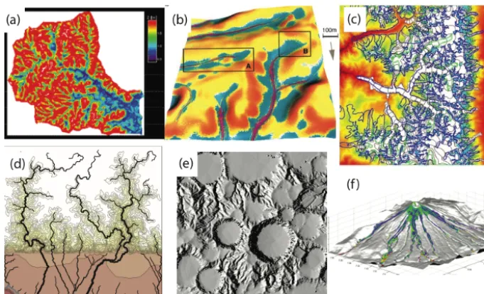
algo-Figure 1.Examples of surface-process models.(a)Computed depth-to-groundwater, from the GSEM coupled groundwater–surface water model (Berger, 2000, image courtesy D. Entekhabi).(b)Computed patterns of soil erosion and sedimentation on agricultural fields, using the SIMWE soil erosion model (Mitas and Mitasova, 1998). (c)Model of ice-age glacier extent over the Sierra Nevada, USA, using the GC2D ice-flow model (Kessler et al., 2006).(d)Simulation of canyon erosion and fan-delta progradation in a region of active uplift (top) and subsidence (bottom), using the CHILD landscape evolution model (Tucker and Hancock, 2010).(e)Model of simultaneous cratering and fluvial erosion on the ancient Mars surface, with the MARSSIM model (Howard, 2007).(f)Simulation of pyroclastic flows at Tungurahua volcano, Ecuador, using the VolcFlow model (Kelfoun et al., 2009).
rithms to represent a terrain surface and its connectivity, and many include solution algorithms to compute flows of mass (such as ice, liquid water, sediment, or chemical nutrients) across terrain (Slingerland and Kump, 2011) (Fig. 1).
However, scientists who want to use an Earth-surface model often build their own unique model from the ground up, re-coding the basic building blocks of their model rather than taking advantage of codes that have already been writ-ten (Adams et al., 2014; Katz et al., 2015; Overeem et al., 2013). This undoubtedly does produce novel software capa-ble of fulfilling its designer’s needs, and can have advantages in helping the programmer to acquire a total understanding of the code base, but this approach also has many associ-ated problems: many person hours are lost rewriting exist-ing code, and the resultexist-ing software is often idiosyncratic, ad hoc, undocumented, and unable to interact with other soft-ware programs both in the same scientific community and beyond. In particular, models are often initially written to solve a very specific problem, rather than to provide a flexible and reliable platform for solving a general class of problems (Easterbrook, 2014). It may also become impossible for a single programmer to maintain their grasp of their code base once it exceeds a certain size. A result is that software devel-opment often acts as a bottleneck to progress, with frequent duplication of effort as research groups struggle to adapt ex-isting software or develop new code from the ground up as each new research problem emerges.
The Landlab modelling framework described here seeks to mitigate these redundancies and lost opportunities and simul-taneously lower the bar for entry into numerical modelling. The approach is to create a user- and developer-friendly mod-elling environment that provides scientists with the funda-mental building blocks needed for modelling surface dynam-ics on the Earth, and potentially beyond. The framework takes advantage of the fact that nearly all surface-dynamics models share a set of common software elements, despite the wide range of processes and scales that they encompass (Peckham et al., 2013; Slingerland and Kump, 2011). Pro-viding these elements in the context of the popular scientific programming language Python, and with strong user support and community engagement, would contribute to accelerat-ing progress in the diverse sciences of the Earth’s surface.
From the user’s perspective, Landlab enables the follow-ing:
1. Rapid, easy creation of a number of distinct geomet-ricgrids, with all the connectivity between various el-ements already defined, and the ability to create two-dimensional data fields across a given grid.
2. Functions to operate on the values defined on such a grid, enabling the solution of time-dependent numeri-cal algorithms across them (e.g. differential equations, cellular automata).
4. Encapsulation of conceptual models for individual Earth-surface processes into reusablecomponents, with a standard interface that allows operation across Land-lab grids.
5. The ability to build a multi-process model by combining together components.
6. The ability to quickly and efficiently build new com-ponents, and to couple them with those components al-ready in the library.
7. A straightforward and standardized input and output in-terface, including the ability to import from and export to common spatially distributed data formats such as NetCDF and ESRI ASCII, as well as a plotting mod-ule. This interface also enables coupling to third-party models and software.
2 Approach
2.1 Guiding design principles
The design principles for Landlab have been guided both by our observations of current software design practices in the surface-system modelling community and by white papers issued by existing organizations both within this community (Adams et al., 2014; Overeem et al., 2013; Peckham et al., 2013) and in the scientific software design community more widely (Becker et al., 2015; Chue Hong, 2014; Katz et al., 2015; NSF, 2012). Our key observations are as follows:
1. Many models exist that simulate Earth-surface pro-cesses, and many of these share a very similar under-pinning in terms of the basics of grid construction and the suite of simulated processes. This set of models rep-resents significant past duplicative effort in the surface process modelling community. Although the reasons for duplication are likely multiple and vary from group to group, we note that we are unaware of previous ef-forts to advertise a flexible, open-source programming framework.
2. Orphaned or unmaintained codes are common in the re-search community, having been built for a single pur-pose and then set aside.
3. Although standardized frameworks for model interop-erability are now in place (such as the framework de-signed and maintained by the Community Surface Dy-namics Modelling System, CSDMS, group; Hutton et al., 2014; Overeem et al., 2013; Peckham et al., 2013), many models are not compatible with these standards. We hypothesize this is largely due to the effort required by the original programmer to modify legacy code – which in many cases was written before the standards were established – to meet these new interoperability criteria.
4. Existing model software tends to have a high bar to en-try. Many models are written in compiled languages, such as Fortran, C, and C++ (examples from the ge-omorphology and sedimentary stratigraphy communi-ties include CHILD: Tucker et al., 2001b; Sedflux: Hut-ton and Syvitski, 2008; MARSSIM: Howard, 2007; Fastscape: Braun and Willett, 2013; DAC: Goren et al., 2014; SIBERIA: Willgoose et al., 1991a, b). This re-quires the prospective user be fluent in these languages before the code can be modified or, in many cases, even used efficiently. Because many legacy codes were not designed to be shared amongst the community, docu-mentation, both in-line and external, tends to be idiosyn-cratic at best and missing at worst.
5. In several instances, scientific software with a broad user base exists but remains closed source. This includes both tools for data analysis (e.g. ArcMap, Matlab) and in some cases the modelling software itself (e.g. FLAC; Itasca, 2000; Dionisos, Granjeon and Joseph, 1999). Where software has to be purchased, this presents ob-vious barriers to wide uptake of modelling approaches using these tools in terms of financial cost for the user. More importantly, all closed-source software also presents significant barriers to code assessment in peer review and to reproducibility of the work (Crick et al., 2014; Katz et al., 2015).
These observations lead us to a set of key design principles that have governed our development of Landlab:
a. Landlab should be a community resource, and thus fully
open source.
b. Landlab should provide a development environment that isflexible, extensible, and highly reusable. c. Landlab should be written in a language that allows
rapid developmentof new code.
d. Landlab should be fully compliant with the CSDMS model interoperability standards (Peckham et al., 2013) from the ground up, and this compliance should be built into the low-level development framework itself. Thus, for example, components written in Landlab will be au-tomatically compliant with these standards.
e. Landlab should have alow bar to entryand be thor-oughly documented. Tutorials should be present. It should be possible for a beginner to use Landlab with-out a full grasp of the underlying model architecture, in a “plug and play” fashion.
2.2 Low-level design choices
In turn, these guiding design principles directed early deci-sions in terms of Landlab’s coding language, architecture, and distribution.
2.2.1 Open-source availability
Landlab is licensed under the MIT free software license, an approved license of the Open Source Initiative. This license allows a user to deal in the software without restriction, in-cluding without limitation the rights to use, copy, modify, merge, publish, distribute, sublicense, and/or sell copies of the software. The source code and associated files are main-tained in a Git version-control repository, for which the mas-ter repository is presently hosted on the GitHub website, https://github.com/landlab/landlab. Release versions are also freely available through thepipandcondaPython package managers. The model repository maintained by CSDMS of-fers links to Landlab documentation and to the GitHub repos-itory, increasing Landlab’s visibility to the surface process modelling community in particular. Web-based documenta-tion is hosted at http://landlab.github.io. This includes both developer-written summary documents and tutorials, as well as reference-level documentation that is automatically gener-ated from inline comments and examples in the code itself.
2.2.2 Programming language
Landlab is written in Python and exploits and includes as de-pendencies a number of widely used scientific Python pack-ages: numpy, scipy, matplotlib, nose, netCDF4, numpydoc, cython, six, pyyaml, setuptools, and libgcc. The decision to write in Python was explicitly made to lower the bar for entry to Landlab, to increase the flexibility and reusability of the code base, and to increase development speed both for the core development team and for future users. Informal can-vassing amongst the surface process community, especially amongst graduate students and other early-career scientists less likely to already be strongly wedded to a certain de-velopment environment, revealed a marked preference for – and greater familiarity with – Python over C+ +(other open-source languages were rarely mentioned). This chang-ing preference for Python has also been noted for PhD stu-dents in general, beyond just the field of surface process mod-elling (Chue Hong, 2014). The choice of Python also means that developers using Landlab can take advantage of that lan-guage’s affinity for rapid development (Prechelt, 2000). In particular, Python’s dynamic typing and interpreted rather than compiled implementation remove the developer’s need to deal explicitly with memory management (van Rossum and Drake, 2001). Other advantages of this choice include high portability between platforms, open-source language, numerous existing scientific libraries, and support for selec-tive optimization of time-critical parts of the code base us-ing Cython and/or compiled-language extensions. Cython is
a compiled language that is a super-set of Python, and Cython extension modules interact seamlessly with pure Python. However, program modules written in Cython allow more granular control of memory management than is the case in pure Python, which can result in significant acceleration of code. Cython is already in use within Landlab for sections of the code that require long out-of-sequence iterations through arrays, and other sections where pure Python would tend to have poor performance. For example, Cython is used in the construction of some of the grid element connectivity arrays, in the FlowRouter and FastscapeEroder components, and in the CellLab extension to Landlab (Tucker et al., 2016).
2.2.3 Code sustainability
A key objective for Landlab from inception has been that the code base be sustainable (Adams et al., 2014; Becker et al., 2015; Katz et al., 2015; Stewart et al., 2010). Following other authors, we view sustainable software as that which is able to continue effectively, sustaining or improving its functionality through time while at the same time adding new users. Stew-art et al. (2010) drew attention to a number of key features of sustainable software, which we have sought to implement:
– Strong, consistent leadership.The authors of this paper represent the core development team of Landlab.
– Rapid prototyping and evolutionary design. Landlab was initially developed to fill the immediate research needs of the core development team, giving it a strong and well-defined initial direction. In this initial develop-ment phase, we have emphasized long-term mountain belt evolution modelling; steady- and nonsteady-flow routing; eco-, surface, and shallow subsurface hydrol-ogy; hillslope dynamics; cellular automaton modelling; vegetation dynamics; and ecosystem dynamics. How-ever, the explicitly modular nature of Landlab means that it can readily adapt to new scientific objectives and expand to meet new and as yet unforeseen demands in the future.
tutorials are created and maintained manually. Auto-generated documentation is updated and posted to the project website automatically as new code changes are committed to the GitHub repository using “webhook” functionality provided through the http://readthedocs. org website.
– Sustained compatibility with underlying libraries, pro-tocols ,and operating systems. Landlab is compatible both with Python 2 and 3. The code base is tested au-tomatically using Travis (Mac, Unix) and Appveyor (PC) continuous integration platforms, across Python versions 2.7, 3.4, and 3.5 (see also Sect. 4).
– Dissemination and community understanding. We have sought to publicize Landlab widely at a number of international conferences and workshops, classes, and through collaborative networks. We estimate that, as of mid-2016, approximately 330 potential users have now seen or participated in Landlab-based presentations or classes.
– Encouraging collaborative software development. Landlab enables users to tailor its functionality to their specific needs, through its modular design and flexible grid and grid functions. We are already aware of a num-ber of groups outside the core Landlab development team working with Landlab for their own research purposes.
A secondary aspect to sustainability is the ability to have the software continue to be useable after the active devel-opment cycle has ceased (Stewart et al., 2010). We antici-pate that the choice of Python, minimal system and extension package requirements, open-source availability of our code base, and thorough documentation will sustain our code for the foreseeable future.
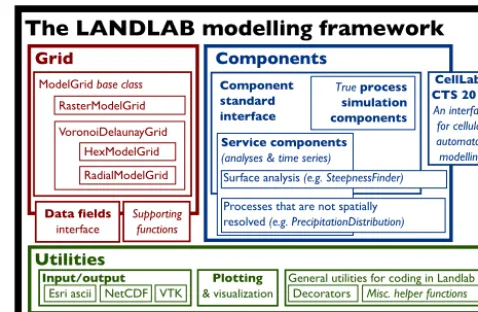
3 Model architecture
Landlab has an essentially tripartite structure – a core grid module, a library of process components, and a set of sup-porting utilities (Fig. 2). The various subdivisions of the code behave as Python modules and can be imported and used within a Python environment independently.
3.1 Landlab’s gridding engine
Landlab provides the ability to create a two-dimensional sim-ulation grid of a user-specified size and shape, with a sin-gle line of code. Grids are represented as Python objects; a grid object includes data describing its geometry and topol-ogy, as well as a variety of methods and functions to manage data and perform common numerical operations. (In object-oriented programming parlance, amethodis a procedure as-sociated with an object; in this case, “method” means a
func-Grid
RasterModelGrid
VoronoiDelaunayGrid HexModelGrid RadialModelGrid
Data fields
interface
Supporting functions
Components
Component standard interface
True process simulation components Service components
(analyses & time series)
Surface analysis (e.g. SteepnessFinder)
Processes that are not spatially resolved (e.g. PrecipitationDistribution)
ModelGrid base class
Utilities
Plotting & visualization Input/output
Esri ascii NetCDF VTK
CellLab-CTS 2015
An interface for cellular automaton modelling
General utilities for coding in Landlab Decorators Misc. helper functions
The LANDLAB modelling framework
Figure 2.Schematic illustration of the structure of Landlab 1.0. The three main divisions of the code are the grid, the components, and supporting utilities. Structure within these three main divisions is discussed in the main text.
tion that is defined within the grid class, and that can be ac-cessed with the “grid.method()” syntax typical of other class properties.)
Although Landlab grids are inherently two-dimensional, in many cases it is nonetheless possible to create an effec-tively one-dimensional simulation by creating a 3-by-N regu-lar grid and closing the nodes along the top and bottom edges (see Sect. 3.1.4). Three-dimensional grids are not possible in Landlab at this time, though they may be supported in a fu-ture release.
3.1.1 Grid types and elements
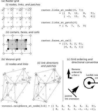
A Landlab grid is defined by a set of grid primitive elements: nodes, links, cells, corners, faces, and patches (Fig. 3). In terms of graph theory, these can be thought of as two inter-locking and offset sets of points (nodes vs. corners), edges (links vs. faces), and areas (patches vs. cells). The entire grid can be generated from a description of the geometry of only one of these element types – typically, a user might spec-ify the locations of the nodes, and the grid object’s remain-ing elements are automatically placed accordremain-ing to this node framework.
(a) Raster grid (b) Voronoi cells with Delaunay triangulated nodes
Cell Patch Node Corner Face Link
(c) Hexagonal grid
Figure 3.Geometry and topology of grid elements on various Landlab grids. Only one patch and its bounding links are shown for each example to prevent the diagram from becoming cluttered. Links always point into the upper right semicircle, as described in the text.
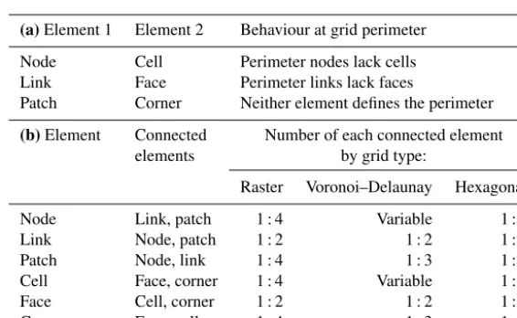
Table 1.(a)One-to-one mappings of Landlab grid elements.(b)Primary one-to-many mappings of Landlab grid elements.
(a)Element 1 Element 2 Behaviour at grid perimeter
Node Cell Perimeter nodes lack cells
Link Face Perimeter links lack faces
Patch Corner Neither element defines the perimeter
(b)Element Connected Number of each connected element
elements by grid type:
Raster Voronoi–Delaunay Hexagonal
Node Link, patch 1 : 4 Variable 1 : 6
Link Node, patch 1 : 2 1 : 2 1 : 2
Patch Node, link 1 : 4 1 : 3 1 : 3
Cell Face, corner 1 : 4 Variable 1 : 6
Face Cell, corner 1 : 2 1 : 2 1 : 2
Corner Face, cell 1 : 4 1 : 3 1 : 3
one-to-one mappings of features, and emphasizes which el-ement defines the grid edge in each case. Table 1b lists the primary one-to-many relationships defined for each element type, and lists the standard number of mapped elements (if well defined) for each of the primary grid classes. Note that this table only lists the most useful identities within the three-element groupings node-link-patch and cell-face-corner. The other identities also exist and can be reconstructed from the one-to-one identities in Table 1a.
Data can be assigned to any element of the grid (see Sect. 3.2, below). The grid classes also provide prop-erties that define and describe the geometric interrela-tionships amongst these grid elements (see, e.g., Fig. 4). These mappings allow common geometric operations (such as calculation of gradients across the grid, finding max-imum/minimum/mean values of neighbours, upwinding schemes, and flux divergences) to be achieved in typically one or two lines of code.
Landlab provides native support for both regular and irreg-ular grids (Figs. 3, 4). Treating both grid types natively within Landlab allows the grid to be tailored to specific applications. For example, raster grids provide compatibility with digital elevation model data, and can in some cases allow better
op-timized process algorithms. Trigonal grids with hexagonal cells provide an additional axis of symmetry, and obviate the need for handling diagonal connections in certain types of numerical algorithm (such as flow routing; e.g. Jenson and Domingue, 1988). Irregular grids avoid some of the cardi-nal direction artifacts than can form on regular grids, such as linear networks and linear drainage divides, as well as conse-quent biases in measured channel metrics like drainage den-sity, river length, and channel slope (Braun and Sambridge, 1997).
frame-(a) Raster grid
0 1
2 3
4 5
6 7
8
9
0 0
1 2
3 4
5 8
6 7 16
9 10
13 12 14 11
15 17
18 19 20
0 1
3 2
5 4
6
7 8
9 10 11
positive link orientation
0 1 2 3
4 5 6 7
8 9 10 11
0 1 2
3 4 5
0 1 2
3 4 5 6
7 8 9
10 11 12 13
14 15 16 raster.links_at_node[[6, 7]]
= [[ 9, 12, 8, 5], [ -1, 13, 9, 6]]
raster.links_at_patch[0] = [ 4, 7, 3, 0]
voronoi.neighbors_at_node[3:6] = [[ 5, 6, 9, 8, 4, 2, 0], [ 8, 1, 2, 3, -1, -1, -1], [ 7, 6, 3, 0, -1, -1, -1]]
voronoi.angle_of_link[[0, 1, 2]] = [6.0974, 5.2275, 1.3141]
Landlab rotational ordering
0 1 2
3 4 5
0 1
0 1
2 3 4
5 6 raster.faces_at_cell
= [[3, 5, 2, 0], [4, 6, 3, 1]] (i) nodes, links, and patches
(ii) corners, faces, and cells
(b) Voronoi grid
(i) nodes and links (ii) link directions
and patches
(c) Grid ordering and directional conventions
Elements ordered by y, then x
Figure 4.Standard ordering schemes and conventions in Landlab. Examples are shown for both a small RasterModelGrid(a)and a small VoronoiDelaunayGrid(b). Point elements (nodes, corners) are numbered in black plain text, areas (patches, cells) in black italics, and linear elements (links, faces) in grey italics. Symbols are as in Fig. 3. In all grid types, elements are ordered byythenxaccording to their geometric centres. Directional elements (links, faces) always point towards the top right quadrant. Rotational ordering is always anticlockwise from the positivexaxis (right/east). This includes angle measurements. Examples of calls to grid properties are shown alongside each grid type to illustrate the expression of these ordering rules in practice. Note that corners, faces, and cells are not shown in panel(b)for clarity.
work from which to derive new grid architectures, rather than as a usable grid type in isolation.
Although the grid primitive element set is shared between the various grid types, the implementation of the geometries is slightly different. For example, core nodes in a raster grid will always have exactly four links, whereas they may have any number of links in a Voronoi-centred irregular grid (Ta-ble 1b, Fig. 3). Similarly, methods defined for the grid may be polymorphic or overloaded to optimize functionality for each grid type.
3.1.2 Grid standardization and conventions
All Landlab grids share an identical scheme for the number-ing of their elements. All elements are numbered from the bottom left of the grid, starting with an ID of 0. All features are ordered first byy coordinate, then byx, taking the mid-point (for linear features such as faces or links) or geometric centre (for areas such as cells or patches) for non-point ele-ments as necessary (Fig. 4).
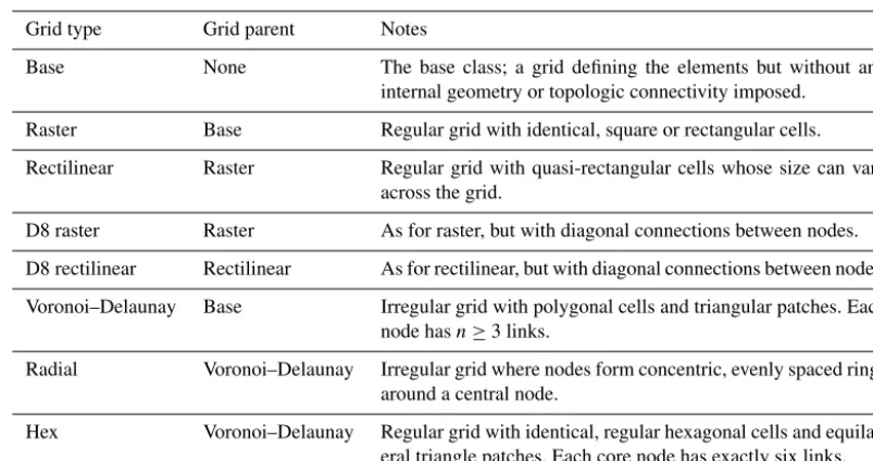
Table 2.Currently implemented grid types in Landlab.
Grid type Grid parent Notes
Base None The base class; a grid defining the elements but without any
internal geometry or topologic connectivity imposed.
Raster Base Regular grid with identical, square or rectangular cells.
Rectilinear Raster Regular grid with quasi-rectangular cells whose size can vary
across the grid.
D8 raster Raster As for raster, but with diagonal connections between nodes.
D8 rectilinear Rectilinear As for rectilinear, but with diagonal connections between nodes.
Voronoi–Delaunay Base Irregular grid with polygonal cells and triangular patches. Each
node hasn≥3 links.
Radial Voronoi–Delaunay Irregular grid where nodes form concentric, evenly spaced rings
around a central node.
Hex Voronoi–Delaunay Regular grid with identical, regular hexagonal cells and
equilat-eral triangle patches. Each core node has exactly six links.
Cell Node (core) Active Link Face
Inactive Link Node (open boundary)
Node (closed boundary)
Figure 5. Interplay of node and link boundary conditions on a Landlab example grid. Because nodes rather than corners define the outer margin of the grid structure, the perimeter nodes lack cells, and the perimeter links lack faces (see main text). These aberrant nodes and links are automatically set as boundary ele-ments. Landlab defaults to setting the condition of any such node to FIXED_VALUE_BOUNDARY and any such link to INACTIVE.
but also to the ordering of elements around other elements (such as links around a node), and to the ordering of grid edges where needed (i.e. the standard order is right, top, left, bottom edges). Simple ordering examples are illustrated in Fig. 4.
We extend this same rotational convention to define the di-rectionality of all linear elements (such as links and, where necessary, faces), when such directionality is required. The positive direction is associated with the top-right (first) quad-rant; in other words, the positive direction is the one that points more right than down or more up than left. This is shown in more detail in Fig. 4b. This kind of directionality is important for example in the definition of fluxes along links into and out of nodes. In the case of link directions, Landlab provides masking arrays that can describe the local orienta-tion of each link with respect to another feature; for instance,
link_dirs_at_nodedescribes whether a link points into (+1) or out of (−1) any given node. The use and utility of such data structures is illustrated in Sect. 5.
3.1.3 Mappings and grid characteristics
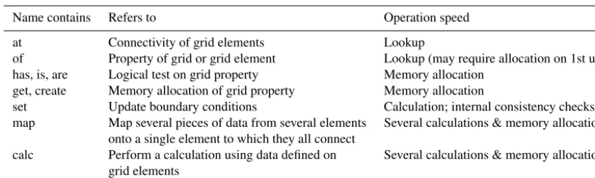
Landlab uses a standardized grammar to describe the meth-ods and Python properties in the grid classes that provide in-formation about the mapping of grid elements onto other el-ements, and to obtain information about the grid (e.g. areas, lengths, gradients). The intention of this standardization is to not only make it easier for users to quickly find the method they require but also provide information on the computa-tional efficiency of the operation. Some of this information is summarized in Table 3.
Grid characteristics
Landlab grids provide Python properties to describe the geometric characteristics of the elements them-selves, for instance position and dimension. These prop-erties are denoted by the preposition “of”, as in, for
Table 3.Standard grid method and property naming conventions, listed in approximate order of operation speed.
Name contains Refers to Operation speed
at Connectivity of grid elements Lookup
of Property of grid or grid element Lookup (may require allocation on 1st use)
has, is, are Logical test on grid property Memory allocation
get, create Memory allocation of grid property Memory allocation
set Update boundary conditions Calculation; internal consistency checks
map Map several pieces of data from several elements Several calculations & memory allocations onto a single element to which they all connect
calc Perform a calculation using data defined on Several calculations & memory allocations
grid elements
area_of_cell. Use of the wordoftells the user that an array of floats (or, more rarely, integers) denoting a grid characteristic is the expected return. (See for example use of angle_of_linkin Fig. 4b.)Ofis also used to access many counted characteristics of the grid as a whole, such as number_of_nodes. All these properties return pre-allocated arrays or single values already stored in memory, and can be expected to be fast.
Grid element mappings
The grid also provides numerous Python properties that describe the connectivity and associations of elements with one another. These are denoted by the preposition at.
Ex-amples include face_at_link, link_at_face,
links_at_node, patches_at_node, and
node_at_cell. Use of at tells the user that an array of element IDs is the expected return (see Fig. 4 for exam-ples of usage). The Landlab boundary condition interface
also uses at; for instance, status_at_node returns
an array containing the boundary condition status (as an integer code) of the grid nodes. All these properties return pre-allocated arrays, and can be expected to be fast.
“has”, “is”, and “are” methods
Use of has,is, or arein a method name indicates that the method in question applies a logical test to grid properties. These are not simple lookups, as in the case ofatandof prop-erties, but can still be expected to be fairly fast. The returned object will either be a Boolean or an array of Booleans.
Examples include is_boundary,are_all_core, and
has_field.
“get” and “create” methods
Landlab’s design philosophy seeks a balance between speed of access of information about the grid, and memory usage. To this end, only the most commonly used arrays of grid characteristics accessed by atandofproperties are created at grid instantiation. In other cases, these arrays are allocated
in memory at the first time of usage in code, then referenced from that point on at subsequent calls of the property. Meth-ods in the grid that begin withget or create are called by these properties the first time they themselves are used, and construct the necessary arrays in memory. These methods are typically intended for call only by a well-defined sub-set of other methods internal to grid, and not directly by the user; i.e. in programmer’s parlance they are “private”. We use the standard Python practice of beginning such methods with a leading underscore in the name, which tells the vari-ous Python user interfaces not to report them in standard lists of grid methods.
Computational methods
Landlab provides a large number of grid methods to allow easy completion of common and frequently repeated analy-ses of the values on the grid. These are denoted by names that begin withcalc, to denote methods that calculate a new value from provided data, ormap, which apply some standard rule to map multiple values for connected elements to a single value on the shared element to which they connect. For in-stance,calcmethods might allow calculation of gradients at links from data defined at nodes (calc_grad_at_link), or flux balances at a node from fluxes defined at
incom-ing and outgoincom-ing links (calc_flux_div_at_node).
Map methods might return means of values at links
around nodes (map_mean_of_links_to_node),
or minima of node values attached to each link
(map_min_of_link_nodes_to_link), or
the maximum slope of links leaving each node
(map_downwind_node_link_max_to_node). More complex mapping schemes are also available, to allow for instance the mapping of data from topographically
upwind or downwind elements only (for example, map_
Boundary condition control
Grid methods that allow user control of boundary conditions use the word “set”. Boundary condition handling is described further in Sect. 3.1.4, below.
General rules
Words are separated by single underscores. Nouns are typ-ically singular, both describing the element and its
char-acteristic, e.g. area_of_cell, not areas_of_cells.
The exceptions are cases in which more than one thing is
associated with each element, such as links_at_node,
faces_at_cell. Any grid property can be expected to be a fast lookup operation if called repeatedly; methods may re-quire additional memory allocation.
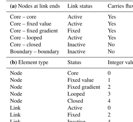
3.1.4 Grid boundary condition handling
Also provided are methods to facilitate boundary condition handling (Fig. 5). Nodes can have one of four boundary condition types:fixed value(Dirichlet),fixed gradient (Neu-mann), looped, or closed. A node that is not defined as a
boundary is known as a core node. The boundary
condi-tions defined on the nodes determine whether each connect-ing link is active(allows flux along it), fixed (allows flux, but flux value is fixed) or inactive (flux is forbidden), as shown in Table 4a. Each of these boundary conditions is associated with an integer value, which can be seen in the
boundary condition arrays grid.status_at_nodeand
grid.status_at_link(Table 4b).
We should emphasize that this framework is provided for user’s convenience; it can be easily ignored if a user wishes to implement a different scheme for boundary condition han-dling. Further, the appropriate boundary conditions depend on the physical scenario that the user is modelling.
The edges of a Landlab grid are always defined by bound-ary nodes. Because perimeter nodes lack cells (Sect. 3.1.1), this means not every boundary node necessarily has a cell, and may also not have the standard number of links, patches, etc. (Table 1b). Conversely, any core node can always be ex-pected to have a cell and a standard connectivity as described in that table. Likewise, inactive links at the grid perime-ter lack faces, but each active link always inperime-tersects, and is uniquely associated with, a single face (Fig. 5). Thus, cells share the boundary conditions of nodes (core vs. boundary) and faces share the boundary conditions of links (active vs. inactive). Note also that nodes that are in the interior of a grid (i.e. not perimeter nodes) can also be assigned as bound-ary nodes, and that whether or not this occurs depends on the shape of the area that the user is modelling. For exam-ple, a user may wish use a grid that represents a drainage basin, with the basin’s interior consisting of core nodes, a single node representing the outlet (flagged as a fixed-value or fixed-gradient boundary), and the remainder of the nodes flagged as closed boundaries.
Table 4.(a)Link boundary condition status as dictated by node boundary condition status.(b)Integer values associated with each boundary condition status.
(a)Nodes at link ends Link status Carries flux?
Core – core Active Yes
Core – fixed value Active Yes
Core – fixed gradient Fixed Yes
Core – looped Active Yes
Core – closed Inactive No
Boundary – boundary Inactive No
(b)Element type Status Integer value
Node Core 0
Node Fixed value 1
Node Fixed gradient 2
Node Looped 3
Node Closed 4
Link Active 0
Link Fixed 2
Link Inactive 4
The grid itself is responsible for keeping track of and ensuring internal consistency between boundary condition properties. The standard numpy setters and getters are over-ridden for the boundary condition data structures to ensure this internal consistency without the user’s involvement. For example, if a user changes a node’s status from core to fixed-value boundary, the gridding engine will automatically up-date the status of the relevant links.
3.2 Spatially distributed data and data fields
A key element of any model of surface processes is a de-scription of how the state variables and surface character-istics vary across the domain. Such data can include both scalar measurements at a point or over an area (such as to-pographic elevation, water depth, sediment cover fraction, vegetation type) and directional vector data, for instance, de-scribing fluxes across the surface or gradients in scalar val-ues. Landlab uses data constructs calleddata fieldswithin the grid to store and handle this information.
links describe the connectivity between nodes, vector infor-mation describing fluxes or gradients between nodes is read-ily stored on links; the link’s orientation provides an implied unit vector, while the associated value represents the vector’s magnitude. There are also a number of use cases in which values can usefully be stored on patches, for instance, in rep-resenting resolved means of vector values at the bounding links. This data structure also lends itself to the implementa-tion of some cellular automata. For instance, pairwise transi-tion automata (Narteau et al., 2001, 2009) represent the states of cells on a grid as paired “doublets”, with rules prescribed to govern the rates of transition between each doublet type. These are readily implemented in Landlab by mapping the pair states onto the links of a Landlab grid, and representing the corresponding automaton cell states at grid nodes (Tucker et al., 2016).
In terms of implementation in the code, Landlab fields are represented as a dictionary of Python dictionaries within the grid object. The keys to the first dictionary are strings of the names of the grid elements (viz., “node”, “link”, “patch”, “cell”, “face”, “corner”); the keys to the dictionaries that these return are Landlabfield names. Users are free to cre-ate field names as they wish. However, Landlab maintains a standard format and name list which is widely used by the Landlab component library (Table S1 in the Supplement), and users are strongly encouraged to adopt this scheme to enhance standardization and interoperability throughout the software. Our standard naming scheme echoes that of the community standards adopted by the Community Surface Dynamics Modeling System (CSDMS). Our rationale fol-lows theirs, aiming to remove ambiguity in the identifica-tion of different types of numerical informaidentifica-tion (Peckham, 2014; Peckham et al., 2013). However, given the potential for high frequency of name usage in Landlab code, and our ability to easily assess potential ambiguities between differ-ent compondiffer-ents, we place more value on name brevity at the expense of total unambiguity as compared with the for-mal CSDMS Standard Names (https://csdms.colorado.edu/ wiki/CSN_Searchable_List). Nonetheless, we maintain one-to-one mappings with the CSDMS Standard Names to en-able automated implementation of the CSDMS Basic Model Interface (BMI; see Sect. 3.4.1).
The general format for Landlab names is
“thing_described__quantity_described”. This approach
is more generally known as the object–attribute–value paradigm: the first word or phrase describes the object, the second word or phrase describes the attribute, and the variable’s content is its value. A double underscore separates the object from the attribute. An example might be “surface_water__discharge”. A full list of names used in Landlab components as of version 1.0 can be found in the Supplement as Table S1. A version of this list up to date with the current release version can be found on the Landlab website.
Units can be attached to grid fields. They are recorded in a further dictionary-like structure, which is a property of the element container. This means they can be accessed with
syn-tax likegrid['node'].units['field__name'].
Landlab offers some degree of “syntactic sugar” for its field name interface – i.e. the field interface is made more user-friendly by the addition of more readable grid prop-erties to query the fields at each element type, rather than requiring the user to access the both dictionaries directly.
For instance, grid.at_node['my_field_name']is
equivalent to grid['node']['my_field_name'].
In addition, Landlab also provides convenient
short-cuts to create new fields of ones (grid.add_ones),
zeros (grid.add_zeros), and from existing data
(grid.add_field).
3.3 Components
Components are Python objects that simulate processes within Landlab. A typical Landlab component provides a nu-merical representation of a single process. For instance, a component might compute the flow of water across a terrain surface using a particular flow law and numerical solution method. Components also exist in Landlab that produce only spatially invariant time series, or that produce time-invariant steady-state solutions across a surface. A prominent example would be the FlowRouter component, which calculates the steady-state accumulation of water discharge and upstream total drainage area through a drainage basin. The latter cate-gory also includes a number of analytical tools that produce spatial statistics for a surface; for example, components to calculate the steepness (Wobus et al., 2006) or chi index (Per-ron and Royden, 2012) for a channel network.
Multiple components can be used together, allowing the simulation of multiple processes acting on a single grid. For example, components simulating hillslope processes and flu-vial geomorphic processes can be easily implemented to-gether to create a “custom” landscape evolution model. In some cases, the output from one component may form the input to another, as for example when combining flow rout-ing and sediment transport components, or soil moisture and vegetation growth components. The design of each compo-nent is intended to work in a “plug-and-play” fashion, where each component couples simply and quickly to others. This is permitted by a standardized interface for each component, as described in Sect. 3.3.1. Examples of coupled component systems can be seen in Sect. 5.
Land-lab, for the use of others. Documentation and advice for this process can be found on the Landlab website.
3.3.1 Component standard interface
Landlab components have standardized interfaces, which are designed to enhance interoperability both internally to lab (between components, or between components and Land-lab utilities) and between LandLand-lab and external interfaces like the CSDMS Basic Model Interface (Peckham et al., 2013) (see also Sect. 3.4.1). The Landlab standardized component interface consists of the following:
– An initialization method, with the standard argument
signature __init__(self, grid, x=a, y=b,
z=c, ..., ∗∗kwds), where gridis a Landlab grid object;x,y, andzare component-specific keyword ar-guments with default values a, b, and c; and ∗∗kwds
is an optional keyword argument dictionary. The grid object passed during instantiation is accessed during the running of the component, and its data fields are updated automatically. A component may have any number of component-specific keyword arguments. The variable names of these arguments are not standard-ized but rather generally unique to each component. The component-specific arguments are, however, required to have default values. The names of the keyword argu-ments make explicit the data requireargu-ments of the com-ponent in order to run. However, the∗∗kwdsargument alternatively allows these parameters to be set from a dictionary of model parameters. In other words, this component could be initialized in two equivalent ways:
>>> ld = LinearDiffuser(grid, linear_diffusivity=1.0,
method='simple')
or
>>> paramdict = {
'linear_diffusivity': 1.0, 'method': 'simple'}
>>> ld = LinearDiffusivity(grid, **paramdict)
– A run method, with the standard argument signature
run_one_step(dt, ∗args, ∗∗kwds), wheredt
is an interval of time over which to execute the compo-nent before returning a result, and∗argsand∗∗kwdsare an argument list and dictionary respectively, specific to each component. These latter items allow any additional arguments necessary for the model to run to be passed in. Ifdtis not required for a component to run, it may be omitted.
– A standard set of properties for the component:
name,input_var_names,output_var_names,var_units,
var_mapping, andvar_definition. These properties de-scribe the fields that the component interacts with, the units of each, which element each field is defined on, and a brief summary of what each field represents.
All components inherit from the base classComponent. This base class enables and regulates the standardized prop-erties and interface that are available for every Landlab com-ponent. It also provides methods designed to streamline the creation of the output data fields when a component is instan-tiated.
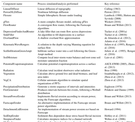
Landlab version 1.0 provides a standard component library as part of its installation. A full list of components available in version 1.0 can be found in Table 5. Although these ex-isting components are largely Earth-surface focused, we em-phasize that Landlab permits modelling of the evolution of almost any two-dimensional system that lends itself to de-scription by discretized systems of differential equations or cellular automaton rules.
3.3.2 Timestepping and interaction of components
For most existing Landlab components, the component is re-sponsible for controlling its own internal numerical stabil-ity. A timestep parameter dtis passed to each component that operates in a time-dependent fashion; this timestep can be thought of as the “coupling timescale”, and it represents the frequency of interaction between components if more than one is coupled (Fig. 6). However, it is not necessarily the stable timescale, which will vary between components. Each component is responsible for calculating its own stable timestep under the model run conditions, and internally sub-dividing the imposeddtin order to ensure the model run does not become unstable. The user is responsible for selecting an appropriate coupling timescale – too short, and a model run will take more steps than necessary for each component to be stable; too large, and information transfer between the com-ponents will be limited, possibly introducing an additional source of numerical error.
Table 5.Components available in Landlab v.1.0.
Component name Process simulated/analysis performed Key reference
LinearDiffuser Linear diffusion of topography Culling (1963)
PerronNLDiffuse Nonlinear hillslope diffusion Perron (2011)
Flexure Simple lithospheric flexure under loading Lambeck (1988), Hutton and
Syvitski (2008)
gFlex A more complex flexure model, utilizing gFlex Wickert (2016)
FlowRouter A convergent flow router, following the Fastscape
algorithms
Braun and Willett (2013)
DepressionFinderAndRouter A lake filler that can route flow across depressions Tucker et al. (2001a)
SinkFiller An algorithm to fill depressions in a surface Tucker et al. (2001b)
OverlandFlow A shallow overland flow approximation de Almeida et al. (2012),
Adams et al. (2016) KinematicWaveRengers A solution to the depth varying Manning equation for
surface flow
Julien et al. (1995), Rengers et al. (2016)
SoilInfiltrationGreenAmpt Infiltrate surface water into a soil following the Green– Ampt method
Julien et al. (1995), Rengers et al. (2016)
SoilMoisture Compute local inter-storm water balance and root-zone soil
moisture saturation fraction
Laio et al. (2001)
PotentialEvapotranspiration Calculate potential evapotranspiration across a surface ASCE-EWRI (2005), Zhou et al. (2013)
Radiation Calculate total incident shortwave solar radiation Bras (1990)
Vegetation Calculate above-ground live and dead biomass, and leaf
area index
Istanbulluoglu et al. (2012), Zhou et al. (2013)
VegCA Cellular automata algorithm to simulate spatial
organization of PFTs
Zhou et al. (2013)
PrecipitationDistribution Generate a storm sequence of intervals and intensities Eagleson (1978)
FireGenerator Produces intervals between fire events, following a Weibull
distribution
Polakow and Dunne (1999)
StreamPowerEroder Implements fluvial erosion according to stream power,
using the Fastscape algorithms
Braun and Willett (2013)
FastscapeEroder An alternative implementation of the Fastscape stream
power algorithms
Braun and Willett (2013)
DetachmentLtdErosion An implementation of stream power erosionnotbased on Fastscape
Howard (1994)
SedDepEroder Sediment-flux-dependent shear stress based fluvial incision Hobley et al. (2011)
SteepnessFinder Calculates steepness indices for a channel network Wobus et al. (2006)
ChiFinder Calculates the chi index along a channel network Perron and Royden (2012)
is assumed to have read the component documentation and taken on board that this is potentially an issue, as well as taken steps to check that their output is behaving sensibly and is not highly sensitive to changes in the supplied timestep. We reiterate that it is ultimately the user’s responsibility to check that the provided dt is appropriate to the modelling scenario at hand.
3.3.3 Parallelization
Together, the componentized nature of Landlab and the level of flexibility afforded to the user conspire to rule out the idea of Landlab as a whole being highly optimized through paral-lelization. However, there is great potential for parallelization of Landlab at the component level, since the run methods of each component are entirely self-contained. As proof of
con-cept, the Flexure component has already been parallelized (see online code and documentation). Although in Landlab version 1.0 we have not had a compelling enough use case to invest significant time in such work, many of the components already in the library would be amenable to parallelization in this style, and this could be done in future releases.
3.4 Utilities and interfaces
for-Driver imposed timestep, dt
Component 1, stable timestep dt1
Component 2, stable timestep dt2 = dt1
Component 3, stable timestep dt3 > dt
Component 4, unconditionally stable
dt
dt1
dt2
dt3
Information exchange Information exchange Information exchange
Time passing
Figure 6.Interaction of timescales between a Landlab driver and a set of components. In this example, a driver that implements com-ponents 1–4 has a time loop of lengthdt, anddtis the timescale that is passed to the components. Components 1 and 2 implement nu-merical schemes that have maximum stable timesteps shorter than
dt. In these cases, the imposeddtinterval is internally subdivided to ensure the model remains stable. Here, we see two possible ways a component might do this, either always taking the largest timestep possible then a short timestep to finish (component 1) or by divid-ing the imposed timestep into the minimum number of equal length internal steps,dtint, wheredtint<dtstable(component 2). Even if a
component could run for a timestep longer than dt (e.g. compo-nents 3 and 4), under an explicit-time Landlab driver script like this, its steps will be truncated atdt. Once all the components have run fordt, they sequentially update their output fields in the grid with their changes. This is the only time that information can be passed actively between each component (and the driving script, if it also makes changes to the grid fields within the loop); each component cannot “feel” changes being made by any other untildthas elapsed. Hencedtis best thought of as the “coupling timescale”.
mats. These options are intended to allow interoperability with third-party software, especially geographical informa-tion systems, and also to allow Landlab data to be manipu-lated in and displayed with specialized visualization software (such as ParaView).
Landlab’s standard interfaces also allow it to interact more easily with software frameworks developed by the geo-science and hydrogeo-science communities. For instance, Land-lab is already embedded within the Hydroshare colLand-labo- collabo-ration environment, http://www.hydroshare.org. This means that Landlab models can be created and run within the Hy-droshare data and modelling environment and can take ad-vantage of that environment’s shared data platform and meta-data systems.
3.4.1 Dynamic model interaction and the Basic Model Interface
As noted in previous sections, Landlab has been designed from conception to be fully compliant with the Community Surface Dynamics Modelling System’s Basic Model Inter-face (BMI) (Peckham et al., 2013). The BMI concept al-lows any two models describing the changes caused by sur-face processes to be coupled together, regardless of the va-garies of model gridding schemes, programming languages, or other low-level design choices. It does this by means of a standard interface (the Basic Model Interface, sensu stricto), which is callable for any BMI compliant model or component and includes generically applicable functions
such as initialize, update (i.e. run one timestep),
andget_current_time. The interface allows informa-tion about the current state of a simulainforma-tion to be passed back and forth between running models in a manner that is agnos-tic in terms of implementation details.
The Landlab framework is designed such that the Land-lab standard component interface can also expose a full BMI interface; in other words,all Landlab components are also BMI-compliant components. This means that by choosing Landlab as their model development environment, users also gain the ability to couple their models immediately with any other model in the CSDMS repository of BMI-compliant codes. This choice will also enhance the utility of Landlab to users who wish to implement component functionality along-side some other model using the CSDMS BMI or Web Mod-eling Tool (WMT) (Piper et al., 2015).
4 Validation, testing, and documentation
Landlab also includes suites of unit tests. These are test scripts written specifically to exercise particular aspects of the code, and to check the output of that test against known correct solutions. Examples of when this is useful can occur in longer or more involved code, especially in components, where various different configurations of grid types and ini-tial and boundary conditions need to be tested to ensure the component is robust under various different conditions. Unit tests differ from doctests in that they are not intended to be user-facing, although they are run alongside them when test-ing of the code base is triggered.
Almost all core Landlab functionality of both grid meth-ods and components is now tested in this way. As of this version, around 1400 separate tests are run on the code each time testing is triggered, and the tests cover 80 % of the code base. Most of the remaining uncovered code is either chal-lenging to adequately test (for example, plotting functions), not part of the core Landlab functionality (such as helper scripts involved in building releases), or deprecated. Tests are triggered automatically and remotely through the web-based applications Travis (Mac/Linux) and Appveyor (PC) whenever a new commit is made to either a branch or the master version of the code repository on GitHub, or when a new release of the code is built. These tests are performed on a range of supported Python versions, including both ver-sions 2 and 3. Tests can also be triggered manually on a local machine by running a testing script included with Landlab, or
by calling landlab.test()from an interactive Python
environment.
5 Creating models with Landlab
We here illustrate some of the key functionality of Landlab by example, demonstrating its applicability across a variety of types of problem. We hope to emphasize here that Land-lab is not a landscape evolution model(although it can be used to create them) – rather, it presents a framework under which a wide variety of different models can be implemented using its tools, including hydrologic, ecologic, and sedimen-tological models, as well as landscape evolution models. This section illustrates four possible contrasting model designs that can be implemented within the Landlab framework: a very simple “toy” geomorphic diffusion code that demon-strates the core functionality of the grid; a coupled stream power–hillslope diffusion model driven with a stochastic se-quence of storms, illustrating some of Landlab’s compo-nents; a cellular automaton, demonstrating a fundamentally different style of model implementation that is also enabled by Landlab’s design; and a flood wave routing model, run on real topographic data ingested by Landlab. We hope that these examples will also serve as an illustration of the po-tential power of the Landlab framework to enable novel or under-explored process interaction studies (e.g. of vegetation
on landscape evolution; of surface hydrology on stochastic surface processes).
5.1 A simple diffusion model
Although Landlab provides “off the shelf” process simula-tion code in the form of the components, Landlab also facil-itates the design of models without using the components. The Landlab grids provide mapping, gradient, and diver-gence functions to make implementation of, for instance, finite-difference or finite-volume methods both concise and straightforward.
Here we illustrate this functionality using a simple finite-volume diffusion scheme, which here is representing the downslope flow of soil on hillslopes (Culling, 1963). We wish to represent the evolving form of a diffusional hillslope that is undergoing a constant uplift (1 mm yr−1) with refer-ence to a relative base level. In this case, the grid is radial and so roughly circular in plan view. Use of this particular configuration is intended in part to demonstrate the flexibil-ity of Landlab’s design, although this radial grid arrangement could perhaps be thought of in terms of response to a rising volcanic mound or salt diapir or another similar scenario with a radially symmetric uplift field.
The governing equations for this example are
∂η
∂t =U− ∇qs, (1)
qs= −D∇η, (2)
whereηis land-surface elevation,t is time,Uis the rate of vertical motion (“uplift”) of rock relative to base level,qsis
volumetric sediment flux per unit slope width, andD is a transport coefficient with dimensions of length squared per time.
For our example model, Eq. (2) will be discretized and solved using a finite-volume solution scheme. Consider a cell of surface areaathat is surrounded byNneighbouring cells (Fig. 7). We can integrate Eq. (1) over the surface area of the cell:
Z
a
∂η ∂tda=
Z
a
Uda−
Z
a
∇qsda. (3)
Applying the divergence theorem to the last term on the right, and evaluating the other two integrals,
a∂η
∂t =U a−
I
p
qs(p)ndp, (4)
12 11
17
7
13
19
15
20 24
52
50 48
51
47 SOIL
SOIL SOIL
SOIL
SOIL SOIL
SOIL SOIL
Calculating gradients at links:
>>> grad = grid.calc_grad_at_link(elev) >>> grid.links_at_node[12]
array([20, 24, 19, 15])
>>> grad[grid.links_at_node[12]] array([-0.2, 0.2, -0.1, 0.3])
Calculating fluxes from gradients:
>>> q = -0.01 * grad >>> q[20]
0.002 >>> q[15] -0.003
Calculating flux divergence:
>>> divq = grid.calc_flux_div_at_node(q) >>> divq[12]
0.0002
Node spacing = 10 m
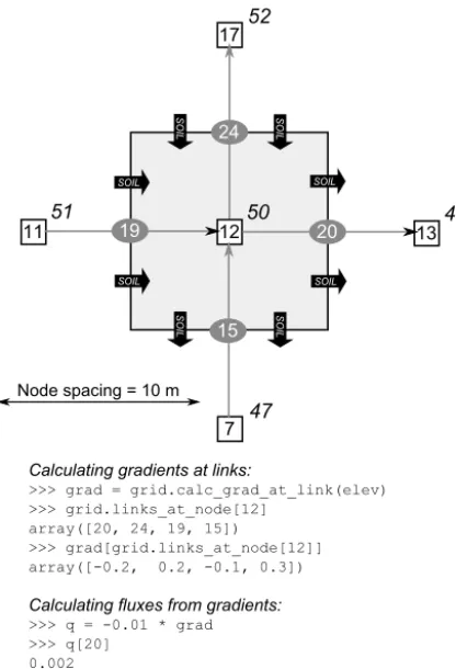
Figure 7.Schematic illustration showing how Landlab’s grid ge-ometry may be used to construct a finite-volume numerical scheme. White squares represent nodes, with example node IDs given for a 5×5 raster grid. Grey ovals show the centre points of the links, with the link IDs given. In this example, we assume that we have a node field called “elev” whose values represent the altitude of the land surface at various node locations (example values shown in italics next to each node). Black arrows indicate direction of soil flow (in the downhill direction). A finite-volume solution for a dif-fusion model can be implemented by (1) calculating the gradient at each pair of adjacent nodes and assigning it to the correspond-ing link (lines 1–3 in the code snippet below); (2) multiplycorrespond-ing by a transport-rate coefficient (and−1) to obtain unit flux (lines 4–6); and (3) multiplying the unit flux at each cell face by the width of that face, adding up the inflows and outflows, and dividing by cell area to obtain flux divergence (lines 7 and 8).
polygon with N faces, this last term can be replaced by a summation:
∂η ∂t =U−
1
a
N
X
k=1
qskwk (5)
whereqskis the unit flux at facek, positive outward, andwk
is the width of facek.
We will implement this solution in Landlab by assigning to each nodeithe value of the average elevation within its cell,ηi (for notational convenience, we will drop the use of
the overbar below). To calculate the flux at each face, we first need to calculate the topographic gradient at each face. We will do this by taking the elevation difference between each neighbouring pair of nodes, dividing by the length of the link that connects them, and then assigning the resulting gradient value to the relevant link. The gradient at linkj is therefore calculated as
Gj=
ηHj−ηTj
Lj
, (6)
whereηHj andηTj are the elevation values at linkj’s head
and tail nodes, respectively, andLj is the length of linkj.
In Landlab’s gridding engine, the calculation of link-based gradients in a node-based scalar quantity likeηis handled
by the grid methodcalc_grad_at_link, which takes a
node array or field name as an argument and returns a link ar-ray. Figure 7 illustrates how values ofηdefined at nodes can be used to calculate gradients at links, and then the gradients can be used to calculate the net flux into and out of a cell.
In our diffusion example, the summation of fluxes along the cell faces is calculated as follows:
N
X
k=1
qskwk=
D ai
N
X
k=1
δikGkwk, (7)
whereδikindicates the direction of linkkrelative to the cell
i: ifδik= −1, the link points outward from the cell; ifδik= +1, the link points inward.
To calculate flux divergence using this finite-volume approach, Landlab provides the general grid method
calc_flux_div_at_node, which takes a link-based ar-ray of unit fluxes as an input and returns a node arar-ray that contains the sum of in/out fluxes (divided by cell area) at each node (Fig. 7). Values at perimeter nodes, which lack cells, are ignored. In keeping with the standard definition of the divergence operation, the function returns positive values where the net flux is outward and negative values where it is inward.
In the diffusion example shown in Fig. 8, the time deriva-tive is discretized using a simple forward-Euler explicit method, such that the values of elevation at the new timestep
t+1 are calculated from values at the old timestep:
ηit+1=ηit+1t
"
U+D ai
N
X
k=1
δikGkwk
#
, (8)
where the superscript indicates timestep, and the
quantity in brackets is evaluated at timestep t. The
code to implement the model is shown in Fig. 8. Note the use of the calc_grad_at_link and
1. >>> from landlab import RadialModelGrid, imshow_grid 2. >>> from matplotlib.pyplot import show
3. >>> mg = RadialModelGrid(num_shells=10, dr=10.) 4. >>> z = mg.zeros('node')
5. >>> qs = mg.zeros('link') 6. >>> diffusivity = 1.e-2
7. >>> dt = 0.2 * mg.length_of_link.min() ** 2. / diffusivity 8. >>> for i in range(500):
9. ... z[mg.core_nodes] += 0.001*dt 10. ... g = mg.calc_grad_at_link(z)
11. ... qs[mg.active_links] = -diffusivity * g[mg.active_links] 12. ... dqsdx = mg.calc_flux_div_at_node(qs)
13. ... dzdt = -dqsdx
14. ... z[mg.core_nodes] += dzdt[mg.core_nodes] * dt
15. >>> imshow_grid(mg, z, grid_units=('m', 'm'), var_name='Elevation (m)') 16. >>> show()
100 50 0 50 100
X (m) 100
50 0 50 100
Y (m)
0 25 50 75 100 125 150 175 200 225
Elevation (m)
Code to implement a simple diffusion model on a radial Landlab grid:
Figure 8.A simple finite-volume hillslope diffusion model imple-mented in Landlab. Values adopted here are within typical terres-trial ranges for hillslope length (∼100 m, controlled from line 3), hillslope diffusivity (0.01 m2yr−1, line 6) (Fernandes and Diet-rich, 1997), total time of run (around a million years, since dt
is ∼1833 years, lines 7–8), and uplift rate relative to base level (0.001 m yr−1, line 9).
An advantage of the finite-volume approach is that it can be applied to cells of any shape. For instance, it can be used with hexagonal cells, or with Voronoi polygons as in the ex-ample in Fig. 8.
This model can be implemented in Landlab and plotted in as few as 16 lines of code (Fig. 8). Here, line 1 imports the Landlab classes and functions we will use, and line 2 imports theshow()function from matplotlib that will let us display the plot. Line 3 instantiates the Landlab grid object. This example uses a RadialModelGrid, but the same code would work with any grid type. Lines 4–6 initialize data for the model run. zwill be the land surface elevation at each node;qswill be the volumetric sediment flux per unit width along each link. Note that this implementation is consciously not using data stored as Landlab fields in order to illustrate that this is not a requirement; however, it would be trivial to modify lines 4 and 5 to create the data as fields on the grid, and the remainder of this script would be unchanged. Line 7 is the first line that actually begins the calculations that perform the diffusion. This line calculates a Courant– Friedrichs–Lewy (CFL) stability condition (Slingerland and Kump, 2011) for the maximum stable timestep for the finite-volume scheme we are about to implement.
1. >>> from landlab import RadialModelGrid, imshow_grid 2. >>> from landlab.components import LinearDiffuser 3. >>> from matplotlib.pyplot import show
4. >>> mg = RadialModelGrid(num_shells=10, dr=10.) 5. >>> z = mg.add_zeros('node', 'topographic__elevation') 6. >>> dt = 2000. # no longer the stable timestep 7. >>> ld = LinearDiffuser(mg, linear_diffusivity=1.e-2) 8. >>> for i in range(500):
9. ... z[mg.core_nodes] += 0.001*dt 10. ... ld.run_one_step(dt)
11. >>> imshow_grid(mg, z, grid_units=('m', 'm'), var_name='Elevation (m)') 12. >>> show()
Code to implement a simple diffusion model on a radial Landlab grid, using Landlab components:
Figure 9.Hillslope diffusion implemented in Landlab using a com-ponent. Compare to Fig. 8. Note that this version is more concise, and that timestep stability is now handled internally within the com-ponent.
Lines 8–14 implement a time loop, within which the dif-fusion occurs. The core (i.e. interior) nodes of the grid are uplifted at a rate of 0.001 length units per time unit relative to base level. Lines 10–14 implement the meat of the differ-encing scheme, where we use a staggered grid to solve the discretized diffusion equation (Eq. 8). The depth-integrated fluxes on the links are calculated as the product of the diffu-sivity parameterDand the topographic gradient at the links (lines 10, 11), taking care to calculate the flux only on ac-tive links. The flux divergence is then calculated at each node based on the fluxes on the links to which is it adjoined (line 12). Note that Landlab enables each of these operations to be performed with a single grid method. The final lines of the code invoke the standard Landlab plotter, then display the output. Although we have not specified any particular units in our calculation, in line 15 we assert that the length unit is metres and the time unit is years.
Note that this same result could have been achieved even more concisely using Landlab’s in-built LinearDiffuser com-ponent. The equivalent code is shown in Fig. 9. Not only are the implementation details of the scheme now handled entirely within the component, but so also is internal sub-division of the provided timestep to meet the necessary sta-bility conditions for the simulation. Additionally, the eleva-tion data are now passed into the component as the field “topographic__elevation” – which is attached to the grid – rather than as a separate variable (lines 5, 7), as discussed in Sect. 3.2.
5.2 Coupling diffusion to stream power with a storm sequence