Robust optimization methodologies for water supply systems design

Drink. Water Eng. Sci., 5, 31–37, 2012 www.drink-water-eng-sci.net/5/31/2012/ doi:10.5194/dwes-5-31-2012

©Author(s) 2012. CC Attribution 3.0 License.

History

of

Geo- and Space

Sciences

Open

Access

Advances

in

Science & Research

Drinking Water

Engineering and Science Open Access

Open

Access

Earth System

Science

Data

Drinking Water

Engineering and Science Discussions

O

pen

Acc

es

s

Open

Access

Earth System

Science

Data

D

iscussions

Robust optimization methodologies for water supply

systems design

J. Marques1, M. C. Cunha1, J. Sousa2, and D. Savi´c3

1_{Departamento de Engenharia Civil, Faculdade de Ciˆencias e Tecnologia da Universidade de Coimbra, Portugal} 2_{Departamento de Engenharia Civil, Instituto Superior de Engenharia de Coimbra, Portugal}

3_{Centre for Water Systems, School of Engineering, Computing and Mathematics, University of Exeter, UK}

Correspondence to: J. Marques ([email protected])

Received: 26 March 2012 – Published in Drink. Water Eng. Sci. Discuss.: 18 April 2012 Revised: 9 July 2012 – Accepted: 9 August 2012 – Published: 15 August 2012

Abstract. Water supply systems (WSSs) are vital infrastructures for the well-being of people today. To

achieve good customer satisfaction the water supply service must always be able to meet people’s needs, in terms of both quantity and quality. But unpredictable extreme conditions can cause severe damage to WSSs and lead to poorer levels of service or even to their failure. Operators dealing with a system’s day-to-day op-eration know that events like burst water mains can compromise the functioning of all or part of a system. To increase a system’s reliability, therefore, designs should take into account operating conditions other than nor-mal ones. Recent approaches based on robust optimization can be used to solve optimization problems which involve uncertainty and can find designs which are able to cope with a range of operating conditions. This paper presents a robust optimization model for the optimal design of water supply systems operating under different circumstances. The model presented here uses a hydraulic simulator linked to an optimizer based on a simulated annealing heuristic. The results show that robustness can be included in several ways for varying levels reliability and that it leads to more reliable designs for only small cost increases.

1 Introduction

Modern societies are sustained by a number of vital net-works. Energy, telecommunications, transport, water and sanitary infrastructures are responsible for a good quality of life. A disruption in the water supply can cause enormous trouble, which means that the systems have to be designed to deliver a constant supply of clean, safe drinking water, even in adverse circumstances. Every WSS will certainly have to contend with some burst pipes and abnormal demands, such as from firefighting. These events can have a minor or major impact on the operation of the WSSs and it is very impor-tant to maintain the supply and quality of water. According to DIEDE and AIDIS (2008), studies of hundreds of disasters worldwide clearly indicate that continuity of drinking water and sanitation services is critical in post-disaster conditions, since they are essential to rapid social and productive recov-ery. Water can still be provided, even in adverse situations, if a proactive attitude is taken towards risk from the design

phase until the end of the system’s life span. However, it must be pointed out that if all the possible threats and vulnera-bilities could be taken into account the cost would be pro-hibitive. Hence, decision makers must establish how much they are willing to pay to reduce risk. As a WSS is a costly infrastructure its design and operation should be supported by optimization tools. Stochastic optimization and robust op-timization (RO) appear to be promising techniques to solve these problems: the review by Mulvey et al. (1995) examines this area and describes some practical applications. RO has already been applied to WSS: Babayan et al. (2007), Jeong et al. (2006), Cunha and Sousa (2010), Carr et al. (2006) and Giustolisi et al. (2009) present a number of robust optimiza-tion models.

abnormal working conditions like firefighting flows and pipe breaks. This approach also considers two levels of pressure: the desired pressure (minimum pressure to meet water de-mand) and the admissible pressure (minimum pressure al-lowed for the abnormal conditions scenarios). The pressure for the peak discharge design scenario is always higher than the desired pressure and so the network must be designed to meet the water demand under normal working conditions. The pressure for the abnormal scenarios is allowed to take lower values, although they are always higher than the ad-missible pressure. However, if the pressure is lower than the desired pressure then part of the water demand will not be met and the objective function is penalized.

The solutions obtained with this method showed that a ro-bust design, a design that will meet all the desired pressure requirements even under abnormal working conditions, can be considerably more expensive than the traditional design solution (peak discharge design). As the case study used in Cunha and Sousa (2009) was a gravity fed water distribution network, the pipe diameters had to be increased to meet the pressure conditions in all scenarios, and consequently this added to the cost. For example, if the water demand is to be fully met during a pipe bursts the flow needs alternative paths to reach the demand nodes downstream of the break, and those paths must have enough capacity to carry a discharge that is higher than usual. As the pipe cost increases signifi-cantly with the diameter, this additional capacity is quite ex-pensive. It must also be pointed out that larger diameters lead to low velocities and high water residence times, neither of which are desirable in terms of water quality and safety.

This paper proposes a different approach. As larger pipe diameters significantly increase the cost and lead to low ve-locities, it might be possible to cope with abnormal working conditions, which occur sporadically and last a short time, by adding a pumping station to be used like a contingency infrastructure. The strategy of this work involves a gravity fed network design to cater at least for normal working con-ditions (peak design flow) and a pumping station to add en-ergy to cope with abnormal working conditions. The pump-ing station will only be planned to operate under abnormal working conditions, so the energy consumption can be ne-glected. It was also taken that the pressure under abnormal working conditions could be higher than under normal work-ing conditions, but never above a maximum pressure con-straint introduced in the optimization model. This will limit the elevation of the pumping station in abnormal conditions only to safe levels of operation.

With this contingency infrastructure, the network does not need to be overdesigned to attain the desired robustness, and this reduces the complications that can arise from low ve-locity problems. It can also be viewed as another way to in-crease robustness in an existing WSS where solutions such as increasing the pipe diameters may be hard to implement in an urban environment.

The optimization model is presented next, in Sect. 2, then the model is tested on 2 case studies in Sect. 3 and the re-sults and comparisons are presented in Sect. 4. Finally, the conclusions are set out in Sect. 5.

2 Robust model

The model proposed here is based on the work by Cunha and Sousa (2009) and is used for the robust design of WSSs ex-posed to different operating scenarios. But a new approach to achieving the desired robustness is considered now, one which uses a pumping station instead of increasing the pipe diameters. The goal of the model is to find designs that will perform well even under abnormal conditions (pipe breaks or firefighting). The optimization model is solved by the simulated annealing algorithm proposed in Aarts and Ko-rst (1989), used by Cunha and Sousa (1999) and Cunha and Sousa (2001) and adapted for this work. The model is linked to a hydraulic simulator that verifies the hydraulic con-straints. An hydraulic simulator based on a pressure driven approach is used to verify the hydraulic constraints. Consid-ering the sum of probabilities of all the scenarios to be 1, the objective function is formulated in Eq. (1):

Min

NPI P

i=1

Cpipei(Di)Li+

NPU P

j=1

CCpsj+CEpsj

+NSP

s₌1

prob_s "

Cpenp·

NN P

n₌1

max_{0; PMINdes}

s−Pn,s

2

+Cpend·

NN P

n=1

max_{0; QD}

n,s−QCn,s

2#_.

(1)

Where CCpsjis the construction cost and CEpsjthe

equip-ment cost in€of the pumping station (PS) j:

CCps_j=39 904+374×Qps_j+0.15×Qps_j

×Hps_j∀j∈NPU, (2)

CEps_j=1317×Qps0_j.769×Hps0_j.184+2092

×(Qps_j×Hps_j)0.466∀j∈NPU. (3) The objective function Eq. (1) includes the following costs: cost of the pipes and cost of the pumping stations (construc-tion and equipment). But it also includes a penalty func(construc-tion for those solutions that do not meet the minimum desired pressure and demands: the sum of the quadratic violations of pressures and demands multiplied by penalty coefficients and weighted by the probability of occurrence of each scenario.

The model includes a different set of constraints. Equa-tion (4) is used to verify the nodal continuity equaEqua-tions; Eq. (5) is used to compute the head loss of the pipes; Eq. (6) is used to limit the pressure of the nodes and Eq. (7) is used to guarantee a minimum diameter for the pipes.

NPI X

i=1

∆Hi,s=KiQαi,s∀i∈NPI;∀s∈NS, (5)

PMAXn,s≥Pn,s≥PMINadmn,s∀n∈NN;∀s∈NS, (6)

Di≥Dmini∀i∈NPI. (7)

Furthermore, the optimization model use a candidate diam-eter for each pipe based on a set of commercial diamdiam-eters, Eq. (8) and the assignment of only one commercial diameter for each pipe, Eq. (9).

Di=

ND X

d=1

Y Dd,i·Dcomd,i∀i∈NPI, (8)

ND X

d₌1

Y Dd,i=1∀i∈NPI. (9)

Where: NPI – number of pipes in the network; Cpipei(Di)

– unit cost of pipe i as a function of its diameter Di; Di –

diameter of pipe i; Li– length of pipe i; NPU – number of

pumping stations in the network; NS – number of scenarios; probs– probability of scenario s; Cpenp – penalty coefficient

for minimum pressure violations; NN – number of nodes; PMINdess– minimum desired pressure for scenario s; Pn,s

– pressure in node n for scenario s; Cpend – penalty coeffi -cient for demand violations; QDn,s – demand in node n for

scenario s; QCn,s – consumption in node n for scenario s;

Qpsj– highest pump discharge (l s−1) for all the scenarios in

PS j; Hpsj– pumping head (m) for the highest discharge in

PS j; In,i – incidence matrix of the network; Qi,s – flow on

the pipe i in scenario s;∆Hi,s– head loss in pipe i in scenario

s; Ki,α– coefficients that depends of the physic

character-istics of the pipe i; PMAXn,s – maximum pressure in node

n for scenario s; PMINadmn,s – minimum admissible

pres-sure in node n for scenario s; Dmini– minimum diameter for

the pipe i; ND – number of commercial diameters; Dcomd,i

– commercial diameter d assigned to pipe i; YDd,i – binary

variable to represent the use of the diameter d in pipe i. Two kinds of minimum pressure were considered in the model: the pressures can be lower than the desired pressure but not lower than the admissible pressure. If the nodal pres-sure values remain between these two limits the objective function is penalized. In addition, if the pressure is lower than the desired pressure the nodal demands will not be totally sat-isfied and the objective function is penalized as a function of the difference between the actual water demand and the de-mand that is satisfied (Cunha and Sousa, 2010). For pressure equal to or higher than the desired pressure the demand is totally satisfied and for pressures lower than the admissible pressure there is no nodal consumption.

3 Case studies

The model is applied to two similar case studies based on the network in Xu and Goulter (1999). In case study 1 (CS1),

17 1

2

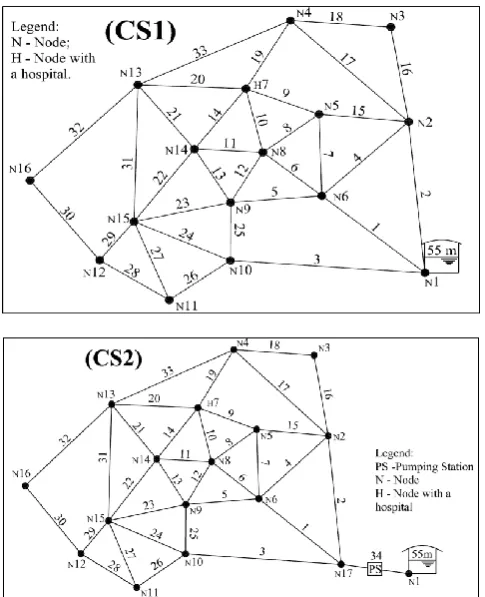
Figure 1. Network schemes: case study 1 (CS1) and case study 2 (CS2). 3

4

5

6

7

8

9

10

11

12

Figure 1.Network schemes: case study 1 (CS1) and case study 2 (CS2).

Fig. 1, the network is gravity fed by a single reservoir with a fixed level of 55 m and comprises 33 pipes and 16 nodes. Case study 2 (CS2), Fig. 1, is similar but it introduces a PS downstream of the reservoir (link 34). This PS is a contin-gency structure that should be used only in abnormal work-ing conditions. As these situations are usually short-lived, the energy consumption and its cost were neglected.

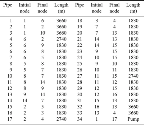
The characteristics of the pipes are given in Table 1 and the nodes in Table 2. The commercial diameters (and their cost) used in the present study are given in Table 3. The head losses were calculated using the Hazen-Williams equation. It is also assumed that there is a hospital in node 7 with special pressure and demand requirements.

A multiple scenario approach was used to design the net-work for the two case studies:

Table 1.Characteristics of the pipes.

Pipe Initial Final Length Pipe Initial Final Length node node (m) node node (m)

1 1 6 3660 18 3 4 1830

2 1 2 3660 19 7 4 1830

3 1 10 3660 20 7 13 1830

4 6 2 2740 21 14 13 1830

5 6 9 1830 22 14 15 1830

6 6 8 1830 23 9 15 1830

7 6 5 1830 24 10 15 1830

8 5 8 1830 25 9 10 1830

9 5 7 1830 26 10 11 1830

10 8 7 1830 27 11 15 2740

11 8 14 1830 28 11 12 1830

12 8 9 1830 29 12 15 1830

13 9 14 1830 30 12 16 1830 14 14 7 1830 31 15 13 1830

15 2 5 1830 32 16 13 3660

16 2 3 1830 33 13 4 3660

17 2 4 2740 34 1 17 Pump

– Scenario 6: IPD and a fire in node 12 (200 l s−1);

– Scenario 7: IPD and a fire in node 13 (200 l s−1_).

The IPD is 1.8 times the average discharge. For case study 2, the maximum nodal pressures should not exceed 60 m for scenario 1 and should not exceed 90 m for scenarios 2 to 7, for the nodes of the network (N2 to N16). In the pipe break scenarios (2 to 4), it is assumed that the pipe that breaks can be isolated without compromising the supply of the respec-tive end nodes. For scenario 1, the minimum desired and ad-missible pressures are 30 m for all nodes; for scenarios 2 to 7 the minimum desired pressure is 25 m and the minimum ad-missible pressure is 10 m for all nodes except node 7; as node 7 supplies a hospital, for scenarios 2 to 7 the minimum de-sired pressure is 30 m and the minimum admissible pressure is 25 m. In scenarios 5 to 7 it is assumed that the firefighting demands are completely satisfied even if the fire node pres-sure is lower than the desired prespres-sure.

4 Results and comparisons

This work proposes a different approach to toughening a WSS so that it can cope with normal and abnormal situa-tions and then compares it with another possible solution. In both case studies the network must work under 7 different operating scenarios (the traditional peak design flow and 6 extreme scenarios – 3 burst pipe scenarios and 3 firefighting scenarios). The objective function of the robust optimization model includes pipe costs, pumping station costs (construc-tion and equipment) and penalties for pressure and demand violations. Network robustness can only be achieved in case study 1 by increments in pipe diameters. The flow must have alternative paths with enough capacity to carry bigger dis-charges to overcome the extreme scenarios. Network

robust-Table 2.Characteristics of the nodes.

Node Ground Peak Node Ground Peak Elevation Discharge Elevation Discharge

(m) (l s−1_{) (m) (l s}−1₎

1 0 0 10 0 43.889

2 0 43.889 11 0 43.889

3 0 43.889 12 0 43.889

4 0 43.889 13 0 43.889

5 0 43.889 14 0 43.889

6 0 43.889 15 0 43.889

7 0 43.889 16 0 43.889

8 0 43.889 17 0 0

9 0 43.889

ness can also be achieved in case study 2 by using the pump-ing station to increase the head at the reservoir. For the ex-treme scenarios, which occur occasionally and only for short periods of time, it was assumed that the maximum nodal pressure should not exceed 90 m (this constraint limits the pumping head and avoids potentially excessive pressure in the network). This approach avoids the large pipe diameter increase imposed by the case study 1 conditions (gravity fed network).

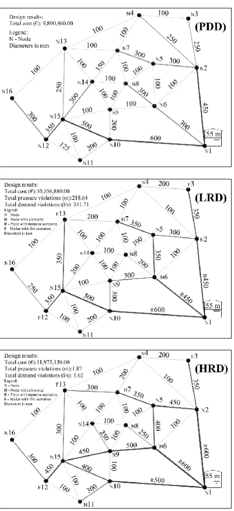
The decision variables of the robust optimization model are: case study 1 – pipe diameters; case study 2 – pipe di-ameters and pumping head for scenarios (2 to 7) of fixed velocity pumps. The peak discharge design (PDD) is deter-mined by solving the model considering only scenario 1. This design is used to compare the cost differences that the ro-bustness solutions imply. To synthesize the results, only the PDD solution, the low robustness design (LRD) and the high robustness design (HRD) for each of the two case studies are presented. However, intermediate robust solutions can be achieved by considering different levels of robustness for the network (Cunha and Sousa, 2009). The LRD assumes a low probability of the extreme scenarios occurring and includes small penalty coefficients. The HRD is obtained assuming a high probability that the extreme scenarios will occur and large penalty coefficients. Figures 2 and 3 show the details of the solutions found for case studies 1 and 2. These fig-ures show the commercial diameter chosen for each pipe in millimetres, the PS head in meters for the different scenarios considered, the partial and total cost of the solutions and also the total pressure and demand violations.

The “Total pressure violations” given in Figs. 2 and 3 rep-resent the sum of all the pressure violations at all the network nodes and for all the scenarios. A similar procedure was used to compute the “Total demand violations”.

Table 3.Commercial diameters, unit costs and Hazen-Williams coefficients.

Diameters Unit cost H-W Diameters Unit cost H-W

(mm) (€/m) Coefficients (mm) (€/m) Coefficients

100 87 120 450 247 120

125 97 120 500 277 120

150 102 120 600 371 120

200 120 120 700 465 120

250 147 120 800 559 120

300 157 120 900 653 120

350 187 120 1000 747 120

400 215 120

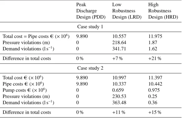
Table 4.Total cost differences for the two case studies.

Peak Low High

Discharge Robustness Robustness

Design (PDD) Design (LRD) Design (HRD)

Case study 1

Total cost=Pipe costs€(×106_{) 9.890 10.557 11.975}

Pressure violations (m) 0 218.64 1.87

Demand violations (l s−1_{) 0 341.71 1.62}

Difference in total costs 0 % +7 % +21 %

Case study 2

Total cost€(×106_{) 9.890 10.997 11.397}

Pipe costs€(×106_{) 9.890 10.337 10.442}

Pump costs€(×106_{) 0 0.659 0.975}

Pressure violations (m) 0 230.53 0.25

Demand violations (l s−1_{) 0 363.48 0.36}

Difference in total costs 0 % +11 % +15 %

scenarios considered. It should also be pointed out that those “main rings” always embrace the critical node – Hospital (H7). As expected, the case study 1 solutions use larger pipe diameters than case study 2. In fact, the PS plays an impor-tant role in ensuring the network supply for case study 2, instead of using larger pipe diameters; reliability is achieved by the PS increasing the head at the reservoir for the extreme scenarios.

Table 4 shows a comparison of the solutions obtained for the case studies (cost, pressure violations and demand vio-lations, for the designs presented in Figs. 2 and 3). The in-creases in total costs for the LRD and the HRD are calculated taking the PDD cost as reference. The penalty coefficients for the two case studies were fixed so as to obtain solutions with similar pressure and demand violations for both case studies. Some conclusions can be drawn from Table 4. In case study 1, the LRD costs are 7 % higher, but to get an HRD would require spending 21 % more than the cost of the tra-ditional PDD solution. As robustness is achieved solely by enlarging the pipe diameters, the HRD for case study 1 has

the highest total cost for the pipes – 11.975×106€(this is the design with largest pipe diameters). In terms of network behaviour, this design is sufficiently reliable to perform well even in the extreme scenarios. However, for normal working conditions the pipes are overdesigned, which means low ve-locities and high residence times, conditions that may lower water quality and safety. The option to raise the reliability of a WSS to high levels only by increasing the pipe diameters should therefore be avoided if there are other alternatives that can be implemented.

The LRD for case study 2 is more costly than that for case study 1. These case studies show that, in terms of cost, for low robustness designs it is preferable to enlarge the pipes instead of using a PS. For less reliable solutions, a minor in-crease of pipe diameters is required for the network which will be cheaper than implanting a pumping station down-stream of the reservoir, even for low pumping heads.

18 1

2

3

Figure 2. Designs for case study 1: (PDD) peak discharge (LRD) low robustness and (HRD) 4

high robustness. 5

6

Figure 2.Designs for case study 1: (PDD) peak discharge (LRD) low robustness and (HRD) high robustness.

with the extreme scenarios. The combination of these ele-ments resulted in a high robustness design for a lower cost in-crease than case study 1. Furthermore, this approach reduces the overdesign problems. By introducing additional power at the reservoir, the PS avoids enlarge pipes to ensure the min-imum desired pressures at the network nodes. In conclusion, these case studies indicate that for high robustness designs it

19 1

2

Figure 3. Designs for case study 2: (LRD) low robustness and (HRD) high robustness. 3

4

Figure 3. Designs for case study 2: (LRD) low robustness and (HRD) high robustness.

is preferable to use a PS combined with smaller enlarging of the pipes than to rely on more general of the pipes.

5 Conclusions

To obtain high robustness solutions WSSs must be designed to cope with extreme operating conditions during their life cycle. The uncertainty related to future operating conditions should be taken into account early in the design stage. This work has presented a robust optimization model to help deci-sion makers attain a good trade-offbetween reliability and cost. The performance of this method was illustrated by means of two case studies. The reliability of the water supply systems was ensured by two different strategies: 1st – design-ing the system to cope with the extreme operatdesign-ing conditions by increasing the pipe diameters; 2nd – designing the system for normal operating conditions and introducing a pumping station to deal with the extreme operating conditions.

high water residence times. The 2nd strategy, which is in-novation proposed in this work, can also be viewed as an alternative for existing WSSs. For some existing systems, strengthening the infrastructure links may be difficult if it involves construction works in urban areas and it could also be prohibitively expensive, so innovative strategies should be used. For future developments of this work, consideration of the water age can be added to the determination of solutions. The water quality could be used to evaluate the design al-ternatives so that the solution can be further optimized for a truly robust design. It could also be important to under-stand the influence of the maintenance costs of many pump-ing stations required as contpump-ingence infrastructures in large systems, which is likely the case in real water systems. A life cycle cost analysis of the strategies (including the main-tenance of pipes and pumps) can be conducted to choose the design of a robust solution.

Acknowledgements. This work has been financed by FEDER funds through the Programa Operacional Factores de Competitivi-dade – COMPETE, and by national funds from FCT – Fundac¸˜ao

para a Ciˆencia e Tecnologia under grant PTDC/ECM/64821/2006.

The participation of the first author in the study is supported by FCT – Fundac¸˜ao para a Ciˆencia e Tecnologia through Grant

SFRH/BD/47602/2008.

Edited by: R. Farmani

References

Aarts, E. and Korst, J.: Simulated Annealing and Boltzmann Ma-chines: A Stochastic Approach to Combinatorial Optimization and Neural Computing, Chichester, England, John Wiley & Sons, 1989.

Babayan, A. V., Savic, D. A., Walters, G. A., and Kapelan, Z. S.: Robust Least-Cost Design of Water Distribution Networks Using Redundancy and Integration-Based Methodologies, J. Water Res. Pl.-ASCE, 133, 67–77, 2007.

Carr, R. D., Greenberg, H. J., Hart, W. E., Konjevod, G., Lauer, E., Lin, H., Morrison, T., and Phillips, C. A.: Robust optimization of contaminant sensor placement for community water systems, Math. Program., 107, 337–356, 2006.

Cunha, M. C. and Sousa, J.: Water Distribution Network Design Optimization: Simulated Annealing Approach, J. Water Res. Pl.-ASCE, 125, 215–221, 1999.

Cunha, M. C. and Sousa, J.: Hydraulic Infrastructures Design Using Simulated Annealing, J. Infrastruct. Syst., 7, 32–39, 2001. Cunha, M. C. and Sousa, J.: Robust design of water distribution

networks: a comparison of two different approaches, in: Proc.

CCWI, Sheffield, UK, CRC Press, 181–187, 2009.

Cunha, M. C. and Sousa, J. J. O.: Robust Design of Water Distribu-tion Networks for a Proactive Risk Management, J. Water Res. Pl.-ASCE, 136, 227–236, 2010.

DIEDE and AIDIS: Integrated risk management to protect drinking water and sanitation services facing natural disasters, IRC Inter-national Water and Sanitation Centre, The Netherlands, thematic overview paper no 21, 54 pp., 2008.

Giustolisi, O., Laucelli, D., and Colombo, A. F.: Deterministic ver-sus Stochastic Design of Water Distribution Networks, J. Water Res. Pl.-ASCE, 135, 117–127, 2009.

Jeong, H. S., Qiao, J., Abraham, D. M., Lawley, M., Richard, J., and Yih, Y.: Minimizing the Consequences of Intentional Attack on Water Infrastructure, Comput.-Aided Civ. Inf., 21, 79–92, 2006. Mulvey, J., Vanderbei, R., and Zenios, S.: Robust Optimization of

Large-Scale Systems, Oper. Res., 43, 264–281, 1995.