Nonlinear cochlear signal processing

(1)

Nonlinear Cochlear Signal Processing

Jont B. Allen

Florham Park, NJ

March 13, 2001

Introduction

This chapter describes the mechanical function of the cochlea, or inner ear, the organ that converts signals from acoustical to neural. Many cochlear hearing disorders are still not well understood. If systematic progress is to be made in improved diagnostics and treatment of these disorders, a clear understanding of basic principles is essential. Models of the cochlea are useful because they succinctly describe auditory perception principles.

The literature is full of speculations about various aspects of cochlear function and dysfunction. Unfortunately, we still do not have all the facts about many important issues. One of the most important examples of this is how the cochlea attains its sensitivity and frequency selectivity, which is very much a matter of opinion. A second important example is dynamic range (acoustic intensity) compression, due to the operation of cochlear outer hair cells (OHC).

However today our experimental knowledge is growing at an accelerating pace because of a much tighter focus on the issues. We now know that the answers to the questions of cochlear sensitivity, selectivity, and dynamic range, lie in the function of the outer hair cells. As a result, a great deal of attention is now being concentrated on outer hair cell biophysics. This effort is paying off at the highest level. Three examples come to mind. First is multiband compression hearing aids. This type of signal processing, first proposed in 1938 by Steinberg and Gardner, has revolutionized the hearing aid industry in the last 10 years. With the introduction of compression signal processing, hearing aids work. This powerful circuit is not the only reason hearing aids of today are better. Better electronics and trans-ducers have made impressive strides as well. In the last few years the digital barrier has finally been broken. One might call this the last frontier in hearing aid development.

A second example is the development of otoacoustic emissions (OAE) as a hearing diagnostic tool. Pioneered by David Kemp and Duck Kim, and then by many others, this tool allows for the cochlear evaluation of infants only a few days old. The identification of cochlear hearing loss at such an early stage is dramatically changing the lives of these children and their parents for the better. While it is tragic to be born deaf, it is much more tragic to not recognize the deafness until the child is 3 year old, when he or she fails to learn to talk. With proper and early intervention, these kids lead normal, productive lives.

A third example continues to evade us, namely how the auditory system, including the cochlea and the auditory cortex, processes human speech. If we can solve this grail-like problem, we will fundamentally change the way humans and computers interact, for the better. The ultimate hearing aid is the hearing aid with built in robust speech recognition. We have no idea when this will come to be, and it is undoubtedly many years off, but when it happens it will be a revolution that will not go unnoticed.

Chapter Outline: Several topics will be reviewed. First, the history of cochlear models, including extensions that have taken place in recent years. These models include both macromechanics and micromechanics of the tectorial membrane and hair cells. This leads to comparisons of the basilar membrane, hair cell, and neural frequency tuning. The role of nonlinear mechanics and dynamic range are covered to help the student understand the importance of modern wideband dynamic range compression hearing aids. Hearing loss, loudness recruitment, as well as other important topics of modern hearing health care, are briefly discussed.

(3)

knowledge about cochlear anatomy or function, many good text books exist that can fulfill that need better than this more advanced review paper [1, 2].

Figure 1: Cross section through the cochlear duct showing all the major structures of the cochlea. The three chambers are filled with fluid. Reissner’s membrane is an electrical barrier and is not believed to play a mechanical role.

Function of the Inner Ear

(4)

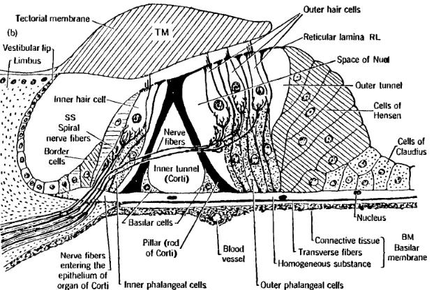
Figure 2: This cross section of the Organ of Corti shows the inner and outer hair cells, pillar cells and other supporting structures, the basilar membrane (BM), and the tectorial membrane (TM).

Inner Hair Cells. In very general terms, the role of the cochlea is to convert sound at the eardrum into neural pulse patterns along 30,000 neurons of the human auditory (VIII

) nerve. After being filtered by the cochlea, a low level pure tone has a narrow spread of excitation which excites the cilia of about 40 contiguous inner hair cells. Cilia excitation is a narrow band signal with a center frequency that depends on the inner hair cell’s location along the basilar membrane. Each hair cell is about 10 micrometers in diameter while the human basilar membrane is about 35 mm in length (35,000 microns). Thus the neurons of the auditory nerve encode the responses of about 3,500 inner hair cells which form a single row of cells along the length of the BM. Each inner hair cell voltage is a lowpass filtered representation of the detected inner hair cell cilia displacement [5]. Each hair cell is connected to many neurons. In the cat, for example,1_{approximately 15–20 neurons encode}

each of these narrow band inner hair cells with a neural timing code. It is widely believed that the neuron information channel between the hair cell and the cochlear nucleus is a combination of the mean firing rate and the relative timing between neural pulses (spikes). The mean firing rate is reflected in the loudness coding, while the relative timing carries more subtle cues, including for example pitch information and speech voicing distinctions.

Outer Hair Cells. As shown in Fig. 2 there are typically 3 (sometimes 4) outer hair cells (OHCs) for each inner hair cell (IHCs), leading to about 12,000 for the human cochlea. Outer hair cells are used for intensity dynamic range control. This is a form of nonlinear signal processing, not dissimilar to Dolby sound processing.2 It is well known (as was first proposed by Lorente de No [7] and Steinberg and Gardner [8]) that noise damage of

1_{It is commonly accepted that all mammalian cochleae are similar in function. The frequency range of operation} differs between species.

(5)

“nerve cells” (i.e., OHCs) leads to a reduction of dynamic range, a disorder clinically called

dynamic range recruitment.

We may describe cochlear processing two ways. First in terms of the signal represen-tation at various points in the system. Second, in terms of models. These models are our most succinct means of conveying the results of years of detailed and difficult experimental work on cochlear function. The body of experimental knowledge has been very efficiently represented (to the extent that it is understood) in the form of these mathematical models. When no model exists (e.g., because we do not understand the function), a more basic description via the experimental data is necessary. Several good books and review papers are available which make excellent supplemental reading [9, 1, 10, 11, 4, 12].

For pedagogical purposes the discussion is divided into five sections: Section 1

Macrome-chanics describes the fluid motions of the scalae and treats the basilar membrane as a

dynamical system having mass, stiffness, and damping. Section 2 Inadequacies of the 1

model describes the experimental data that characterizes the nonlinear cochlea. Section

3 OHC Transduction, describes the electromechanical action of the outer hair cell on the basilar membrane. Most important is the nonlinear feedback provided by the outer hair cell, leading to the dynamic range compression of the inner hair cell excitation. Section 4

Mi-cromechanics describes the models of the motion of the Organ of Corti, the inner and outer

hair cell cilia, the tectorial membrane, and the motion of the fluid in the space between the reticular lamina and the tectorial membrane. Much of this section has been adapted from an earlier article [13]. Finally in Sec. 5 we briefly summarize the entire paper.

A warning to the reader: Due to experimental uncertainty there is diverse opinion in the literature about certain critical issues. While there are many areas of agreement, this paper is directed on those more interesting controversial topics. For example, (a) it is very difficult to experimentally observe the motion of the basilar membrane in a fully functional cochlea; (b) questions regarding the relative motion of the tectorial membrane to other adjacent structures are largely a matter of conjecture. Some of these questions are best investigated theoretically. The experimental situation is improving as new techniques are being invented. As a result, a multitude of opinions exist as to the detailed function of the various structures.

On the other hand, firm and widely accepted indirect evidence exists on how these structures work. This indirect evidence takes on many forms, such as neuro- and psy-chophysical, morphological, electrochemical, mechanical, acoustical, and biophysical. All these diverse forms of “indirect” data may be related via models. Their value is not depre-ciated because of their indirect nature. In the end, all the verifiable data must, and will, coexist.

1 Macromechanics

Typically the cochlea is treated as an uncoiled long thin box, as shown in Fig. 3. This represents the starting point for the macromechanical models.

(6)

Helicotrema

RW Stapes/OW

Scala Tympani

Scala Vestibuli Tectorial Membrane

Basilar Membrane

BASE

x = 0 x = L

APEX

Figure 3: Box model of the cochlea. The Base ( =0) is the high frequency end of the cochlea while the Apex ( =

) carries the low frequencies.

1.1 The early history of cochlear modeling.

I am told that Helmholtz’s widely recognized model of the cochlea was first presented by him in Bonn in 1857 (subsequently published in a book on his public lectures in 1857 [14]), and again later in 1863 in chapter VI and in an appendix of On the Sensations of Tone [15]. Helmholtz likened the cochlea to a bank of highly tuned resonators, which are selective to different frequencies, much like a piano or a harp [14, page 22-58], with each string representing a different place on the basilar membrane. The model he proposed is not very satisfying however, since it left out many important features, the most important of which includes the cochlear fluid which couples the mechanical resonators together. But given the publication date, it is an impressive contribution by this early great master of physics and psychophysics.

The next major contribution, by Wegel and Lane (1924), stands in a class of its own even today, as a double barreled paper having both deep psychophysical and modeling insight.3 _{The paper was the first to quantitatively describe the details of how a high level}

low frequency tone effects the audibility of a second low level higher frequency tone (i.e., the upward spread of masking). It was also the first publication to propose a “modern” model of the cochlea. If Wegel and Lane had been able to solve their model equations (of course they had no computer to do this), they would have predicted cochlear traveling waves. It was their mistake, in my opinion, to make this one paper. The modeling portion of their paper has been totally overshadowed by their experimental results.

I know of only two other early major works in cochlear modeling, one by Fletcher [17], and several by Ranke starting in 1931 (for a historical review see [18, 19]).

Contrary to some opinion [20], the significance of cochlear viscous fluid damping (a measure of the energy loss) was shown by B ´ek ´esy to be very small [21, 22]. Fletcher’s 1951 model [21] (Eq. 8) was the first to quantitatively consider fluid viscosity. In fact the inner ear is nearly a lossless system.4 The significance of this is great. Imagine a nearly lossless bouncing ball. Such a ball would bounce wildly, similar to a “super ball.” Low-loss structures, such as the cochlea, have unusual properties that appear to defy the laws of physics.

It was the experimental observations of G. von B ´ek ´esy starting in 1928 on human ca-daver cochleae which unveiled the physical nature of the basilar membrane traveling wave.

3_{Fletcher published much of the Wegel and Lane data one year earlier [16]. It is not clear to me why Wegel and} Lane are always quoted for these results rather than Fletcher. In Fletcher’s 1930 modeling paper, he mentioned that he was the subject in the Wegel and Lane study. It seems to me that Fletcher deserves some of the credit.

(7)

What von B ´ek ´esy found (consistent with the 1924 Wegel and Lane model) was that the cochlea is analogous to a “dispersive” transmission line where the different frequency com-ponents which make up the input signal travel at different speeds along the basilar mem-brane, thereby isolating each frequency component at a different place along the basilar membrane. He properly named this dispersive wave a “traveling wave.” He observed the traveling wave using stroboscopic light, in dead human cochleae, at sound levels well above the pain threshold, namely above 140 dB SPL.5 _{These high sound pressure levels were}

required to obtain displacement levels that were observable under his microscope. von B ´ek ´esy’s pioneering experiments were considered so important that in 1961 he received the Nobel prize.

Over the intervening years these experiments have been greatly improved, but von B ék ésy’s fundamental observation of the traveling wave still stand. His original experi-mental results, however, are not characteristic of the responses seen in more recent ex-periments, in many important ways. These differences are believed to be due to the fact that B ék ésy’s cochleae were dead, and because of the high sound levels his experiments required.

Today we find that the traveling wave has a more sharply defined location on the basi-lar membrane for a pure tone input than observed by von B ´ek ´esy. In fact, according to measurements made over the last 20 years, the response of the basilar membrane to a pure tone can change in amplitude by more than five orders of magnitude per millimeter of distance along the basilar membrane (i.e., 300 dB/oct is equivalent to 100 dB/mm in the cat cochlea).

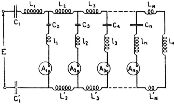
Figure 4: Figure 7b from 1924 Wegel and Lane paper.

To describe this response it is helpful to call upon the 1924 Wegel and Lane and the 1930 Fletcher model of macromechanics, the transmission line model, which was first quantitatively analyzed by J. J. Zwislocki (1948, 1950), Peterson and Bogart (1950), and Fletcher (1951). The transmission line model is also called the one-dimensional (1 ), or

long-wave model.

(8)

V

p

P₂

1

P

V₁ V₂

Zp iω

iω iω

iω

-+ ₊

-(volume velocity)

(pressure)

R

Mp p

ρ

A 2 s Z /2 =

s

ρ

2 As

K (x)_p (x) (x)

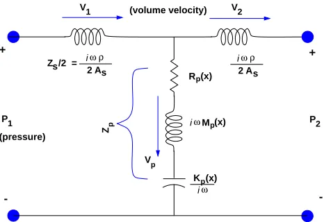
Figure 5: A single section of the electrical network 1 model described by Wegel and Lane. The model is built from a cascade of such section.

1.2 The 1

model of the cochlea

Zwislocki (1948) was first to quantitatively analyze Wegel and Lane’s macromechanical cochlear model, explaining B ´ek ´esy’s traveling wave. Wegel and Lane’s 1924 model is shown in Figs. 4 and 5. The stapes input pressure is at the left, with the input velocity

, as shown by the arrow, corresponding to the stapes velocity. This model represents

the mass of the fluids of the cochlea as electrical inductors and the BM stiffness as a capacitor.Electrical circuit networks are useful when describing mechanical systems. This is possible because of an electrical to mechanical analog that relates the two systems of equations, and because the electrical circuit elements comprise a de facto standard for describing such equations. It is possible to write down the equations that describe the system from the circuit of Fig. 5, by those trained in the art. Engineers and scientists frequently find it easier to “read” and think in terms of these pictorial circuit diagrams, than to interpret the corresponding equations.

1.2.1 Impedance.

During the following discussion it is necessary to introduce the concept of a 1-port (two-wire) impedance. Impedance is typically defined in the frequency domain in terms of pure tones , which is characterized by amplitude , driving frequency , and

phase . Ohm’s Law defines impedance as

Impedance

effort flow

(1)

In an electrical system the impedance is the ratio of a voltage (effort) over a current (flow). In a mechanical system it is the force (effort) over the velocity (flow). I next give three important examples:

Example 1: The impedance of the tympanic membrane (TM, or eardrum) is defined in

(9)

referred to here are conventionally described using complex numbers, to account for the phase relationship between the two.

Example 2: The impedance of a spring is given by

(2)

where

is the stiffness of the spring and is the frequency. This element is represented as

two straight lines (Fig. 5) close together, which looks like two physical plates. The important term

(3) in the denominator, indicates that the impedance of a spring has a phase of

(-90 ).

This phase means that when the velocity is , the force is . The definition

of Eq. 2 follows from Hooke’s Law which says that the force and displacement of a

spring are proportional, namely

(4) Since the velocity

, and the definition of the impedance is ratio of

, Eq. 2 follows.

Example 3: From Newton’s Law where is the force, is the mass, and

acceleration

. The electrical element corresponding to a mass is an “inductor,” indicated in Fig. 5 by a coil. Thus for a mass

(5)

From Eq.’s 2 and 5, the magnitude of the impedance of a spring decreases as

, while

the impedance magnitude of a mass is proportional to . The stiffness with its -90 phase

is called a lagging phase, while the mass with its +90 phase is called a leading phase.

1.2.2 Th ´evenin equivalence

When dealing with impedance circuits there is a very important concept called the Th ´evenin

equivalent circuit. In 1883 a French telegraph engineer L ´eon Th ´evenin showed6that any active 1-port circuit, of any complexity, is equivalent to a series combination of a source

voltage

and a source impedance

. These two elements are uniquely defined by performing two independent measurements. Any two independent measurements would do, but for the purpose of definition, two special measurements are best. The first defines

, which is called the open circuit voltage. This is the voltage measured with no load on the system. The second measurement is the short circuit (unloaded ) current

, defined as the current when the two terminals are connected together. By taking the ratio of the open circuit voltage and the short circuit current, the Th ´evenin impedance is obtained

. The classical example is a battery. The open circuit voltage defines the Th ´evenin volt-age

, which is the voltage measured with no load. The short circuit current

is the cur-rent measured with a wire across the terminals (don’t try this!). The Th ´evenin impedance

is the unloaded voltage divided by the short circuit current.

As a second example consider an earphone. When unloaded, by placing the earphone in a very small cavity so that it has very little air to move, it can produce an “open circuit” pressure. However, when loaded by placing it in the ear canal, the earphone pressure is

(10)

reduced, due to the load of the ear canal. If it were placed in water, the load would be very large, and the corresponding pressure would be small. In this case the “short circuit current” corresponds to volume velocity of water that the diaphragm of the earphone can move. The Th ´evenin parameters are the pressure measured in the small cavity, and the impedance defined by the Th ´evenin pressure divided by the volume velocity measured when place in in the water load.

The Th ´evenin parameters are needed to characterize a hair cell’s properties.

1.3 2-port analysis

The concept of a 1-port impedance and of a Th ´evenin equivalence circuit has been gen-eralized by defining a 2-port (4-wire connection) [30]. This is a very important modeling tool that is used every time we must deal with both an input and an output signal. This methodology is called 2-port analysis by engineers [31, 30, 32], referring to the fact that a transducer has an input and output. A related literature is called Bond Graph analysis [33]. A pair of “impedance” (conjugate) variables effort and flow (see section Sec. 1.2.1 and [31]), are used in each of two domains, the input and the output, to characterize the transducer.

The 2-port relation properly characterizes the relations between an input effort and flow, which we denote as lower case variables

, and an output effort and flow, characterized

by upper case variables

. This characterization is in the frequency domain, and it

re-quires four functions of complex frequency

frequency, which are traditionally called

[30]. These four functions completely characterize the linear 2-port.

Complex frequency is the necessary frequency variable for functions that are causal (one

sided in time), as in the case of impedances.

(6)

In later sections we shall see that all of the impedance and Th ´evenin properties are cap-tured in this one matrix equation. A 2-port is called reciprocal if it is reversible. For recipro-cal systems, (7) If a system is reciprocal then it is bidirectional because when the determinant of the

matrix is 1 (Eq. 7), the inverse system must exist.

Each section of the the Wegel and Lane model Fig. 5. has a series impedance

and a shunt impedance

. Thus it is a cascade of three

matrices, which may be written

as (8)

This provides a mathematical formulation of a section of the Wegel and Lane model. The details for doing this are derived in Pipes [30].

If the system is reversed and its topology is identical then,

. This is called a

symmetric network, which is a common special case of a reciprocal 2-port. For example,

(11)

Reciprocal systems. The classic example of a reciprocal network is a piezoelectric crys-tal, while the classic example of a non reciprocal network is a transistor. More to the point, outer hair cell forward transduction, which characterizes the relation between the cell’s cilia displacement (the input) and the cell’s membrane voltage (the output), is typically charac-terized as non-reciprocal. Reverse transduction, which characterizes the membrane volt-age (the input) and the output motility (the output) is believed (but not yet proven) to be reciprocal.

1.3.1 Anatomy of the model.

Different points along the basilar membrane are represented by the cascaded sections of the transmission line model of Fig. 5. The position along the model corresponds to the lon-gitudinal position along the cochlea. The series (horizontal) inductors (coils) represent the fluid mass (inertia) along the length of the cochlea, while the elements connected to ground (the common point along the bottom of the figure) represent the mechanical (acoustical) impedance of an element of the corresponding section of the basilar membrane. In the Wegel and Lane model the partition impedance, defined as the pressure drop across the basilar membrane divided by its volume velocity per unit length, has the form

(9)

where

is the resistance. Each inductor going to ground represents the partition and fluid mass per unit length

of the section, while the capacitor represents the compliance

[the reciprocal of the stiffness

] of the section of basilar membrane. Note that and

are impedances, but is simply a mass, and

a stiffness, but not an impedance. The stiffness decreases exponentially along the length of the cochlea, while the mass is frequently approximated as being independent of position. The position variable is frequently called the place variable.

Driving the model To understand the inner workings of Wegel and Lane’s circuit Fig. 5, assume that we excite the line at the stapes with a sinusoidal velocity of frequency . Due

to conservation of fluid mass within the cochlea (fluid mass cannot be created or destroyed in this circuit), at every instant of time the total volume through the basilar membrane must equal the volume displaced by the stapes. Simultaneously, the round window membrane, connected to the scala tympani, must bulge out by an equal amount [34]. In practice the motion of the basilar membrane is complicated. However the total volume displacement of the basilar membrane, at any instant of time, must be equal to the volume displacement of the stapes, and of the round window membrane.

Flow in the model. Consider next where the fluid current

will flow, or where it can flow.

(12)

f=8 kHz

|Z| (dB)

_{M 2 f}

X

_cf(8)

X

_cf(1)

BASE

K(x)/2 f

π

f=1 kHz

BM IMPEDANCE

LOG-MAGNITUDE

X

APEX

PLACE

Figure 6: Plot of the log-magnitude of the impedance as a function of place for two different frequencies of 1 and 8 kHz. The region labeled is the region dominated by the stiffness and

has impedance . The region labeled is dominated by the mass and has impedance .

The characteristic places for 1 and 8 kHz are shown as

cf.

the only impedance element that contributes to the impedance is the resistance. This point is called the resonant point, which is defined as that frequency cf where the mass and

stiffness impedance are equal

cf

(10)

Solving for cf defines the cochlear map function, which is one of the most important

concepts of cochlear modeling

cf

(11)

The inverse of this function cf specifies the location of the “hole” shown in Fig. 6 as a

function of frequency.

Basal to the resonant point cf of Fig. 6, the basilar membrane is increasingly stiff

(has a large capacitive impedance), and apically (to the right of the resonant point), the impedance is a large mass reactance (inductive impedance). In this apical region the impedance is largely irrelevant since little fluid will flow past the mechanical hole labeled

cf at the minimum. The above description is dependent on the input frequency since

the location of the hole (the impedance minimum) is frequency-dependent.

This description is helpful in our understanding in why the various frequency compo-nents of a signal are splayed out along the basilar membrane. If we were to put a pulse of current in at the stapes, the highest frequencies that make up the pulse would be shunted close to the stapes, while the lower frequencies would continue down the line. As the pulse travels down the basilar membrane, the higher frequencies are progressively removed, un-til almost nothing is left when the pulse reaches the right end of the model (the helicotrema end, the apex of the cochlea).

Let’s next try a different mental experiment with this model. Suppose that the input at the stapes were a slowly swept tone or chirp. What would the response at a fixed point on the basilar membrane look like at one point along the basilar membrane? The ratio of the displacement BM to stapes displacement, as a function of frequency , has a shallow

(13)

Derivation of the cochlear map function. The cochlear map function cf plays a very

important role in cochlear mechanics, has a long history, and is known by many names [17, 35, 36, 37, 38, 39]. The following derivation for the form of the cochlear map, based on “counting” critical bands, is from Fletcher [40] and Greenwood [39]. The number of critical

bands may be found by integrating the density of critical bandwidth over frequency

in Hz and over place in mm. The cochlear map function

cf is then found

by equating these two integrals.

The critical bandwidth is the effective width in frequency of the spread of energy

on the basilar membrane. It has been estimated by many methods. The historical methods used by Fletcher were based on the critical ratio and the pure tone just noticeable

difference in frequency (JND ). These two psychoacoustic measures have a constant ratio

of 20 between them [36] and page 171 of [41], namely the critical bandwidth in Hz equals 20 JND in Hz. From [17] (Eq. 6)

JND

(12)

with in mm. Thus the critical ratio (in dB)

is of the form where and are

constants. The critical bandwidth, converted back to Hz, is

!#"

(13)

This was verified by Greenwood [39], page 1350, Eq. 1.

The critical spread is the effective width of the spread of energy on the basilar

membrane due to a pure tone. Based on an argument of Fletcher’s, Allen found that in the cat corresponds to about 2.75 times the width of the basilar membrane$%'& [40],

namely

(*)

$+'&

(14) The two ratio measures , *- and , ./ define the density of critical bands

in frequency and place, and each may be integrated to find the number of critical bands

. Equating these two functions results in the cochlear map function cf

10

,

02 cf

,

(15)

For a discussion of work after 1960 on the critical band see [40, 12].

Cochlear map in the Cat In 1982 Liberman [42] and in 1984 Liberman and Dodds [43] directly measured cf in the cat and found the following empirical formula

cf 43

)

65

87

9:

(16)

(14)

f(f)

(x)_x

Place (cm)

Log(CF) (kHz)

L 0

CAT COCHLEAR MAP

Slope = 3 mm/octave

∆

F_max

Figure 7: Cochlear map of the cat following Liberman and Dodds, Eq. 16. This figure also shows how a critical band and a critical spread area related through the cochlear map function.

2 Inadequacies of the 1

,

model (Summary of

experimen-tal data)

Wegel and Lane’s transmission line model was a most important development, since it was a qualitative predictor (by 26 years) of the experimental results of von B ´ek ´esy, and it was based on a simple set of physical principles (conservation of fluid mass, and spatially variable basilar membrane stiffness). The Wegel and Lane 1 model was the theory of choice until the 1970’s when:

numerical model results became available, which showed that 2 and 3 models were more frequency selective than the 1 model,

experimental basilar membrane observations showed that the basilar membrane mo-tion had a nonlinear compressive response growth, and

improved experimental basilar membrane observations became available which showed increased nonlinear cochlear frequency selectivity.

In the next section we review these developments.

2.1 Contemporary history of cochlear modeling

In 1976 George Zweig and colleagues pointed out that an approximate but accurate solu-tion for the 1 model could be obtained using a well known method in physics called the “WKB” approximation [44]. The method was subsequently widely adopted [45]. The results of Zweig et al. were similar to Rhode’s contemporary basilar membrane data [46], but very different than contemporary neural tuning curve responses [47].7

(15)

The discrepancy in frequency selectivity between basilar membrane and neural re-sponses has always been, and still is, the most serious problem for the cochlear modeling community. In my view, this discrepancy is one of the most basic unsolved problems of

cochlear modeling. Progress on this front has been seriously confounded by the

uncer-tainty in, and the interpretation of, the experimental data. We shall soon return to this same point.

2 models: The need for a two-dimensional (2 ) theory was first explicitly presented by Ranke [18]. In the 70’s several 2 model solutions8 _{became available [48, 49, 50, 51, 52].}

These results made it clear that the 1 theory, while a useful approximation, must be used only with cautioned thoughtful care.

Soon it was possible to compute the response of a 2 , and even the response of a 3 geometry [53, 45, 54]. As the complexity of the geometry of the models approached the physical geometry, the solutions tended to display steeper high frequency slopes, and therefore increased frequency selectivity. However, they did not converge to the neural responses.

A paradigm shift. Over a 15 year period starting in 1971, there was a paradigm shift. Three discoveries rocked the field:

a) nonlinear compressive basilar membrane and inner hair cell responses [46, 55], b) otoacoustic emissions [56], and

c) motile outer hair cells [57].

Of course today we know that these observations are related, and all involve outer hair cells. A theory (a computational model) was desperately needed to tie all these results together (as it is today).

As the basilar membrane experimental measurements were refined, the experimental results exhibited increased cochlear frequency selectivity [58]. Inner hair cell recordings showed that these cells were tuned like neurons [55, 59]. The similarity of the inner hair cell recordings to neural responses is striking. Besides the increased tuning, Rhode’s 1978 observations strongly supported much earlier indirect observations which suggested that nonlinearity played a fundamental role in cochlear mechanics [60, 61, 62, 63, 64].

Initially Rhode’s discovery of basilar membrane nonlinearity was not widely accepted, and the frequency selectivity question was the more important issue. Contemporary ex-periments were geared at establishing the transformation between basilar membrane and neural tuning [65]. This was the era of the “second filter.” There were some important theo-retical second filter results [64, 66, 67, 68] addressing the gap between the BM and neural frequency response.

By 1982 strong controversial claims were being made that the basilar membrane fre-quency response (the selectivity) was similar to neural and inner hair cell data [69, 70]. Both authors soon modified their claims. Khanna reported the very strange result that the best frequency of tuning was correlated to the distance between the microphone and the ear drum [71]. The obvious, and now accepted explanation for this correlation, is that

(16)

standing wave reflections from the middle ear created a deep null in the ear canal pressure. This pressure was then used as a normalization of the basilar membrane displacement re-sponse. Thus the pressure null produced a large peak in the resulting incus displacement to ear canal pressure transfer function.

Sellick et al. (1983) reviewed their 1982 data and cryptically concluded

“In conclusion, a demonstration of inner hair cell tuning at the level of the basilar membrane continues to elude us.”

They went much further by showing how the size and placement of the M ¨ossbauer source significantly influenced basilar membrane tuning [73].

On the theoretical side it was becoming clear that even a 3 model, no matter how much more frequency selective it was compared to the 1 model, would not be adequate to describe either the newly measured selectivity, or the neural tuning. The main difference was the tuning slope just below cf, which will next be described when we discuss Fig. 9.

Summary: An important consequence of Sellick’s 1983 and Khanna’s 1986 papers was that all the basilar membrane tuning results prior to 1986, with the possible exception of Rhode’s, were in serious doubt. Equally important, it was a major problem that there was no accepted available theory that could predict the observations of either the basilar mem-brane nonlinearity, frequency selectivity, or the hair cell and neural tuning.

It was during this uncertain period that David Kemp observed the first otoacoustic emis-sions (tonal sound emanating from the cochlea and nonlinear “echos” to clicks and tone bursts) [56, 74, 75, 76, 77]. Kemp’s findings were like an electric jolt to the field.

It was an exciting time, but the field was becoming chaotic due to the infusion of new results. It would take 20 or more years to clarify the situation, and require at least one more major discovery. In 1985 Brownell and colleagues discovered that the outer hair cell is motile [57].

Brownell’s finding fundamentally changed the experimental landscape as researchers focused on outer hair cell experiments rather than on the basilar membrane itself. These results would pave the way toward explaining both the purpose and nonlinear operation of the mysterious outer hair cell.

Figure 8: Block flow diagram of the inner ear [78].

(17)

can hope to succeed in predicting basilar membrane, hair cell, and neural tuning, and non-linear compression. Understanding the outer hair cell’s two-way mechanical transduction is viewed as the key to solving the problem of cochlear dynamic range.

In the last year a fourth important discovery has been made. It has been shown that the outer hair cell mechanical stiffness depends on the voltage across its membrane [79, 80]. This change in stiffness, coupled with the naturally occurring “internal” turgor pressure, may well account for the voltage dependent accompanying length changes (the cell’s voltage dependent motility). This leads to a block diagram feedback model of the organ of Corti shown in Fig. 8 where the excitation to the OHC changes the cell voltage

ohc, which in turn

changes the basilar stiffness [78].

S1

S2

Fcf

Fz

S3

Excess gain

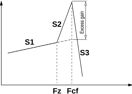
Figure 9: Their are 6 numbers that characterize every curve, three slopes ( ), in dB/oct, and two frequencies ( z

cf). Finally the excess gain characterizes the amount of gain at

cfrelative to the gain defined by . The Excess gain frequently depends on the input level for the case of a

nonlinear response like the cochlea.

2.1.1 Measures of cochlear response

There are two basic intertwined problems, cochlear frequency selectivity and cochlear

non-linearity. Whenever scientists are confronted with tangling (statistically correlated and

com-plex) phenomenon, good statistical measures are crucial. A measure called has been

popular, defined as the center frequency

cf divided by the bandwidth measured 10 dB

down from the peak. This measure is exquisitely insensitive to many important details and is difficult to accurately measure. Computing the bandwidth 10 dB down is subject to the error in estimating both the peak magnitude and the bandwidth. To compute , one must

subtract these two estimates, and then divide by this small quantity. Such manipulations are prone to large errors.

(18)

the literature.

Such Bode plots are useful for characterizing both cochlear selectivity and nonlinearity. By looking at the slope difference

(see Fig. 9 for the definitions of the slopes), we

have a statistic that is insensitive to the middle ear response. The slopes can be converted into the place domain by use of the cochlear map function. For example, in the cat where the conversion factor is 3 mm/oct, a slope of 6 dB/oct in the frequency domain is equivalent to 2 dB/mm. (The corresponding conversion factor for the human cochlea is 5 mm/oct.)

2.2 The nonlinear cochlea

Wegel and Lane’s transmission line theory is linear. Researchers began studying ways of making the cochlear models nonlinear in order to better understand these numerous nonlinear effects. Because these models are still under development (since the problem has not yet been solved), it is necessary to describe the data rather than the models.

Some of these important nonlinear cochlear measures include:

Distortion components generated by the cochlea, described by Wegel and Lane [81], Goldstein and Kiang [61], Smoorenburg [62], Kemp [75], Kim et al. [82], Fahey and Allen [83] (and many others),

The upward spread of masking (USM), first described quantitatively by Wegel and Lane in 1924,

Loudness growth and recruitment in the impaired ear [8],

The frequency dependent neural two–tone suppression observed by Sachs and Kiang [84], Arthur et al. [85], Kiang and Moxon [47], Abbas and Sachs [86], Fahey and Allen [83], [87] and others,

The frequency dependent basilar membrane response level compression first de-scribed by Rhode [46, 58], and,

the frequency dependent inner hair cell receptor potential level compression, first described by Russell and Sellick [55, 59].

The following sections review these data.

2.2.1 The basilar membrane nonlinearity

(19)

Figure 10: Figure 9a, panel B from Rhode (1978) showing the response of the basilar membrane for his most sensitive animal. The graduals along the abscissa are at 0.1, 1.0 and 10.0 kHz.

(20)

DATA TYPE Reference

2 cf

"

2

z! S1 S2 S3 Ex. Gain

octave dB/oct dB/oct dB/oct dB

BM [58] 0.57 9 92 107 27

BM [88] 0.88 10 30 101 17.4

Neural

2 cf

(kHz) [90] 0.5–0.8 0–10 50–170 300 50–80

Table 1: Summary of the parametric representation of basilar membrane (BM) and neural tuning from various sources. The parameters are defined in Fig. 9.

Fig. 10 (the most sensitive case), and his Table I, ,

9

, and

99

(dB/oct) (see Fig. 9 for the definitions), z = 5 kHz, cf = 7.4 kHz, and an excess gain of 27 dB.

(Rhode reported = 6 dB/oct, but 9 seems to be a better fit to the data, so 9 dB/oct is the

value we have used for our comparisons in Tab. 1.)

Very recent basilar membrane data from Narayan and Ruggero are shown in Fig. 11. In this figure we clearly see the nature of the nonlinear response growth and the change in frequency selectivity with input level.9 _{For this figure}

dB/oct between 0.3 and 9.0 kHz, while for the 20 dB SPL curve between 9.0 and 15.0 kHz is slightly less than 30

dB/oct,

= -101 dB/oct, z= 9 kHz,

cf= 16.6 kHz, and the excess gain is 20

. (600/80)

= 17.4 dB.

EPL CAT NEURAL TUNING DATA

1.0 97.0

-3.0

dB SPL

0.1 3.0 10.0

Fz

6.0 Fcf

FREQUENCY [kHz]

Figure 12: Cat neural tuning curves from Eaton Peabody Lab provided by C. Liberman and B. Delgutte. The pressure scale, in dB, has been reversed to make the curves look like filter transfer functions. The response “tail” for the 6 kHz neuron is the “flat” region between 0.1 kHz and frequency

z. In the tail the sound must be above 65 dB SPL (which on this scale is down) before the neuron

will respond.

2.2.2 Neural Tuning Data.

We ultimately seek a model which accurately predicts human inner hair cell and neural tuning curves. A great deal of cat VIII

neural tuning curve data are available which defines fairly precisely the input-output properties of the cochlea at threshold intensities.

(21)

Figure 13: Slopes of neural tuning curves for 8 different cats. The upper positive slopes, labeled

cfgive , the steep high frequency side of the tuning curve, while the negative slopes labeled

cfcorrespond to , the slope in the range of frequencies z cf. Above 2 kHz varies

from 50 to more than 100 dB/oct, while varies from about 50 dB/oct at 0.5 kHz to more than 400

dB/oct above 2-3 kHz. The numbers on each curve code different animals. This figure is Fig. 3 of reference [90].

Neural tuning is measured by measuring the spiking activity in an auditory nerve fiber as a function of the frequency and intensity of a probe search tone. The locus of threshold intensities

that cause the neuron to fire slightly above its spontaneous rate is called

the neural tuning curve. The superscript indicates that the probe intensity is at threshold.

Each neuron has such a tuning curve, which is tuned to its “best” characteristic frequency, labeled in Fig. 12 as cfand given by cfin Eq. 11. The tuning curves of Fig. 12 have been

vertically reversed to make them look more like the filter transfer functions used in basilar membrane response plots.

Tuning curve slopes. Those tuning curves having best frequencies cfabove a few kHz

typically have “flat tails,” meaning the broad flat region labeled as in Fig. 9 is less than 10

dB/oct. As an example look to the left of the frequency labeled FZfor the 7 kHz neuron of Fig. 12. For high frequency neurons ( cf 2 kHz), the slope in the tail 0. It is shown in

Fig. 13, is between 50-150 dB/oct,

300 dB/oct [90]. The excess gain is between 50-80 dB, and cf z 0.5 oct [91].

Tuning curve tips. Around the sensitive tips of tuning curves we expect the response to be similar to basilar membrane tuning, and there is significant evidence that this is the case [92, 88].

2.2.3 The receptor potential nonlinearity

(22)

nonlinear, especially at low sound pressure levels. They also greatly strengthened and clarified the case for the two–tone suppression nonlinearity observed in neural responses [84, 47, 86] which, due to neural saturation effects, was more difficult to quantify.

2.2.4 Motile OHCs

The implication that hair cells might play an important role in cochlear mechanics go back at least two 1936 when loudness recruitment was first reported by Fowler [93] in a comment by R. Lorente de No. [7], stating that cochlear hair cells are likely to be involved in loudness recruitment.

The same year Steinberg and Gardner (1937) were explicit about the action of recruit-ment when they concluded

When someone shouts, such a deafened person suffers practically as much discomfort as a normal hearing person would under the same circumstances. Furthermore for such a case, the effective gain in loudness afforded by am-plification depends on the amount of variable type loss present. Owing to the expanding action of this type of loss it would be necessary to introduce a corre-sponding compression in the amplifier in order to produce the same amplifica-tion at all levels.

Therefore as early as 1937 there was a sense that cochlear haircells were related to dy-namic range compression.

In more recent years, theoretical attempts to explain the difference in tuning between normal and damaged cochleae led to the suggestion that OHCs could influence BM me-chanics. In 1983 Neely and Kim conclude

We suggest that the negative damping components in the model may repre-sent the physical action of outer hair cells, functioning in the electrochemical environment of the normal cochlea and serving to boost the sensitivity of the cochlea at low levels of excitation.

Subsequently, Brownell et al. (1985) discovered that isolated OHCs change their length when placed in an electric field [57]. This then lead to the intuitive and widespread proposal that outer hair cells act as linear motors that directly drive the basilar membrane on a cycle by cycle basis. As summarized in Fig. 8, the length change was shown to be controlled by the outer hair cell receptor potential, which in turn is modulated by both the position of the basilar membrane (forming a fast feedback loop), and alternatively by the efferent neurons that are connected to the outer hair cells (forming a slow feedback loop). The details of this possibility are the topic of present research.

2.2.5 Low frequency suppressor effects

(23)

frequency) suppressor. These two views (USM versus 2TS) nicely complement each other, providing a symbiotic view of cochlear nonlinearity.

Upward Spread of Masking (USM). In a classic 1876 paper [95, 96], A.M. Mayer, was the first to describe the asymmetric nature of masking. Mayer made his qualitative ob-servations with the use of organ pipes and tuning forks, and found that that the spread of masking is a strong function of the probe-to-masker frequency ratio (

& ).

0 20 40 60 80

0 10 20 30 40 50 60 70

0.25 0.35 0.45

0.3 1

2

3

4

MASKER LEVEL (dB−SL)

MASKING (dB−SL)

MASKER AT 400 HZ

Figure 14: Masking from Wegel and Lane using a 400 Hz masker. The abscissa is the masker intensity in dB-SL. The ordinate is the threshold probe intensity

in dB-SL. The frequency

of the probe

, expressed in kHz, is the parameter indicated on each curve.

In 1923, Fletcher published the first quantitative results of tonal masking.10 _{In 1924,}

Wegel and Lane extended Fletcher’s experiments (Fletcher was the subject [17, Page 325]), using a wider range of tones. Wegel and Lane then discuss the results in terms of their 1 model described above. As shown in Fig. 14, Wegel and Lane’s experiments involved presenting listeners with a masker tone at frequency .& and intensity 8& , along

with a probe tone at frequency

. As a function of masker intensity (masker and probe frequency are fixed), the probe intensity

& was slowly raised from below-threshold

levels until it was just detected by the listeners, at intensity

& . As before indicates

threshold.

In Fig. 14 & = 400 Hz, & is the abscissa,

is the parameter on each curve, in kHz, and the threshold probe intensity

& is the ordinate. The dotted line superimposed on

the 3 kHz curve 8&

"

7

represents the suppression threshold at 60 dB-SL which has a slope of 2.4 dB/dB. The dotted line superimposed on the 0.45 kHz curve has a slope of 1 and a threshold of 16 dB SL.

(24)

Three regions are clearly evident: the downward spread of masking ( & , dashed

curves), critical band masking (

*& , dashed curve marked 0.45), and the upward

spread of masking (

& , solid curves) [98].

Critical band masking has a slope close to 1 dB/dB (the superimposed dotted line has a slope of 1). The downward spread of masking (the dashed lines in Fig. 14) has a low threshold intensity and a variable slope that is less than one dB/dB, and approaches 1 at high masker intensities. The upward spread of masking (USM), shown by the solid curves, has a threshold near 50 dB re sensation level (i.e., 65 dB SPL), and a growth just less than 2.5 dB/dB. The dotted line superimposed on the

=3 kHz curve has a slope of 2.4 dB/dB and a threshold of 60 dB.

The dashed box shows that the upward spread of masking of a probe at 1 kHz can be greater than the masking within a critical band (i.e.,

= 450 Hz & =400 Hz). As

the masker frequency is increased, this “crossover effect” occurs in a small frequency re-gion (i.e., 1/2 octave) above the masker frequency. The crossover is a result of a well documented nonlinear response migration, of the excitation pattern with stimulus intensity, described in a fascinating (and beautifully written) paper by Dennis McFadden [99]. Re-sponse migration was also observed by Munson and Gardner in a classic paper on forward masking [100]. This important migration effect is beyond the scope of the present discus-sion, but is is reviewed in [98, 101], and briefly described in the figure caption of Fig. 27.

The upward spread of masking is important because it is easily measured psychophysi-cally in normal hearing people, is robust, well documented, and characterizes the outer hair cell nonlinearity in a significant way. This psychophysically measured USM has correlates in basilar membrane, hair cell, and neural recording literature, where it is called two–tone suppression (2TS).

(25)

Two–tone suppression. The neural correlate of the psychophysically measured USM is called two–tone suppression (2TS). First a neural tuning curve is first measured. Next a pure tone probe at intensity

, and frequency

, is placed a few dB (i.e., 6 to 10) above threshold at the characteristic (best) frequency of the neuron cf(i.e.,

cf). Next

the intensity

of a suppressor tone, having frequency

, is increased until the rate response to the probe

either decreases by a small amount , or drops to

above the spontaneous rate

. These two criteria are defined (17)

(subscript s for superthreshold ) and

(18)

(subscript t for threshold ). indicates a fixed small but statistically significant constant

change in the rate (i.e., = 20 spikes/s is a typical value). The threshold suppressor

in-tensity is defined as

, and as before the indicates the threshold suppressor intensity.

The two threshold definitions

and

are very different, and both are useful.

Figure 16: The upper panel shows a family of neural tuning curves from the cat. The lower panel shows all the 2TS thresholds for this set of tuning curves. The circles are the locations of the

cfbias tone levels and frequencies. The solid lines are the intensity that will cause the suppressed tuning curve tip to be at the same level as that of the bias tone (the circle). The abscissa is in Pascals. 2 Pa is 100 dB SPL. The median suppression threshold at 1 kHz is 0.04 Pa (i.e., 66 dB SPL). For more details see [83].

Abbas and Sachs’ Fig. 8 [86] is reproduced in Fig. 15. For this example, cf is 17.8

kHz, and the

(26)

of the neural tuning curve was a low spontaneous neuron with a relatively high threshold of approximately 50-55 dB SPL. The left panel of Fig. 15 is for apical suppressors that are lower in frequency than the CF probe (

). In this case the threshold is just above 65 dB SPL. The suppression effect is relatively strong and independent of frequency. In this example the threshold of the effect is less than 4 dB apart (the maximum shift of the two curves) at suppressor frequencies

of 10 and 5 kHz (a one octave seperation). The right panel shows the case

. The suppression threshold is close to the neurons threshold (i.e., 50 dB SPL) for probes at 19 kHz, but increases rapidly with fre-quency.The strength of the suppression is weak in comparison to the case of the left panel (

), as indicated by the slopes of the family of curves.

The importance of the criterion. The data of Fig. 15 uses the first suppression thresh-old definition Eq. 17

(a small drop from the probe driven rate). In this case the cf

probe is well above its detection threshold at the suppression threshold, since according to definition Eq. 17, the probe is just detectably reduced, and thus audible. With the second suppression threshold definition Eq. 18

, the suppression threshold corresponds to the detection threshold of the probe. Thus Eq. 18, suppression to the spontaneous rate, is appropriate for Wegel and Lane’s masking data where the probe is at its detection thresh-old

& . Suppression threshold definition Eq. 18 was used when taking the 2TS data

of Fig. 16, where the suppression threshold was estimated as a function of suppressor frequency.

Figure 17: A cat neural tuning curve taken with various suppressors present, as indicated by the symbols. The tuning curve with the lowest threshold was with no suppressor present. As the suppressor changes by 20 dB, the _cf threshold changes by 36 dB. Thus for a 2 kHz neuron, the slope is 36/20, or 1.8. Interpolation of Fig. 18 gives a value of 1.6 dB/dB. One Pascal = 94 dB SPL.

(27)

curve pass through the cfprobe intensity of a 2TS experiment (i.e., be at threshold levels),

it is necessary to use the suppression to rate criterion given by Eq. 18. This is shown in Fig. 17 where a family of tuning curves is taken with different suppressors present. As described by Fahey and Allen (1985), when a probe is placed on a specific tuning curve of Fig. 17, corresponding to one of the suppressor level symbols of Fig. 17, and a suppression threshold is measured as shown in Fig. 16 (lower panel), that suppression curve will fall on the corresponding suppression symbol of Fig. 17. There is a symmetry between the tuning curve measured in the presents of a suppressor, and a suppression threshold obtained with a given probe. This symmetry only holds for criterion Eq. 18, the detection threshold criterion, which is appropriate for Wegel and Lane’s data.

Suppression threshold. Using the criterion Eq. 18, Fahey and Allen (1985) showed (Fig. 16) that the suppression threshold

in the tails is near 65 dB SPL (0.04 Pa).

This is true for suppressors between 0.6 and 4 kHz. A small amount of data are consistent with the threshold being constant to much higher frequencies, but the Fahey and Allen data are insufficient on that point.

Arthur et al. (1971), using Eq. 17, reported that when

the suppression threshold was more sensitive than the CF threshold. Fahey and Allen [83] used Eq. 18, and found no suppression for

, except for very high threshold neurons. This is because the rate never was suppressed to threshold for high frequency suppressors. For high frequency suppressors (

), suppression is a weak effect so it cannot suppress to threshold (Eq. 18) unless the neurons threshold is very high (greater than 60 dB SPL). This means that suppression above CF (

cf) can only be observed for low spontaneous, high

threshold neurons, when using Eq. 17.

Suppression slope. Bertrand Delgutte has written several insightful papers on masking and suppression [103, 102, 104]. As shown in Fig. 18, he estimated how the intensity growth slope (the ordinate, in dB/dB) of 2TS varies with suppressor frequency (the ab-scissa) for several probe frequencies (the parameter indicated by the vertical bar) [102]. As may be seen in the figure, the suppression growth slope for the case of a low frequency apical suppressors on a high frequency basal neuron (the case of the left panel of Fig. 15), is 2.4 dB/dB. This is the same slope as Wegel and Lane’s 400 Hz masker, 3 kHz probe USM data shown in Fig. 14. For suppressor frequencies greater than the probe’s (

), Delgutte reports a slope that is significantly less than 1 dB/dB. Likewise Wegel and Lane’s data has slopes much less than 1 for the downward spread of masking.

Related data. Kemp and Chum [105] (their Figs. 7 and 9) found similar suppression slopes of more than 2 dB/dB for low frequency suppressors of Stimulus frequency

emis-sions (SFE). This data seems similar to the USM and 2TS data, but is measured objectively

from the ear canal. New data on the suppression slope has been recently published by Pang and Guinan (1997).

In Fig. 19 Liberman and Dodds show the complex relationship between the state of the inner hair cell tuning and outer hair cell damage [43]. Local noise trauma to the outer hair cell produces tuning curves with elevated tips and increased sensitivity in the low frequency tails. There is a notch near z.

(28)

10−1 100 101 0

0.5 1 1.5 2 2.5 3

Suppressor Frequency (kHz)

Rate of growth of suppressor frequency

(29)

(30)

It is widely recognized that both the Liberman and Dodds as well as the Walsh and McGee [106] studies give us an important insight into micromechanics, but nobody has a simple explanation of exactly what these results mean. One likely possibility is that there are higher order modes (i.e., degrees of freedom) within the organ of Corti and the tectorial membrane.

Summary. The USM and 2TS data show systematic and quantitative correlations be-tween the threshold levels and slopes. The significance of this correlation has special importance because (a) it comes from two very different measurement methods, and (b) Wegel and Lane’s USM and Kemp’s SFE data are from human, while the 2TS data are from cat, yet they show quite similar responses. This implies that the cat and human cochleae may be quite similar in their nonlinear responses.

The USM and 2TS threshold and growth slope (e.g., 50 dB-SL and 2.4 dB/dB) are im-portant features that must be modeled before we can claim to understand cochlear function. While there have been several models of 2TS [107, 64, 108] as discussed in some detail by Delgutte [102], none are in quantitative agreement with the data. The two–tone suppres-sion model of Hall [64] is an interesting contribution to this problem because it qualitatively explores many of the key issues.

2.2.6 The basilar membrane to hair cell transformation

The purpose of this section is to address the two intertwined problems mentioned in Sec. 2.1.1,

cochlear frequency selectivity and cochlear nonlinearity,

A key question is the nature of the transformation between BM and hair cell cilia mo-tion at a given locamo-tion along the basilar membrane. There are several issues here. First, the motion of IHC and OHC cilia are not the same. The IHC cilia are believed to be free standing while the tips of OHC cilia are firmly anchored in the underside of the tectorial membrane. We may avoid this uncertainty by changing the question: What is the

trans-formation between BM and TM-RL shear? (Basilar membrane (BM), tectorial membrane

(TM) and reticular membrane (RL). The IHC and OHC cilia sit in the space between TM and RL.) The cilia sit in a 4-6 m fluid filled space between the tectorial membrane and the rectular lamina. It is the shearing motion between these two surfaces that moves the inner and outer hair cell cilia. The question reduces to the nature of the coupling between the vertical displacement of the BM and the radial shear of the TM-RL space. We dichotomize the possibilities into single versus multi-mode coupling. It is presently a matter of opinion as to which of these two couplings accounts for the most data.

Single-mode coupling. One possibility is that the displacement of the basilar membrane is functionally the same as the displacement of the TM-RL shear (and implicitly therefore the same as the OHC cilia). I will call this model single-mode coupling between the basilar membrane and the TM-RL shear. This means that the displacement magnitude and phase of these two displacements are significantly different. For example, they might differ by a linear transformation.

(31)

basilar membrane responses are functionally the same. The strongest argument for single-mode coupling is the study of [92] which is at one frequency and in one species. Even this data shows a small, systematic and unexplained 3.8 dB/oct difference across frequency.

Figure 20: Figure from Kim et al. 1979. The arrow indicates the frequency of the tone. The abscissa is the cfof each neuron, and the ordinate is the neural phase of the neuron relative to the

phase in the ear canal. Like the data of Fig. 19, this figure shows evidence for multi-mode coupling between the BM response and the cilia excitation.

Multi-mode coupling. The alternative to single-mode coupling is that neural signals are a multi-mode mechanics transformation of the basilar membrane response.11 There are many studies that are in conflict with single-mode coupling. There are at least two cate-gories of measurements that give insight into this transformation, tuning and nonlinearity. The following discussion summarizes many of the known differences between basilar mem-brane and neural response.

Noise damage. In my view Fig. 19 gives strong direct evidence of a tectorial membrane resonance (multi-mode “2 degrees of freedom” coupling). But this view has remained con-troversial. One problem with these data is the difficulty in interpreting them. But no matter what the interpretation, the data of Fig. 19 do not seem compatible with the concept of single-mode coupling.

Neural phase populations. As discussed extensively by this author on many occasions, phase measurements of the mechanical response and the neural response are fundamen-tally incompatible. Basilar membrane data has a monotonically lagging phase. Neural data

(32)

shows a 180 degree phase reversal at z (see Fig. 9), where the tip and tail meet in the

tuning curve, as shown at the 60% location along the basilar membrane (2 kHz place) in Fig. 20. The implication of this is that there is a well defined antiresonance (transmission zero) in the neural response at the frequency, where the tip and tail meet, that does not exist in the basilar membrane data.

Tuning curve slopes. Another line of reasoning comes from the cat neural tuning

curve slopes as seen in Tab. 1 and Figs. 12 and 16 for high frequency neurons. Slope for cat neural tuning curves having cf’s greater than 3 kHz are typically greater than 50

dB/oct. From Fig. 13, typical cat tuning curves in the 15 kHz range have slopes greater

than 100 dB/oct [90]. The slope of the basilar membrane response of Fig. 11 is 10 dB.

If we make a middle ear correction of -10 dB/oct (this is equivalent to a normalization with respect to ear canal pressure rather than incus displacement), the slope of Fig. 11 would

be =

-10 = 30-10 = 20 dB/oct.

Tuning curve “tails.” Neural tuning curve “tails” of high frequency neurons typically have threshold levels in excess of 65 dB SPL, as may be seen in Fig. 12 and Fig. 16.12 _The

slopes of neural responses in the tail are close to zero. Basilar membrane tuning curves do not have such tails.

BM versus neural 2TS. Recent basilar membrane 2TS measurements [111, 112, 108] have unequivocally shown that the neural and BM 2TS thresholds are significantly different. For example, Ruggero et al. (page 1096) says

. . . if neural rate threshold actually corresponds to a constant displacement ( 2 nm) . . . , then mechanical suppression thresholds would substantially exceed neural excitation thresholds and would stand in disagreement with findings on neural rate suppression.

Using a 0.1 nm displacement criterion, Cooper found basal excitation thresholds near 65 dB and 2TS thresholds near 85 dB SPL. Cooper says (page 3095, column 2, mid-paragraph 2)

Indeed, the direct comparisons shown . . . indicate that most of the low-frequency mechanical suppression thresholds were between 10 and 20 dB above the iso-displacement tuning curves . . . [corresponding] to “neural thresholds” at the site’s [CF].

That is, Cooper’s BM results placed the threshold of BM suppression about 1 order of magnitude higher in level than the Fahey and Allen 2TS thresholds shown in Fig. 16, both in absolute terms, and relative to the 0.1 nm threshold. The Geisler and Nuttall (1997) study [108] confirms these findings (see their Fig. 2).

BM versus other bandwidth estimates. BM displacement response are not in agree-ment with psychoacoustic detection experiagree-ments of tones in wide band noise, such as the

critical ratio experiments of Fletcher [36, 113], French and Steinberg [114], and Hawkins