FUZZIFIED DYNAMIC POWER
CONTROL ALGORITHM FOR
WIRELESS SENSOR NETWORKS
A.LAKSHMI* S.V. MANISEKARAN
Department of Information Technology, Assistant Professor,
Anna University of Technology Coimbatore, India. Department of Information Technology, Anna University of Technology Coimbatore, India.
DR.R.VENKATESAN
Professor, Department of Computer Science and Engineering, PSG College of Technology, Coimbatore, India.
Abstract :
This paper proposes novel energy efficient algorithm FDPCA for Wireless Sensor Networks (WSN). However, energy consumption is one of the major drawbacks in most of the Wireless Sensor Networks. Parameters like End to End Delay and Received Signal Strength Indicator (RSSI) are considered for exercising the influence on transmit power. These parameters are fuzzified and optimal transmission power levels are selected. The throughput for both DPCA and FDPCA are compared. High throughput is obtained by using FDPCA. In our first phase, the parameters are calculated. The proposed algorithm can effectively save energy without degrading the throughput of the network and reduce the energy consumption of the network. Our experimental results demonstrate that the proposed algorithm significantly overtake previous method, in terms of throughput.
Keywords: Wireless Sensor Networks (WSN), Dynamic Power Control Algorithm (DPCA), Received Signal Strength Indicator (RSSI), End to End Delay (EED), Throughput, Fuzzy Logic.
1. INTRODUCTION
Wireless Sensor Network (WSN) [1] are gaining fame across a diverse community due to their rich set of environmental information with an ample use in scientific applications. Sensor networks are a collection of sensor nodes, interconnected through wireless channels. The core function of the sensor nodes is to sense each node, gather the required data and to exchange data with its neighbors. These gathered data are stored in a centralized location.
WSNs involve a number of sensors, which have limited storage, low traffic rate, low mobility, high energy efficiency, predefined traffic patterns, processing capability and battery power [2]. These sensors can be either classified as static nodes or mobile nodes. In static sensor networks is based on routing algorithms on the lifetime of multi hop wireless sensor networks. All the data and control traffic in nodes the sensors will not move, they will be assigned a fixed location and sense environmental data. But in mobile nodes the sensor are not fixed, it will move from one location to another location and sense data. The Wireless Sensor Network uses its power wisely to extend their lifetime. Energy conservation plays a vital role in WSN [3]. Optimal placement of sensor nodes contributes to energy preservation.
2. RELATED WORK
reduced to a large extent without degrading the performance. It also extends the battery lifetime upto 30%. The location information is shared for each sensor nodes which controls transmit power.
The Location Aided Power Aware Routing (LAPAR) has been implemented in which location information is shared for each sensor nodes which controls the transmit power. The LAPAR can be implemented in any routing protocol. The optimum route between the source and destination are selected because the total power required for the transmission of data packets is minimized. Thus saves more power. Updates about location are a major drawback.
The energy efficient self-organization for wireless sensor networks is based on Time Division Multiple Access (TDMA) [6]. TDMA principles are incorporated in a new proposed protocol. In this protocol each sensor node is assigned a slot. The sensor utilizes its assigned slot only for sending data or receiving data, or else its receiver and transmitter are switched off. These sensor nodes are said to enter into any one of the two modes. They are idle/listen mode and sleep mode. The sensor node switches between both the modes based on its operations. When the sensors are not subjected to any other operation, they move on to the sleep mode. Wakeup packets are used to activate a sensor node from sleep mode to idle mode. It saves more power. Extensive simulations are involved in this protocol.
Similar to the wakeup protocol in wireless sensor networks, a single sleep schedule has been implemented [7]. This protocol eliminates some nodes to stay awake longer than the other. It improves energy efficiency and increases the life time of the sensor nodes. The main disadvantage of this protocol is high delay. The power efficiency in ad hoc and wireless sensor networks are based on routing algorithms on the lifetime of mutli hop wireless sensor networks. All the data and control traffic in the sensor networks are flowing between the sensor nodes and base station [8]. The lifetime bounds of the WSNs are calculated under specific routing algorithm. In this it minimizes the energy consumed for each node, due to the unnecessary overload some nodes die prematurely.
3.DPCA DETAILS
The Dynamic Power Control Algorithm (DPCA) is mainly applied for each and every individual links [9]. The parameter used here is Received Signal Strength Indicator (RSSI) . It reduces the interferences. The parameter is fuzzified. The Fuzzification process is mainly done to convert the ordinary values into fuzzy values. Based on its value the transmit power is calculated for the individual nodes. A large amount of energy is conserved by implementing DPCA. Inorder to increase the throughput a new Fuzzified Dynamic Power Control Algorithm is followed, which includes new parameters.
4. FDPCA DETAILS
The Fuzzified Dynamic Power Control Algorithm (FDPCA) is a modified version of DPCA in which new parameter is included. The variables used here are Received Signal Strength Indicator (RSSI) and End to End Delay (EED). The major advantage of using modified dynamic power control algorithm is increased network capacity, high throughput and reduced interferences.
A.FDPCA
Input : Data sensed by the node.
Output: Transmit power based on fuzzy decisions. For each node
Find the Received Signal Strength Indicator(RSSI) which ranges from 2mW to 15mW Find the End to End Delay (EED).
Calculate the average values. ARSSI=RSSI/n
AEED=EED/n
where n is the count, ARSSI and AEED are the average values Convert ordinary values into fuzzy values using s- Function. Store the fuzzy values.
Decide the transmit power based on the following conditions. If((RSSI==HI)&&(EED==HI or MED))
Pt=LOW
Pt=LOWMED
Else if((RSSI==MED)&&(EED==HI or MED)) Pt=MEDIUM
Else if((RSSI==MED)&&(EED==LOW)) Pt=HIMED
Elseif((RSSI==LOW)&&(EED==LOW or MED) Pt=HI
Else((RSSI==LOW)&&(EED==HI)) Pt=HIMED
End If
If number of errors >2, increase the Power Else
No change
Repeat the previous steps for every 5 seconds. End If
End for
The ranges selected for Fuzzy type variables: RSSI : HI >10mW
MED 5-10mW LOW <5mW EED: HI >10 MED 5-10 LOW <5 Pt: HI 0.28W HIMED 0.26W MED 0.24W LOWMED 0.22W LOW 0.20W
Each and every sensor node are sensed well for colleting the required data. These sensor nodes have some built in parameters like Topology, Channel Type, Energy Model, etc[10]. The two basic parameters are taken to perform calculations. They are Received Signal Strength Indicator (RSSI) and End to End Delay at each node. The Received Signal Strength Indicator (RSSI) are calculated from each node based on the transmitter power, receiver power, transmitter gain and receiver gain.
PRX=PTX..GTX.GRX.(λ/4πd)2 ---(1)
where,
PRX - Remaining power at the receiver
PTX - Transmission power
GRX - Gain of Receiver
GTX - Gain of Transmitter
λ - Wave Length
d - Distance between sender and receiver
RSSI=10.log (PRX/PRef) ---(2)
where,
PRef = 1
PRX - value is calculated from equation (1).
The End to End Delay (EED) is the ratio of the number of error to the total number of bits sent.
EED = Number of error .
Total number of bits sent. ---(3)
variables have a truth value that ranges between 0 and 1. The ordinary variables are converted into fuzzy type variables. This conversion is done by using s-function.
The fuzzification process is mainly done to group the parameters into different ranges like high, medium and low. If conditions are applied on these parameters to find the transmit power. Based on the transmit power and transmit time the total energy consumed is calculated. This mainly focuses on independent sensor modules that can operate without utilizing much power so that lifetime is extended.
B .Network Model
Lets take n sensor nodes which are randomly and uniformly distributed in a sensing field F and the sensor network has the following properties:
1. The sensor network model taken here is static. It means n sensor nodes are deployed in a two dimensional geographic space and these nodes do not move after deployment.
2. All nodes should be time coordinated on the order of seconds.
3. Nodes are location-aware, i.e. not equipped with GPS-capable antennae.
4. These nodes are uniformly distributed over the particular region and they are not mobile.
5.SIMULATION
The Fuzzified Dynamic Power Control Algorithm (FDPCA) is implemented using Network Simulator NS2. The energy consumed can also be calculated [11] as follows:
Energy Consumed = Σ( Pt * d ) where,
Pt - Transmit Power d - Transmit Time
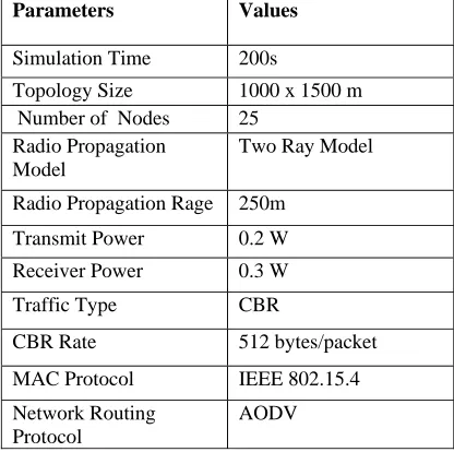
The following parameters are used for simulation .
Table 1: Simulation Parameters
Parameters Values
Simulation Time 200s
Topology Size 1000 x 1500 m Number of Nodes 25
Radio Propagation Model
Two Ray Model Radio Propagation Rage 250m
Transmit Power 0.2 W Receiver Power 0.3 W
Traffic Type CBR
CBR Rate 512 bytes/packet MAC Protocol IEEE 802.15.4 Network Routing
Protocol
Fig.1 NAM Screenshot of WSN with 25 nodes.
The simulation is done using ns 2.29 in windows environment by creating twenty-five sensor nodes. These sensor nodes are randomly arranged in 1000 x 1500 regions. The total energy is calculated for each and every sensor node. The Fuzzified Dynamic Power Control Algorithm (FDPCA) does not degrade the performance of the network in terms of end to end delay. The end to end delay for some nodes are calculated based on the received bytes and time.
Comparison is made between the DPCA and FDPCA algorithms in terms of throughput. FDPCA has higher throughput when compared to DPCA. The Throughput is calculated [12]. Throughput is the average rate of successful message delivery over the channel. It’s measured in bits per second or data packet per second / time slot.
Fig.2 Throughput comparison between DPCA and FDPCA.
6.CONCLUSION
REFERENCES
[1] [1] Holger Karl and Andreas Willig, “Protocols and Architectures for Wireless Sensor Networks”, First Edition, Wiley and sons, 2007.
[2] [2] IEEE 802.15.4a: Wireless Medium Access Control (MAC) and Physical Layer (PHY) Specifications for Low- Rate Wireless Personal Area Networks (WPANs), Internet draft.
[3] [3] Jagannathan Sarangapani , “Wireless Ad Hoc and Sensor Networks- Protocols, Performance And Control”, CRC Press, 2007. [4] [4] Sabitha Ramakrishnan, T.Thyagarajan, et. al, “Design and analysis of PADSR Protocol for routing in MANETs”, IEEE
International Conference INDICON 2005, pp.193-197, December 2005.
[5] [5] Sabitha Ramakrishnan and T.Thyagarajan, “Performance of PADSR protocol in MANETs with respect to network scaling”, International conference HiPAAC 2007”, July 2007.
[6] [6] Suyoung Yoon, Rudra Dutta, Mihail L. Sichitiu, “Power Aware Routing Algorithms for Wireless Sensor Networks”, Third International Conference on Wireless and Mobile Communications (ICWMC’07), 2007
[7] [7] Somnath Ghosh and Prakash Veeraraghavan, “Energy Efficient Medium Access Control with Single Sleep Schedule for Wireless Sensor Networks”, IEEE International Conference on Telecommunications and Malaysia International Conference on Communication, 14-17 May 2007, Penang, Malaysia.
[8] [8] Z. Chen, and A. Khokhar, “Self Organization and Energy Efficient TDMA MAC Protocol by Wake Up For Wireless Sensor Networks”, IEEE SECON 2004, August 2004.
[9] [9] Sabitha Ramakrishnan and T.Thyagarajan, “Energy Efficient Medium Access Control for Wireless Sensor Networks”, IJCSNS International Journal of Computer Science and Network Security, Vol. 9 No.6, June 2009.
[10] [10] Sabitha Ramakrishnan, T.Thyagarajan, et. Al, “A MAC-level Performance Enhancement Technique for
[11] Wireless Ad hoc / Sensor Networks”, Proceedings of the 6th International Conference TIMA 2009, pp. 264-268, January 2009. [12] [11] Javier Gomez and Andrew T. Campbell, “Variable-Range Transmission Power Control in Wireless Ad hoc Networks”, IEEE
transactions on Mobile Computing, Vol. 6, No. 1, pp. 87-99, January 2007.
[13] [12] Qingchun Ren and Qilian Liang, “Throughput and Energy-Efficiency-Aware Protocol for ultra wideband Communication in Wireless Sensor Networks: A Cross-Layer Approach”, IEEE Transactions On Mobile Computing, Vol. 7, No. 6, June 2008.
A.Lakshmi was born in Tamilnadu, India in 1988. She received her B.Tech degree in Information Technology from Anna University , Chennai in 2009. She is currently pursuing her final year M.Tech degree in Information Technology at Anna University of Technology Coimbatore. Her areas of interests are Networks and Software Engineering.
S.V.Manisekaran was born in Tamilnadu, India in 1981. He received his B.E. degree in Information Technology from Bharathiyar University, Coimbatore in 2003. He completed his M.E. in Computer Science and Engineering from Anna University Chennai in 2005. He is currently working as an Assistant Professor in the Department of Information Technology at Anna University Coimbatore, India. His research areas include mobile computing, quality management and software engineering.
Dr.R.Venkatesan was born in Tamilnadu, India, in 1958. He received his B.E (Hons) degree from Madras University in 1980. He completed his Masters degree in Industrial Engineering from Madras University in 1982. He obtained his second Masters degree MS in Computer and Information Science from University of Michigan, USA in 1999. He was awarded with PhD from Anna University, Chennai in 2007. He is currently Professor and Head in the Department of Computer Science and Engineering at PSG College of Technology, Coimbatore, India. His research interests are in Simulation and Modeling, Software Engineering, Algorithm Design, Software Process Management.