Cross-study validation for the assessment of prediction algorithms

Cross-study validation for the assessment of prediction algorithms

(Article begins on next page)

The Harvard community has made this article openly available.

Please share how this access benefits you. Your story matters.

Citation

Bernau, Christoph, Markus Riester, Anne-Laure Boulesteix,

Giovanni Parmigiani, Curtis Huttenhower, Levi Waldron, and

Lorenzo Trippa. 2014. “Cross-study validation for the assessment

of prediction algorithms.” Bioinformatics 30 (12): i105-i112.

doi:10.1093/bioinformatics/btu279.

http://dx.doi.org/10.1093/bioinformatics/btu279.

Published Version

doi:10.1093/bioinformatics/btu279

Accessed

February 16, 2015 10:40:49 AM EST

Citable Link

http://nrs.harvard.edu/urn-3:HUL.InstRepos:12406610

Terms of Use

This article was downloaded from Harvard University's DASH

repository, and is made available under the terms and conditions

applicable to Other Posted Material, as set forth at

http://nrs.harvard.edu/urn-3:HUL.InstRepos:dash.current.terms-of-use#LAA

Cross-study validation for the assessment of

prediction algorithms

Christoph Bernau

, Markus Riester

, Anne-Laure Boulesteix

, Giovanni Parmigiani

,

Curtis Huttenhower

, Levi Waldron

*

and Lorenzo Trippa

1

Leibniz Supercomputing Center, Garching,2Department for Medical Informatics, Biometry and Epidemiology, Munich, Germany, Cambridge, MA,3Dana-Farber Cancer Institute, Boston,4Harvard School of Public Health, Boston, USA and

5

City University of New York School of Public Health, Hunter College, New York, USA

ABSTRACT

Motivation:Numerous competing algorithms for prediction in high-dimensional settings have been developed in the statistical and ma-chine-learning literature. Learning algorithms and the prediction models they generate are typically evaluated on the basis of cross-validation error estimates in a few exemplary datasets. However, in most applications, the ultimate goal of prediction modeling is to pro-vide accurate predictions for independent samples obtained in differ-ent settings. Cross-validation within exemplary datasets may not adequately reflect performance in the broader application context.

Methods: We develop and implement a systematic approach to

‘cross-study validation’, to replace or supplement conventional cross-validation when evaluating high-dimensional prediction models in independent datasets. We illustrate it via simulations and in a col-lection of eight estrogen-receptor positive breast cancer microarray gene-expression datasets, where the objective is predicting distant metastasis-free survival (DMFS). We computed the C-index for all pair-wise combinations of training and validation datasets. We evaluate several alternatives for summarizing the pairwise validation statistics, and compare these to conventional cross-validation.

Results:Our data-driven simulations and our application to survival prediction with eight breast cancer microarray datasets, suggest that standard cross-validation produces inflated discrimination accuracy for all algorithms considered, when compared to cross-study valid-ation. Furthermore, the ranking of learning algorithms differs, suggest-ing that algorithms performsuggest-ing best in cross-validation may be suboptimal when evaluated through independent validation.

Availability:ThesurvHD: Survival in High Dimensionspackage (http:// www.bitbucket.org/lwaldron/survhd) will be made available through Bioconductor.

Contact:[email protected]

Supplementary information: Supplementary data are available at

Bioinformaticsonline.

1 INTRODUCTION

Cross-validation and related resampling methods are de facto

standard for ranking supervised learning algorithms. They allow estimation of prediction accuracy using subsets of data that have not been used to train the algorithms. This avoids over-optimistic accuracy estimates caused by ‘re-substitution’.

This characteristic has been carefully discussed in Molinaro

et al.(2005), Baek et al.(2009) and Simon et al. (2011). It is

common to evaluate algorithms by estimating prediction accur-acy via cross-validation for several datasets, with results sum-marized across datasets to rank algorithms (Boulesteix, 2013; Demsar, 2006). This approach recognizes possible variations in the relative performances of learning algorithms across studies or fields of application. However, it is not fully consistent with the ultimate goal, in the development of models with biomedical applications, of providing accurate predictions for fully inde-pendent samples, originating from institutions and processed by laboratories that did not generate the training datasets.

It has been observed that accuracy estimates of genomic pre-diction models based on independent validation data are often substantially inferior to cross-validation estimates (Castaldiet al., 2011). In some cases this has been attributed to incorrect appli-cation of validation; however even strictly performed cross-validation may not avoid over-optimism resulting from poten-tially unknown sources of heterogeneity across datasets. These include differences in design, acquisition and ascertainment stra-tegies (Simonet al., 2009), hidden biases, technologies used for measurements, and populations studied. In addition, many gen-omics studies are affected by experimental batch effects (Baggerly

et al., 2008; Leeket al., 2010). Quantifying these heterogeneities

and describing their impact on the performance of prediction algorithms is critical in the practical implementation of persona-lized medicine procedures that use genomic information.

There are potentially conflicting, but valid, perspectives on what constitutes a good learning algorithm. The first perspective is that a good learning algorithm should perform well when trained and applied to a single population and experimental set-ting, but it is not expected to perform well when the resulting model is applied to different populations and settings. We call such an algorithmspecialist, in the sense that it can adapt and specialize to the population at hand. This is the mainstream per-spective for assessing prediction algorithms and is consistent with validation procedures performed within studies (Baek et al., 2009; Molinaroet al., 2005; Simon et al., 2011). However, we argue that it does not reflect the reality that ‘samples of conveni-ence’ and uncontrolled specimen collection are the norm in gen-omic biomarker studies (Simonet al., 2009).

We promote another perspective: a good learning algorithm should begeneralist, in the sense that it yields models that may be suboptimal for the training population, or not fully representa-tive of the dataset at hand, but that perform reasonably well

*To whom correspondence should be addressed.

y_{The authors wish it to be known that, in their opinion, the last two}

authors should be regarded as Joint Last Authors.

across different populations and laboratories employing compar-able but not identical methods. Generalist algorithms may be preferable in important settings, for instance when a researcher develops a model using samples from a highly controlled envir-onment, but hopes the model to be applicable to other hospitals, labs, or more heterogeneous populations.

In this article we systematically use independent validations for the comparison of learning algorithms, in the context of microarray data for disease-free survival of estrogen receptor-positive breast cancer patients. Although concern has been often expressed about the lack of independent validation of gen-omic prediction models (Micheelet al., 2012; Subramanian and Simon, 2010), independent validation has not been systematically adopted in the comparison of learning algorithms. This defi-ciency cannot be addressed for prediction contexts where related, independent datasets are unavailable. For many cancer types, however, several micro-array studies have been performed to develop prognostic models. These datasets pave the way for a systematic approach based on independent validations. For in-stance, a recent meta-analysis of prognostic models for late-stage ovarian cancer provides a comparison of publicly available microarray datasets (Waldron et al., 2014). Furthermore, Riester et al. (2014) showed that combining training datasets can increase the accuracy of late-stage ovarian cancer risk models. Thus situations exist in genomic data analysis where comparable, independent datasets are available, and these pre-sent an opportunity to use independent validation as an explicit basis for assessing learning algorithms.

We propose what we term ‘leave-one-dataset-in’ cross-study validation (CSV) to formalize the use of independent validations in the evaluation of learning algorithms. Through data-driven simulations, and an example involving eight publicly available estrogen receptor-positive breast cancer microarray datasets, we assess established survival prediction algorithms using our ‘leave-one-dataset-in’ scheme and compare it to conventional cross-validation.

2 METHODS

2.1 Notation and setting

>We consider multiple datasetsi= 1,. . .,Iwith sample sizesN1,. . .,NI. Each observationsappears only in one dataseti, i.e. datasets do not over-lap, and the corresponding record includes a primary outcomeYs

iand a

vector of predictor variablesXs

i;throughout this articleXsi will be

gene-expression measurements. Our goal is to compare the performance of dif-ferent learning algorithmsk= 1,. . .,Kthat generates prediction models for the primary outcome using the vector of predictors. Throughout this article, the primary outcome is a possibly censored survival time.

We are interested in evaluating and ranking competing prediction methodsk= 1,. . .,K. Since the ranking may depend on the application, the first step is to define the prediction task of interest. We focus on the prediction of metastasis-free survival time in breast cancer patients based on high-throughput gene-expression measurements. Our approach and the concept of CSV, however, can be applied to different types of re-sponse variables and any other prediction task.

2.2 Algorithms

We assess six learning algorithms (k= 1,. . ., 6) appropriate for high-dimensional continuous predictors and possibly censored time-to-event

outcomes:LassoandRidge regression(Goeman, 2010),CoxBoost(Binder and Schumacher, 2008),SuperPC(Blair and Tibshirani, 2004),Unicox

(Tibshirani, 2009) andPlusminus(Zhaoet al., 2013). All parameters were tuned either by default methods included in their implementation (Ridge and Lasso regression: R-package glmnet) or by testing a range of param-eters in internal cross-validation. Our focus is not to provide a compre-hensive array of algorithms, but simply to use a few popular, representative algorithms to investigate CSV.

2.3 CSV matrices

We refer in this article tom-fold cross-validation and related resampling methods collectively as cross-validation (CV). Our ranking procedure for learning algorithms is based on a square matrix Zk of scores (k= 1,. . .,K). The (i,j) element in the matrix measures how well the model produced by algorithmk trained on dataseti performs when validated on datasetj. Since we considerKmethods we end up withK

method-specific square matricesZ1;. . .;ZK:We set the diagonal entries of the matrices equal to performance estimates obtained with 4-fold CV in each dataset. We will callZktheCSV matrix.

Possible definitions for theZki;jscores include the concordance index in

survival analysis (Harrellet al., 1996), the area under the operating char-acteristic curve in binary classification problems, or the mean squared distance between predicted and observed values in regression problems.

We use survival models and focus on a concordance index, the C-index, which is a correlation measure (Gnen and Heller, 2005) between survival times and the risk scores, such as linear combinations of the predictors, provided by a prediction model. The heatmap in Figure 1A displays theCSVmatrix of C-statistics obtained through validation of eight models trained on the studies in Table 1 withRidge regression.

2.4 Summarization of a CSV matrix

In order to rank learning algorithmsk= 1,. . .,K, we summarize each matrix Zk by a single score. We consider following two candidate approaches.

(1) TheSimple Averageof all non-diagonal elements of the Zkmatrix:

CSV= X i X i6¼j Zk_i;j IðI1Þ :

(2) The Median or more generally a quantileof the non-diagonal entries ofZk. Quantiles offer robustness to outlier values, and the possibility to reduce the influence of those studies that are consistently associated with poor validation scores, both when used for training and validation, and independently of the learning algorithm.

2.5 True global ranking

Throughout our analyses the scoreZk

i;jis a random variable. First, studies

iandjcan be seen as randomly drawn from a population of studies. Second, observations within each study can be considered as randomly drawn from the unknown and possibly different distributionsFiandFj underlying studiesiandj. With this view ofZk

i;jas random variable, we

consider the theoretical counterparts of the empirical aggregating scores (simple average and quantiles) described in Section 2.4 to summarizeZk. The theoretical counterparts are the expected value or quantiles of each

Zk_i;jscore,i6¼j;obtained by integrating the two levels of randomness that we described. The true global ranking of the learning algorithms

k= 1,. . .,Kis then defined by these expected values (or quantiles), one for each algorithm. We will call the rankingglobalbecause it depends on the super-population (Hartley and Sielken, 1975) and not which popula-tions were sampled by the available datasets.

i106

The true global ranking can be considered as the estimation target of evaluation procedures such as CV or CSV. In Section 2.7 we present the design of a data-driven simulation study in which we can compute the true ranking through Monte Carlo integration. This allows us to evaluate and compare the ability of CV and CSV to recover the true global ranking.

2.6 Datasets

We used a compendium of breast cancer microarray studies curated for the meta-analysis of Haibe-Kainset al.(2012) and available as supple-ment to their article. We selected all eight datasets (Table 1) for which distant metastasis-free survival (DMFS), the most commonly available time to event endpoint, as well as Estrogen Receptor (ER) status, were

available. These studies were generated with Affymetrix HGU GeneChips HG-U133A, HG-U133B and HG-U133PLUS2. We con-sidered exclusively ER-positive tumors. Of these datasets, only one origi-nated from a population-based cohort (Schmidtet al., 2008). Four studies considered only patients who did not receive hormone therapy or adju-vant chemotherapy. Only four provided date ranges of patient recruit-ment (Chin et al. 2006; Desmedt et al., 2007; Foekens et al., 2006; Schmidtet al., 2008). Table 1 points also to important differences in survival (for instance 3Q survival) that are not easily explicable based on known characteristics of these studies. This variability in design stra-tegies, reporting, as well as outcomes, highlights the prevalence of ‘sam-ples of convenience’ in biomarker studies discussed by Simonet al.(2009). Samples from dataset ST1 duplicated in dataset VDX were removed. Expression of each gene was summarized using the probeset with

A B C

Fig. 1.CSV matricesZkin simulated and experimental data forRidge regression.(A)C-indices for training and validation on each pair of actual datasets in Table 1. The diagonal of this matrix shows estimates obtained through 4-fold CV.(B)The heatmap for each pair of studies (i,j), the average C-index when we fitRidge regressionon a simulated dataset generated by resampling gene expression data and censored time to event outcomes from thei-th study in Table 1, and validate the resulting model on a simulated dataset generated by resampling studyj. Computation of each diagonal element averages over pairs of independent datasets obtained by resampling from the same study. The heatmaps strongly resemble each other. CAL and MSK are outlier studies: cross-study C-index is0.5 when they are used either for training or validation. The values of the arrays in (A) and (B) that involve these two studies constitute the blue ‘bad performance’ cluster in(C)which contrast the C-indices obtained for study pairsði;jÞ;i6¼j, on simulated data (y-axis) and experimental data (x-axis). Pearson correlation is0.9. The three plots illustrate similarity between our simulation model and the actual datasets in Table 1

Table 1.Breast cancer microarray datasets curated by Haibe-Kainset al.(2012)

Number Name Adjuvant therapy

Number of patientsa

Number of ER+ 3Q survival [mo.] Median follow-up [mo.] Original identifiersb Reference

1 CAL Chemo, hormonal 118 75 42 82 CAL Chinet al.(2006) 2 MNZ none 200 162 120 94 MAINZ Schmidtet al.(2008) 3 MSK combination 99 57 76 82 MSK Minnet al.(2005) 4 ST1 hormonal 512a 507b 114 106 MDA5, TAM, VDX3 Foekenset al.(2006) 5 ST2 hormonal 517 325 126 121 EXPO, TAM Symmanset al.(2010) 6 TRB none 198 134 143 171 TRANSBIG Desmedtet al.(2007) 7 UNT none 133 86 151 105 UNT Sotiriouet al.(2006)

8 VDX none 344 209 44 107 VDX Minnet al.(2007)

Datasets acronyms: CAL, University of California, San Francisco and the California Pacific Medical Center (USA); MNZ, Mainz hospital (Germany); MSK, Memorial Sloan-Kettering (United States). ST1 and ST2 are meta-datasets provided by Haibe-Kainset al.(2012), TRB denotes the TransBIG consortium dataset (Europe), UNT denotes the cohort of untreated patients from the Oxford Radcliffe Hospital (UK), VDX = Veridex (the Netherlands). Number of ER+ is the number of patients classified as Estrogen Receptor positive. 3Q survival indicates the empirical estimate of the 75-th percentile of the distribution of the survival times (in months). Median follow-up (in months) is computed using the reverse Kaplan–Meier estimate to avoid under-estimation due to early deaths (Schemper and Smith, 1996).a

Numbers shown are after removal of samples duplicated in the dataset VDX.b

maximum mean (Miller et al., 2011). The 50% of genes with lowest variance were removed. Subsequently, gene-expression values were scaled by linear scaling of the 2.5 and 97.5% quantiles as described by Haibe-Kainset al.(2012).

2.7 Simulation design

We simulate heterogeneous datasets with gene-expression profiles and time to event outcomes from a joint probability model. We define the model through a resampling procedure that we apply to the eight breast cancer datasets in Table 1. The resampling scheme is a combination of parametric and nonparametric bootstrap (Efron and Tibshirani, 1993). The goal of our simulation study is to compare CV and CSV when used for ranking and evaluation of competing learning algorithms. Here we use resampling methods to iteratively simulate realistic ensembles of breast cancer datasets from a hierarchical probability model that we define using the actual datasets in Table 1. CV and CSV are then assessed with respect to their ability to recover the true global ranking, which we compute through Monte-Carlo integration.

We will quantify the ability to recover the ranking by using the Kendall correlation between the true global ranking and the estimates obtained with CV or CSV.

Forb= 1,. . .,B= 1000 iterations, we generate a collection ofI= 8 datasets as follows. First, we sample eight study labels with replacement from the list of breast cancer studies in Table 1. This step only involves simulations from a multinomial Mult(8,[1/8,. . ., 1/8]) distribution. We resample the collection of study labels to capture variability in study availability, and heterogeneity of study characteristics. Second, for each of the eight randomly drawn labels, we sampleN= 150 patients from the corresponding original dataset, with replacement. If a study is randomly assigned to thej-th label, then each of theN= 150 vectors of predictive variables is directly sampped from the empirical distribution of thej-th study in Table 1. Finally, we simulate the corresponding times to event using a proportional hazards model (parametric bootstrap) fitted to the

j-th dataset: Mjtrue:jðtjxÞ= j 0ð Þ t expxTj ; ð1Þ wherej_(t

jx) is the individual hazard function when the vector of pre-dictors is equal toxandjdenotes a vector of regression coefficients. We

combine the truncated inversion method in Benderet al.(2005) and the Nelson–Aalen estimator for cumulative hazard functions to simulate sur-vival times that reflect sursur-vival distributions and follow-up of the real studies. We set the vectorjto be the coefficients fitted in studyj= 1,. . .,

Iusing theCoxBoostmethod (Binder and Schumacher, 2008). A different regression method could have been used at this stage. The collections of simulated datasets are then used both (i) to compute by Monte-Carlo method the true global ranking defined in Section 2.5, and (ii) to compute ranking estimates through CV and CSV. Figure 1A displays, for each pair of studies (i,j) in Table 1, the C-index obtained when training a model by

Ridge regressionon dataseti(rows), and validating that model on dataset

j(columns). We computed the diagonal elements (i=j) by 4-fold CV. Figure 1B displays mean C-indices for each (i, j) combination across simulations, when the training and validation studies are generated resampling thei-th andj-th study. Here diagonal elements are computed by averaging C-indices with the training and validation datasets inde-pendently generated by resampling from the same study.

The strong similarity between the two panels is reassuring, in particular with regard to the clear separation of the eight studies into two groups. The first group includes studies MNZ, ST1, ST2, TRP, UNT and VDX, and produces more accurate prediction models than the remaining stu-dies. The datasets in this group are also associated with higher values of the concordance index when used for validation. This difference between the two groups is also illustrated in Figure 1C. It displays the non-diag-onal entries of the matrices represented in the left and middle panels, that is the average C-indices from simulated datasets, against the C-indices

from real data. This scatterplot shows a clear two-cluster structure: the yellow dots display the 30 training and validation combinations within studies MNZ, ST1, ST2, TRP, UNT and VDX. We will return to this cluster structure in the discussion.

2.8 Evaluation criteria for simulations

In simulation studies we can assess and rank algorithms based on their ability to recover the true underlying modelsMi

true;i=1;. . .;I:In this subsection, we introduce a criterion that reflects the degree of similar-ity between the true regression coefficients i that were used to

simulate thei-thin silicodataset and the coefficientsbðkÞ_j fitted through algorithmkon thej-th simulated dataset. We consider thei=jandi6¼j

cases separately. Similarity between vectors is usually quantified by com-puting the Euclidean distance between them. However, since our focus is on prediction, we use

c

corðXii;Xib ðkÞ

j Þ;the correlation between true and estimated

patient-specific prognostic scores, to measure the similarity between the truei

and estimated regression coefficientsbðkÞ_j :HereXiis the matrix of pre-dictors of datasetiandcor denotes Pearson’s correlation. The averagec

Sk self= 1ð =IÞ X i c cor Xii;Xib k ð Þ i ; ð2Þ

over theIstudies, provides a measure of the ability of learning algorithm

kto recover the model that has generated the training dataset, hence the indexself.

Another criterion of interest is the ability of a learning algorithmkto recover the vector of regression coefficientsi when it is trained on a

separate datesetj6¼iand the unknown models underlying datasetsiandj

might differ from each other. This can be quantified with

Sk across= 1ð =ðI Ið 1ÞÞÞ X i X j6¼i c cor Xii;Xib k ð Þ j ; ð3Þ

where the indexacrossemphasizes the focus on cross-study similarity, i.e. on the ability of algorithmkto recover the coefficientsiwhen fitted on

datasetj, withj6¼i:

In alternative to averaging across studies, or pairs of datasets, as in Equations (2–3) one can also use different summaries, e.g. quantiles, as we do in Section 2.4. BothSk

selfandSkacrossare summary statistics to assess and compare learning algorithms. We denote the ranking obtained by ordering the algorithms according toSself(Sacross) byRself(Racross). Both

Sk

self andSkacross vary across simulations of the datasets ensembles, al-though the hierarchical simulation model remains fixed and their com-putations involve the vectors_i,i= 1,. . .,I. We will therefore call the rankingsRselfandRacrosslocalbecause they are specific to the collection

of datasets at hand.

3 RESULTS

3.1 Simulated data

Our focus in the simulation study is on differences between the rankings and performance estimates obtained by using CV and CSV. We will use CV and CSV to denote the means of the diagonal and non-diagonal elements of a CSV matrix, respect-ively. Recall that we compute the diagonal elements through CV. Figure 2A shows, forK= 6 algorithms, the distributions of CSV and CV;and Figure 2B shows the distribution of the rank-ings estimates, across 1000 simulated collections of eight data-sets. Table 2 compares the medians of the distributions in Figure 2B with the true global rankings that we obtained using the criteria in Section 2.4. The rank of method k is 1 if it

i108

outperforms the remainingK– 1 training algorithms. We ob-serve large differences in the distributions of CSV and CV across simulations (Fig. 1A): the average of the CV scores, under all the algorithms we considered, is close to 0.65, while the CSV scores are centered at0.55. The variability of CV and CSV across simulations, however, is comparable.

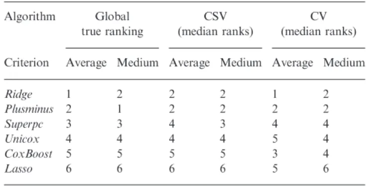
Performance differences across algorithms, whether estimated by CV or CSV, are relatively small compared to the overall dif-ference between CV and CSV performance estimates. We also observe differences between the rank distributions produced by CV and CSV. Accordingly, to both CV and CSV, in most of the simulations,Lasso regressionis ranked as one of the worst per-forming algorithms, whileRidge regression and Plusminus are ranked first or second. However, the CV summaries suggest an advantage ofRidge regressionoverPlusminusacross most of the simulations while CSV rankPlusminusas the best performing algorithm in 50% of the simulations. The median rank of

CoxBoostacross simulations has an improvement of two

pos-itions when it is estimated through CV and compared to the CSV summaries; in this case CSV results are more consistent with the true global rankings (Table 2). When we consider the criteria described in Section 2.4, Ridge regression and Plusminus ex-change the top-two positions of the true global rankings (see Table 2), although for these two algorithms theZi,jdistributions under our simulation scenario are nearly identical.

The local rankings Racrossand Rselfof the K= 6 algorithms

defined bySk

across and Skself in Section 2.8 vary across the 1000

simulated collections of studies. The median Kendall’s correl-ation betweenRacross and Rself across simulations is 0.5, i.e. the performance measuresSk

acrossandSkselftend to define distinct

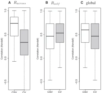
rankings of the competing algorithms, see also the Supplementary Figure S1. We illustrate the extent to which CV and CSV recover the unknown rankingsRacross andRself. The

boxplots in Figure 3 display the Kendall’s correlation between local rankings (i)Racrossor(ii)Rself, and the rankings estimated through CV (gray boxes) and CSV (white boxes) across simula-tions. Figure 3C shows the Kendall’s correlation between the true global ranking and the ranking estimates. The median Kendall’s correlation betweenRselfand the corresponding CSV estimates across simulations is0.5. The CV ranking estimates tend to be less correlated with the local rankingsRacrossthan the CSV estimates. In contrast, the CV estimates tend to be more correlated withRselfthan the CSV estimates. We recall that both CV and Rself are defined summarizing performance measures, Zk_i;i and cor_cðXii;Xib

ðkÞ

i Þ; that refer to a single study, while

CSV and Racross summarizes performance measures computed using two distinct studies that are used for training and validation.

Finally, CSV tends to be more correlated with the true global ranking than CV. This suggests that CSV is more suitable for recovering the true global ranking. When we removed the two outlier studies (CAL and MSK) and repeated the simulation study, the advantage of CSV over CV in recovering the true global ranking was confirmed (median Kendall’s correlation 0.8 versus 0.6, see also Supplementary Figs S2–S4), moreover after their removal Kendall’s correlations betweenRselfand the CSV estimates tend to be larger than those betweenRselfand the CV estimates. Overall, as displayed by the Supplementary Figure S3, it appears that, after outlier studies are removed, CSV out-performs substantially CV when used for ranking algorithms.

3.2 Application to breast cancer prognostic modeling

We apply CV and CSV to the I= 8 breast cancer studies described in Section 2. Generally, the results resemble those ob-tained on simulated data. The top panel in Figure 4 illustrates the distributions of the diagonal and off-diagonal validation statis-tics inZkfor each of the K= 6 algorithms. Except for the dis-tinctly larger interquartile ranges of the box-plots we observe several similarities with Figure 2. Note that each box-plot A

B

Fig. 2.Comparison of CSV and CV on simulated data. Each panel rep-resents evaluations ofK= 6 algorithms across 1000 simulations of a compendium ofI= 8 datasets. For each simulation the diagonal or off-diagonal elements of theZkmatrix of validation C-statistics is sum-marized by(A)mean and(B)rank of the mean across algorithms. CV estimates tend to be much higher than the CSV estimates. In most of the simulations Lasso is ranked as one of the worst algorithms, both by CV and CSV, whileRidgeandPlusminusare ranked among the best predic-tion methods

Table 2. True global rankings and estimates with CV and CSV on simulated data Algorithm Global true ranking CSV (median ranks) CV (median ranks) Criterion Average Medium Average Medium Average Medium

Ridge 1 2 2 2 1 2 Plusminus 2 1 2 2 2 2 Superpc 3 3 4 3 4 4 Unicox 4 4 4 4 5 4 CoxBoost 5 5 5 5 3 4 Lasso 6 6 6 6 5 6

Median estimates across 1000 simulations are displayed for CV and CSV; individual columns refer to summarization of theZk

i;j statistics by using the mean or the

median as discussed in Section 2.4. We also computed the true global ranking as well as CV and CSV estimates by using the third quartile of theZk

i;jsummaries, and

obtained results identical to those displayed for the rankings obtained by summar-izing validation results through their median. Both CV and CSV tend to rankRidge regressionandPlusminusas best performing algorithms. Variability of CV and CSV rank estimates across simulations is shown in Figure 2B.

represents validation scores within a singleZk-matrix, whereas in Figure 2 each box-plot displays a summary of 1000Zkmatrices, one for each simulation. This explains the higher variance observed in Figure 4. We also observe the following.

CV estimates are0.06 higher than CSV estimates on the C-index scale. To interpret the magnitude of this shift on the C-index scale consider a population with two groups of pa-tients, high and low risk papa-tients, covering identical propor-tions 0.5 of the population. Aperfect discrimination model

that correctly recognizes the subpopulation of each individ-ual, when the hazard ratio between high versus low risk patients is 2.7, achieves on average a C-index of 0.62. It is necessary to double the hazard ratio to 5.4 to increase the average C-index of the perfect discrimination model to 0.68. Thus, it is fair to say that the CV results are considerably more optimistic than the CSV estimates.

The ranking defined by CSV, using median summaries of theZk_i;jscores, is nearly identical to the global ranking in our simulation example (see Supplementary Table ST1 and Table 2). With both, median and third quartile aggregation of the Zk_i;jstatistics, the rankings defined by CV and CSV differ substantially (Kendall’s correlations 0.6 and 0.07). This is consistent with the results of the simulation study, where median correlation of the rankings estimated through CSV and CV was0.4 (see Supplementary Fig. S1). The presence of outlier studies (CAL and MSK) has a

strong effect on the ranking estimates when we use the mean to summarize theZkmatrices. After aggregating the validation statistics by averaging, both CSV and CV rank

Superpcfirst. This result might be due to the high variability,

0.5, of theZk_i;jvalidation scores corresponding to models trained by outlier studies. In particular,SuperpcandUnicox

are the only algorithms that produce models with substantial prediction performances when trained on the MSK study. With median summarization the ranking estimates are less influenced by the presence or absence of outlier studies. We therefore recommend the use of the median to summarizeZk matrices.

Figure 4B illustrates lack of agreement between CSV and CV performance estimates. The black digits contrast, for each dataseti, the CSV summaryX

j6¼iðI1Þ

1_Zk i;jversus

the CV summaryZk_i;i:Performance measures refer toRidge

regression. Similarly, the gray digits in this panel contrast

X

j6¼iðI1Þ

1

Zk_j;i with Zk_i;i: The CV performance statistics Zk_i;i are only moderately correlated with the CSV statistics X

j6¼iðI1Þ

1_Zk

i;j (correlation = 0.2), and

negatively correlated with the CSV summaries X

j6¼iðI1Þ

1_Zk

j;i(correlation = –0.33).

3.3 CV and CSV summaries

Correlation between CSV and CV summary statistics, as dis-played in Figure 4B, suggests that cross- and within-study per-formances are less redundant than one might expect. In Figure 4B study specific CSV summaries are plotted against CV for Ridge regression. For each study we have a single CV statistic and two CSV statistics obtained by averaging the

A

B

Fig. 4.Panel(A)describes the CSV and CV statistics inZk, separately for each of the six algorithms that we considered. Each box-plot represents the variability of CV or CSV performance statistics from a singleZk

matrix. The CV statistics tend to be higher than the CSV statistics. Panel(B)contrasts with black digits, for each studyi, the CSV summary X

j6¼iðI1Þ 1

Zki;jwith the CV summaryZki;i:Similarly, with gray digits

it contrasts the CSV summaryX

j6¼iðI1Þ 1

Zkj;iwith the CV summary Zk

i;i:This panel shows results for the learning algorithmRidge regression

and the displayed numbers refer to Table 1 (outliers CAL and MSK were removed). Cross-validation statistics on they-axis are moderately corre-lated to the CSV summaries on thex-axis; identical considerations hold for allK= 6 algorithms that we used

A B C

Fig. 3.Kendall’s correlation between true global or local rankings and estimates obtained with CSV (white box-plots) or CV (cross-validation, gray box-plots) across simulations. Panels(A)and(B)compare CV and CSV in terms of their correlation to thelocal rankings(RacrossandRself),

while panel(C)considers the true global ranking. Each box-plot repre-sents a correlation coefficient that was computed in each of the 1000 iterations of our simulation study. CSV tend to achieve a higher correl-ation with the global ranking andRacrossthan CV. The results displayed

have been computed using the mean criterion discussed in Section 2.4

i110

Z-matrix column- and row-wise. In the column-wise case correl-ations, between CSV and CV summaries, vary across algorithms 0.5, while in the row-wise case all the correlations are negative. Overall, we can consider cross- and within-study prediction as two related but distinct problems.

We also noted that CV is less suitable for detection of outlier studies than CSV; in particular CV can estimate encouraging prediction performances even on studies associated, under each training algorithm, with poor CSV summariesZk_i;i:For instance, with the SuperPCalgorithm all but one C-index estimates ob-tained with CV are above 0.6.

3.4 Specialist and generalist algorithms

Our analyses lead to the question of whether some algorithms can be considered as generalist or specialist procedures according to our definitions. Our examples are not exhaustive and add-itional comparisons, within the development of new prognostic models, are necessary in order to determine ‘specialist’ or ‘gen-eralist’ tendencies of these algorithms. However, the fact that

Ridge regression,Lasso regressionandCoxBoostare ranked

dis-tinctly better accordingly to CV than CSV, in most iterations of our simulation study, suggests that these algorithms might be specialist procedures and adapt to the specific properties of the individual dataset. The status of generalist versus specialist, for each algorithm, can be discussed using the local performance criteria Sself and Sacross, which are conceived to measure within-single-studies and generalizable prediction performances. We note that CoxBoost and Ridge regression tend to achieve better ranks inRselfthan inRacross. In particularCoxBoost im-proves its position by 1 or 2 ranks in most simulations, which is similar to what we observed comparingCoxBoost’s CSV and CV rankings. In summary, in our study, these two algorithms seem to have—accordingly to all the criteria that we considered—a tendency to specialize to the dataset at hand. We mention that, as one can expect, for all the algorithms Sself is consistently higher than Sacross. We also compared CV to independent

within-study validationusing our simulation model. For the

inde-pendent within-study validation, we iteratively pair two datasets generated using identical regression coefficients and gene expres-sion distributions. Subsequently, we train a model on the first dataset and evaluate it on the second one. As can be seen in Supplementary Figure S5, CV values, as expected, are slightly smaller than for the independent within-study validations.

4 DISCUSSION AND CONCLUSION

In applying genomics to clinical problems, it is rarely safe to assume that the studies in a research environment faithfully rep-resent what will be encountered in clinical application, across a variety of populations and medical environments. From this standpoint, study heterogeneity can be a strength, as it allows to quantify the degree of generalizability of results, and to inves-tigate the sources of the heterogeneity. This aspect has long been recognized in meta-analysis of clinical trials (Moher and Olkin, 1995). Therefore, we expect that an increased focus on quantify-ing cross-study performance of prediction algorithms will con-tribute to the successful implementation of the personalized medicine paradigm.

In this article we provide a conceptual framework, statistical approaches and software tools for this quantification. The con-ceptual framework is based on the long-standing idea that finite populations of interest can be viewed as samples from an infinite ‘super-population’ (Hartley and Sielken, 1975). This concept is especially relevant for heterogeneous clinical studies originating from hospitals that sample local populations, but where re-searchers hope to make generalizations to other populations.

As an illustrating example, we demonstrate CSV on eight in-dependent microarray studies of ER-positive breast cancer, with metastasis-free survival as the endpoint of interest. We also de-velop a simulation procedure involving two levels of non-parametric bootstrap (sampling of studies and sampling of ob-servations within studies) in combination with parametric boot-strap, to simulate a compendium of independent datasets with characteristics of predictor variables, censoring, baseline hazards, prediction accuracy and between-dataset heterogeneity realistic-ally based on available experimental datasets.

Cross-validation is the dominant paradigm for assessment of prediction performance and comparison of prediction algorithms. The perils of inflated prediction-accuracy estimations by incor-rectly or incompletely performed cross-validation are well known (Molinaroet al., 2005; Subramanian and Simon, 2010; Simon et al., 2011; Varma and Simon, 2006). However, we show that even strictly performed cross-validation can provide optimistic estimates relative to CSV performance. All algorithms, in simulation and example, showed distinctly decreased perform-ance in CSV compared to cross-validation. Although it would be possible to further reduce between-study heterogeneity, for ex-ample by stricter filtering on clinical prognostic factors, we believe this degree of heterogeneity reflects the reality of clinical genomic studies and likely other applications. Some sources of biological heterogeneity are unknown, and it is impossible to ensure consist-ent application of new technologies in laboratory settings. Prediction models are used in presence of unknown sources of variation. Formal CSV provides a means to assess the impact of unknown or unobserved confounders that vary across studies.

In simulations, the ranking of algorithms by CSV was closer to the true rankings defined by cross-study prediction, both when we consideredRacrossand the global true ranking. Surprisingly, CSV was also competitive with CV for recovering true rankings based on within-study prediction, such as Rself. Although the performance differences we observed between algorithms were smaller than the difference between CV and CSV, Lasso consist-ently compared poorly with most of the competing algorithms, both under CV and CSV evaluations. Lasso, and other algo-rithms that ensure sparsity have been shown to guarantee poor prediction performances in previous comparative studies (Bøvelstadet al., 2007; Waldronet al., 2011).

Systematic CSV provides a means to identify relevant sources of heterogeneity within the context of the prediction problem of interest. By simple inspection of the CSV matrix we identified two outlier studies that yielded prediction models no better than random guessing in new studies. This may be related to known differences in these studies: smaller numbers of observations, higher proportions of node positive patients, different treatments and larger tumors (Supplementary Figs S6–S9). Conversely, other known between-study differences do not seem to have created outlier studies or clusters of studies as seen in the Z

matrix, such as between studies where all or no patients received hormonal treatment. We note that incorporation of clinical prog-nostic factors into genomic progprog-nostic models could likely pro-duce gains in CSV accuracy, and that such multi-factor prognostic models could also be assessed by the proposed matrix of CSV statistics.

In practice it is neither possible nor desirable to eliminate all sources of heterogeneity between studies and between patient populations. The adoption of ‘leave-one-in’ CSV, in settings where at least two comparable independent datasets are available, can provide more realistic expectations of future prediction model performance, identify outlying studies or clusters of studies, and help to develop ‘generalist’ prediction algorithms which will hope-fully be less prone to fit to dataset-specific characteristics. Further work is needed to formalize the identification of clusters of com-parable studies, to develop databases for large-scale cross-study assessment of prediction algorithms, and to develop better ‘gen-eralist’ prediction algorithms. Appropriate curated genomic data resources are available in Bioconductor (Gentlemanet al., 2004) through the curatedCRCData, curatedBladderData and curatedOvarianData (Ganzfriedet al., 2013) packages, and in other common cancer types through InSilicoDB (Taminau

et al., 2011). In realms where such curated resources are available,

CSV is in practice no more difficult or CPU-consuming than cross-validation, and should become an equally standard tool for assessment of prediction models and algorithms.

ACKNOWLEDGEMENT

We wish to thank Benjamin Haibe-Kains for making the curated breast cancer datasets used in this study publicly available.

Funding: German Science Foundation [BO3139/2-2 to A.L.B.].

National Science Foundation [grant number CAREER DBI-1053486 to C.H. and DMS-1042785 to G.P.]; National Cancer Institute [grant 5P30 CA006516-46 to G.P. and 1RC4 CA156551-01 to L.W. G.P. and L.T.].

Conflict of interest: none declared.

REFERENCES

Baek,S.et al. (2009) Development of biomarker classifiers from high-dimensional data.Brief. Bioinform.,10, 537–546.

Baggerly,K.A.et al. (2008) Run batch effects potentially compromise the usefulness of genomic signatures for ovarian cancer.J. Clin. Oncol.,26, 1186–1187. Bender,R.et al. (2005) Generating survival times to simulate Cox proportional

hazards models.Stat. Med.,24, 1713–1723.

Binder,H. and Schumacher,M. (2008) Allowing for mandatory covariates in boosting estimation of sparse high-dimensional survival models. BMC Bioinform.,9, 14.

Blair,E. and Tibshirani,R. (2004) Semi-supervised methods to predict patient sur-vival from gene expression data.PLoS Biol.,2, 511–522.

Boulesteix,A.L. (2013) On representative and illustrative comparisons with real data in bioinformatics: response to the letter to the editor by smith et al. Bioinformatics,29, 2664–2666.

Bøvelstad,H.M.et al. (2007) Predicting survival from microarray data–a compara-tive study.Bioinformatics,23, 2080–2087.

Castaldi,P.J.et al. (2011) An empirical assessment of validation practices for mo-lecular classifiers.Brief. Bioinform.,12, 189–202.

Chin,K.et al. (2006) Genomic and transcriptional aberrations linked to breast cancer pathophysiologies.Cancer Cell,10, 529–541.

Demsar,J. (2006) Statistical comparisons of classifiers over multiple data sets. J. Mach. Learn. Res.,7, 1–30.

Desmedt,C.et al. (2007) Strong time dependence of the 76-gene prognostic signa-ture for node-negative breast cancer patients in the transbig multicenter inde-pendent validation series.Clin. Cancer Res.,13, 3207–3214.

Efron,B. and Tibshirani,R.J. (1993)An Introduction to the Bootstrap. Chapman and Hall, New York.

Foekens,J.A.et al. (2006) Multicenter validation of a gene ExpressionBased prog-nostic signature in lymph NodeNegative primary breast cancer.J. Clin. Oncol., 24, 1665–1671.

Ganzfried,B.F.et al. (2013) curatedOvarianData: clinically annotated data for the ovarian cancer transcriptome.Database, [Epup ahead of print, doi: 10.1093/ database/bat013, April 2, 2013].

Gentleman,R.C.et al. (2004) Bioconductor: open software development for com-putational biology and bioinformatics.Genome Biol.,5, R80.

Goeman,J. (2010)l1penalized estimation in the cox proportional hazards model.

Biometr. J.,52, 70–84.

Gnen,M. and Heller,G. (2005) Concordance probability and discriminatory power in proportional hazards regression.Biometrika,92, 965–970.

Haibe-Kains,B.et al. (2012) A three-gene model to robustly identify breast cancer molecular subtypes.J. Natl Cancer Inst.,104, 311–325.

Harrell,F.E.et al. (1996) Multivariate prognostic models: issues in developing models, evaluating assumptions and adequacy, and measuring and reducing errors.Stati. Med.,15, 361–387.

Hartley,H.O. and Sielken,R.L. Jr (1975) A ‘Super-Population viewpoint’ for finite population sampling.Biometrics,31, 411–422.

Leek,J.T.et al. (2010) Tackling the widespread and critical impact of batch effects in high-throughput data.Nat. Rev. Genet.,11, 733–739.

Micheel,C.et al. (2012)Evolution of Translational Omics: Lessons Learned and the

Path Forward. National Academies Press, Wahington, D.C.

Miller,J.A.et al. (2011) Strategies for aggregating gene expression data: the collap-serows R function.BMC Bioinform.,12, 322.

Minn,A.J.et al. (2005) Genes that mediate breast cancer metastasis to lung.Nature, 436, 518–524.

Minn,A.J.et al. (2007) Lung metastasis genes couple breast tumor size and meta-static spread.Proc. Natl Acad. Sci. USA,104, 6740–6745.

Moher,D. and Olkin,I. (1995) Meta-analysis of randomized controlled trials: A concern for standards.JAMA,274, 1962–1964.

Molinaro,A.M.et al. (2005) Prediction error estimation: a comparison of resam-pling methods.Bioinformatics,21, 3301–3307.

Riester,M.et al. (2014) Risk prediction for Late-Stage ovarian cancer by meta-ana-lysis of 1525 patient samples.JNCI J Natl Cancer Inst., [Epup ahead of print, doi:10.1093/jnci/dju048, April 3, 2014].

Schemper,M. and Smith,T.L. (1996) A note on quantifying follow-up in studies of failure time.Clinical Trials,17, 343–346.

Schmidt,M.et al. (2008) The humoral immune system has a key prognostic impact in node-negative breast cancer.Cancer Res.,68, 5405–5413.

Simon,R.M.et al. (2009) Use of archived specimens in evaluation of prognostic and predictive biomarkers.J. Natl Cancer Inst.,101, 1446–1452.

Simon,R.M.et al. (2011) Using cross-validation to evaluate predictive accuracy of survival risk classifiers based on high-dimensional data.Brief. Bioinform.,12, 203–217.

Sotiriou,C.et al. (2006) Gene expression profiling in breast cancer: understanding the molecular basis of histologic grade to improve prognosis.J. Natl Cancer Inst.,98, 262–272.

Subramanian,J. and Simon,R. (2010) Gene expression-based prognostic signatures in lung cancer: ready for clinical use?J.Natl Cancer Inst.,102, 464–474. Symmans,W.F.et al. (2010) Genomic index of sensitivity to endocrine therapy for

breast cancer.J. Clin. Oncol.,28, 4111–4119.

Taminau,J.et al. (2011) inSilicoDb: an R/Bioconductor package for accessing human affymetrix expert-curated datasets from GEO.Bioinformatics,27, 3204–3205. Tibshirani,R. (2009)uniCox: Univarate shrinkage prediction in the Cox model.

R package version 1.0.

Varma,S. and Simon,R. (2006) Bias in error estimation when using cross-validation for model selection.BMC Bioinformatics,7, 91.

Waldron,L.et al. (2011) Optimized application of penalized regression methods to diverse genomic data.Bioinformatics,27, 3399–3406.

Waldron,L.et al. (2014) Comparative meta-analysis of prognostic gene signatures for Late-Stage ovarian cancer.JNCI J Natl Cancer Inst., [Epub ahead of print, doi:10.1093/jnci/dju049, April 3, 2014].

Zhao,S.et al. (2013) Mas-o-menos: a simple sign averaging method for discrimin-ation in genomic data analysis. http://biostats.bepress.com/harvardbiostat/ paper158/ (24 October 2014, date last accessed).

i112