Semi-Supervised Stance Detection in Tweets
Aditya Agarwal, Sarthak Ahuja, Tanmay Agarwal adityaa2, sarthaka, tanmaya
1
Introduction
With widespread use of social media, it has become a common practice for people to express online opinion on platforms such as Twitter, Facebook, Instagram etc. A common problem that arises in such an area is to automatically detect what stance do these millions of unlabelled opinions hold which is extremely relevant for information retrieval, text summarizing and as an added analytical tool to sentiment analysis. At present, many media organizations conduct online polls to gauge people’s opinion. However such poll’s reach a limited audience and the results are often biased because the nature in which the poll question is posed to users can significantly effect their opinion. In contrast, automatically detecting stance from text posted on social media platforms will offer an unbiased and more accurate overview of stance from a large number of users.
Since stance detection is a challenging and an interesting problem to solve, it was officially released as part of the SemEval 2016 Task #6 [13]. An official database1of 4870 annotated English tweets was also released for 6 targets. However the few hundred available examples per topic are insufficient to train classifiers that can accurately detect stance for various topics. Thus in our work, we formulate the problem of stance detection as a semi-supervised learning task wherein we use a database of unlabelled tweets for each target as well as labelled tweets from the SemEval 2016 dataset [13]. We hope that the use of unlabelled data aids in learning better tweet embeddings that is essential for training better classifiers. For the purpose of this project, we use ’Donald Trump’ as the target topic. We create an unlabelled dataset of ’Donald Trump’ tweets which were collected by pooling for hashtags #DonaldTrump and #trump2016. In addition we have our labelled dataset from the SemEval 2016 Dataset that contains annotated stance tweets for the target ’Donald Trump’. Our methodology is described in Section 3 and results are evaluated in Section 5. Section 4 describes the embedding methods that we explored and developed ind detail.
2
Related Work
Since SemEval 2016, stance detection on Tweets has received more attention in the research commu-nity. The baseline approach developed by the organizers of the SemEval 2016 Task #6 [13] consists of multiple SVM classifiers, one for each target, which are trained on word n-grams [21] of the labelled dataset. Several approaches make use of unlabelled data together with labelled data for stance detection on Tweets. They use corpus of unlabelled tweets obtained from Twitter’s API [22, 1, 7]. In [22], the large corpus of unlabelled tweets (related to given targets) was used to identify phrases using ’word2phrase’ [10] and train skip-gram [21] embeddings which were then used to train multiple RNNs for each target. ’word2vec’ [11] models trained on external datasets such as Google News was also used in [20]. Overall, most works have used word embedding vectors [22, 20, 18, 8] and n-grams [4, 7, 12, 3] while some have also used sentiment analysis features like sentiment lexicons [15]. In [7], the authors created a dictionary of hashtags from additional tweets that indicate a particular stance which was then used to override the classifier decision. Some approaches use weakly supervised techniques to automatically create a larger labelled dataset by using Twitter’s API [12, 3, 19] and then do supervised learning on the larger dataset. SVM is the most popular choice for classifier in most approaches [4, 15, 3, 12]. Some have also used RNNs [22] or CNNs [20] for the task. The authors
1
in [1] use an autoencoder with logistic regression for classification. In some works, an ensemble of classifiers [18, 8] has also been used.
3
Dataset and Methodology
3.1
Dataset and Pre-Processing
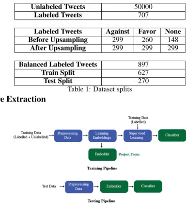
The following table summarizes our dataset. We perform data upsampling to balance our labelled dataset. Since tweets have some unique properties, the preprocessing forms an important step. Specifically, we perform case correction, stop-word/special characters removal, lemmatization, spell check and slang word substitution to clean the data and make it usable. Finally, we split the data 70-30 as train-test.
Unlabeled Tweets 50000
Labeled Tweets 707
Labeled Tweets Against Favor None Before Upsampling 299 260 148
After Upsampling 299 299 299 Balanced Labeled Tweets 897
Train Split 627
Test Split 270
Table 1: Dataset splits
3.2
Feature Extraction
Figure 1:Above: Training Pipeline,Below: Testing Pipeline
Taking inspiration from the prior work, in this project we follow a linear sequential pipeline as depicted in figure 1. Our approach can be bucketed as a heuristic-based semi-supervised learning approach where we explicitly first use the unlabelled data to generate an informed embedding space and then project the labelled data on to this space. The expectation is that, a coherent and informed embedding will allow a classifier to classify data more accurately. At the same time it is important to have these embeddings interpretable so that the approach becomes verifiable and more informative. Exploring how to generate coherent and interpretable embeddings is the core focus of our project. We explore Latent Dirichilet Allocation (LDA) and Para2Vec as our baseline approaches as they are the go-to approaches for generating embeddings in text analytics. We later explore LDA2Vec [14] as the main focus of our project and try to combine the benefits and trade-offs provided by our baselines.
3.3
Supervised Learning
After computing the embedding for our data using feature extraction, we use the labelled data to train a supervised learning based classifier. We use a multi-class SVM classifier for this purpose. To find the best hyper-parameters for the classifier, we do a grid search to select the best parameters
namely the type of kernel to be used and the value of regularization parameter C. After grid search, the classifier with the best 5-fold cross validation accuracy is selected.
4
Embedding Methods
4.1
Topic Modelling: LDA
In order to understand LDA, we first present pLSA (probabilistic Latent Semantic Analysis) [6] that discovers a set of topics related to the collection of documents and its constituent words by factorizing a term-document matrix in a probabilistic manner. Given a documentdin a collection of documents
Di.e.d∈D, a topictis present with probabilityp(t|d). Similarly, given a topictfrom a collection of topicsT i.e.t ∈T, a wordwis present with probabilityp(w|t). We are given a vocabulary of wordsV i.e.w∈V. The joint probability distribution for pLSA can then be expressed as
-P(D, W) =P(W|T)P(T|D)P(D) (1)
Provided the number of topics to be extracted i.e. |T|, we need to find the parameters for the distributionsP(T|D)andP(W|T). These distributions are assumed to be multinomial and modelled using an Expectation-Maximization approach (EM). In the E-step we estimate the distribution
P(t|d, w), while in the maximization step we update our estimates of P(t|d)and P(w|t). The number of parameters is|T||D|+|V||T|. The above process ultimately provides us withP(T|D) i.e. given a document we obtain its topic distribution and use it as a feature representation.
An obvious drawback of pLSA are that we can not assign probabilities to new documents asP(D) is not explicitly modelled. Latent Dirichilet Allocation (LDA)[2] generalizes pLSA by changing the fixed distributionP(D)to a conjucate prior (dirichilet) for the existing multinomial distribution
P(T|D). The parameter that defines this conjucate prior distribution i.e. θis defined by a vector
αwhich is of length|T|. Additionally, a conjucate prior for the existing multinomial distribution
P(W|T)is defined asγand defined by a vectorβof length|W|. To make our life a little easier often the vectorsαandβare assumed to have the same value for all their vector components and reduce to single value parameters. The parametersαandβare treated as hyperparameters and it is an established convention for textual data to set them to50/|T|and0.01respectively [17]. Our final joint probability distribution LDA infers is expressed as
-P(θ, γ, T|W, α, β) (2)
Instead of an EM approach, the most common way of optimizing for the parameters (θ, γ, T) above is through using Gibbs Sampling, a specific form of MCMC (Markov-Chain Monte-Carlo) [5]. Gibbs sampling simulates high-dimensional distribution by sampling on lower-dimensional subsets each independently conditioned on the value of all others. We choose to evaluate LDA as one of our baseline methods and implement it using Mallet [9], a computationally optimized implementation of Gibbs Sampling.
To summarize, LDA will provide us with|T| topics which are each essentially a probability distribution over|W|words. For example if we have 2 topics over 4 words
-t1= [donald: 0.3, trump: 0.6, mexican: 0.1, wall: 0.0] (3)
t2= [donald: 0.0, trump: 0.2, mexican: 0.5, wall: 0.3] (4)
A tweet is then expressed as a probability distribution over these topics which forms our final feature vector representation.
donald trump on the wall= [t1: 0.8, t2: 0.2] (5)
During testing, for a new tweet, each word is assigned a topic distribution using
-P(ti|θ, γ, wj) =P(wj|γ, ti)×P(ti|θ) (6)
whereiis a topic id andjis the word index in the new document. Once we have a per word - topic distribution, we can easily calculate the documents topic distribution by aggregating it.
4.2
Feature Embedding: Para2Vec
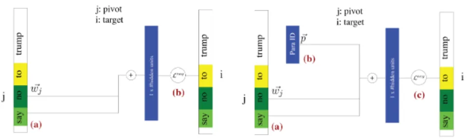
Para2Vec is an interesting addition to the Word2Vec [11] approach which is based on a feed-forward neural network architecture with a single hidden layer. Instead of finding the individual embeddings of each word and averaging them, Para2Vec adds an additional Paragraph vector in the input layer during the training phase that is unique to the paragraph. The training continues as usual, but upon convergence - the paragraph vector holds a numeric representation of the document. This acts as the embedding for a paragraph. In our implementation we use the Gensim library [16] to implement Doc2Vec ( Para2Vec) on our dataset.
Figure 2:Left: Word2Vec Architecture ,Right: Para2Vec Architecture. The colored blocks represent the context window. Green color signifies the pivot words, while yellow signifies the target word in the window.
Both, Word2Vec and Para2Vec approaches are summarized in Figure 2. We use the following notation
-• a document/paragraphdkis a sequence of words{w~k0, ~wk1... ~wkn},w~kj∈Wk∀j ∈[1, n],
where n is the the number of words in the document at indexk.
• a context windowCkis a sequential subset ofdkof size|C|=v. Every word in the context
window is a pivot wordw~kj(j∈[1, v−1]) besides one which is a target word indexed byi
and denoted asw~ik. This context window slides across a document with a fixed stridesin
each iteration.
• each wordw~ is represented as a one-hot vector over the entire vocabulary of the complete corpus i.ew~ ∈R|W|.
• a paragraph vector is also a one-hot vector i.e.d∈R|corpus|.
• the number of hidden units in the only hidden layerhis|h|. We can hence name the matrix between the input layer and the hidden layer asM1∈R|W|×|h|and the matrix between the hidden layer and the output layer asM2∈R|h|×|W|.
In Word2Vec, for a given context windowCkwe compute the values in the hidden layer as
-~h= 1
v−1
X
j∈C,j6=i
M1w~kj (7)
The values in the output layer are modelled as a probability distribution by passing them through a softmax layer
-~o=~hM2 (8)
where~o∈R|W|ando~
frepresents thefthscalar element of the vector.
P(~of|Ck) =
exp(~of)
P
e∈1,..,|W|exp(~oe)
(9)
The loss function is computed as the cross-entropy loss, whereiis the index of the target word.
loss=− X f∈1,..,|W| ~ wkflog exp(~of) P e∈1,..,|W|exp(~oe) (10)
loss=−logP exp(~oi) e∈1,..,|W|exp(~oe) (11) loss=−~oi+ log X e∈1,..,|W| exp(~oe) (12)
A problem with this loss is that computing the gradient computation and update for a large vocabulary size is computationally expensive. To deal with this issue instead of computing the loss for all the non-target words, we do so only for a subsetN. This is known as the negative sampling loss and makes Word2Vec learning more scalable.
loss=−~oi+ log X
e∈N
exp(~oe) (13)
As we can observe in Figure 2, the subtle change made to change Word2Vec into Para2Vec is the inclusion of a document vector to the input nodes. In the abstract sense there is no difference between a word vector and a document vector. A document vectorpadds another matrix that is learned at the end of the trainingM3∈R|Corpus|×|h|. At the time of training the algorithm considers the pivot and the target pairs as the context in Word2Vec, while in Para2Vec the algorithm considers the pivot, target and document triples as the context.
In para2vec the document embeddings are obtained as the rows of theM3 matrix. For a new document obtained during the time of testing, we just retrain the model with the words present in the new document by keepingM1andM2matrices frozen. The embedding obtained is a h-dimensional vector. While the embeddings generated by these couple of methods reflect meaningful properties as a collection, individually the vector generated is not interpretable. As an example, a Para2Vec embedding of the toy tweet mentioned in the previous section would be something like
-donald trump on the wall= [−0.4,0.5, ...5,4] (14)
4.3
LDA2Vec - A Hybrid Approach
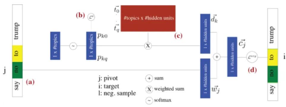
Figure 3: LDA2Vec Architecture
Looking back at the baseline methods we see that Word2Vec is capable at local assessment i.e. given a word it can predict it’s neighbours. Para2Vec adds a global context to this inference and is able to capture both the local sequential context among words and their global relationship in a single embedding. LDA too captures a global context but loses out the sequential nature of the words. This maybe a reason that leads to Para2Vec giving better embeddings. But since LDA provides us with interpretable embeddings (distribution over topics which are essential a ranking of words) it has its own benefits. Taking motivation from the baseline approaches, in this project we explore if we can get both accuracy and interpretability in our feature embeddings. For this we explore LDA2Vec [14], a hybrid approach largely based off of the previously described Para2Vec architecture. The algorithm can be summarized as follows by referencing the annotated components in figure 3
-1. (a)A sliding window runs across the input text belonging to documentk(k∈[1,|corpus|]) and a pivot word is selected, indexed by j in this case, and passed to a linear layer of hidden units. The output of the layer is the|h|dimensional word vectorwkj. We use the same
convention of a context windowCkexplained in the previous section.
2. (b)The number of topics is denoted byq. A q-dimensional document weight vector is randomly initialized and converted to a probability distribution by passing it through a softmax function. For a documentdk we essentially get a q-dimensional vector of the form
[pk1...pkq]
3. Inspired by LDA, the vector is sparsified by using a dirichilet loss function as mentioned below. The strength of this component is controlled by a tuning parameterλ. The sparsity of the vector is controlled byα(more sparse forα <1).
Ldirk =λ q X
x=1
(α−1) logpkx (15)
4. (c)A topic matrixT ∈Rq×|h|is initialized with Vanilla LDA and a document vector(dk) is
created using a weighted sum of the|h|dimensional topic vectorst~0...~tqwhich form the
rows of our topic matrix.
~
dk=pk1.~t1+...+pkq.~tq,0≤pkq ≤1 (16)
5. (d)A context vector is created by taking the sum of the word vector and the document vector.
~
cj=w~kj+d~k (17)
6. The final loss function is a negative sampling loss function (same as equation 13) as described below where l is the index of a fixed number of random negative samples used.
Lnegij = logσ(~cj, ~wi) + X l∈N logσ(−~cj, ~wl) (18) loss=Ldir k + X ij Lnegij (19)
After training the model is able to generate document vectors for each tweet in the datasetd~k. The
special thing about this representation is that it is a weighted sum of the topic vectors[t~1..~tq]where
each topic vector is embedded in the same space as each word in the corpus. Thus, to obtain the words that constitute a topic, we can simply calculates its nearest word neighbours in the embedded space.
5
Results and Analysis
5.1
Using Unlabelled Data
From the evaluation of our baseline methods done prior to the mid-semester checkpoint we drew some interesting conclusions
-1. Table 2 shows the hyper-parameters for LDA, Para2Vec and SVM (with and without unlabelled data) that were learnt through grid-search
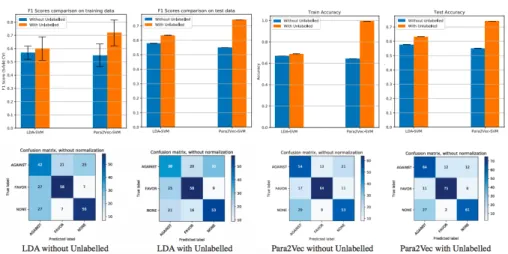
2. One of the most important insights was that using the unlabelled data actually did improve both our baseline methods. This is evident in the accuracy plots and confusion matrices of figure 4 and also on seeing the ROC curve in figure 5.
3. In the same graphs, we also observe that Para2Vec consistently performs better than LDA. On visualizing the T-SNE plots for both the embeddings in figure 5, we can observe that the para2vec embedding is much more structured and uniform as compared to LDA. Although we cannot make any conclusive remarks from the plots, we can observe a small concentration of "NONE" more prominent in the Para2Vec embedding.
4. We also observe that although the embeddings created by Para2Vec seem more coherent than the ones created by LDA (as they lead to a better accuracy on our test set), it is much more difficult to make sense of individual embedding. LDA, although has a lower accuracy, an individual embedding is interpretable as it represents a probability distribution over topics which are themselves a collection of words.
Figure 4: Comparison of training/test F1 scores and training/test accuracy (top) and confusion matrices (bottom)
(a) LDA (44 Topics) (b) Para2Vec (100d) (c) ROC Curve
Figure 5: (a), (b) Comparison of T-SNE representations of labelled data using the two representations. (c) ROC Curve for SVM With and Without Unlabelled Data.
LDA SVM
With Unlabelled |T|= 44 C= 1000,kernel=linear
Without Unlabelled |T|= 44 C= 1000,kernel=linear
Para2Vec SVM
With Unlabelled |h|= 50 C= 1000,kernel=RBF
Without Unlabelled |h|= 50 C= 1000,kernel=linear
Table 2: Tuned hyper-parameters for LDA, Para2Vec and SVM
5.2
LDA2Vec
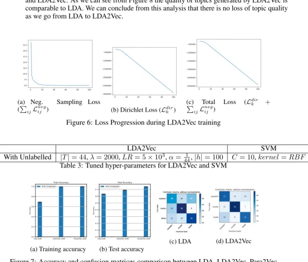
After implementing the hybrid LDA2Vec approach we could draw the following observations : 1. Figure 6 shows loss progression while training our LDA2Vec model on PyTorch. We train
for 100 epochs with a 1024 documents in each batch and as we can see the losses decrease progressively with training. The negative sampling loss falls more steeply while Dirichlet loss falls more linearly.
2. Table 3 shows the parameters that we tuned for LDA2Vec. It also shows hyper-parameters for the best SVM classifier found using grid search.
3. Figure 7 shows accuracy comparison between LDA, LDA2Vec and Para2Vec. As expected we are able to get higher accuracy as compared to LDA (approximately +5% gain) but accuracies are lower as compared to Para2Vec (approximately -8% loss)
4. We do a qualitative analysis between 3 topics and their top 10 words generated by LDA and LDA2Vec. As we can see from Figure 8 the quality of topics generated by LDA2Vec is comparable to LDA. We can conclude from this analysis that there is no loss of topic quality as we go from LDA to LDA2Vec.
(a) Neg. Sampling Loss (P
ijL neg
ij ) (b) Dirichlet Loss (Ldirk )
(c) Total Loss (Ldir
k +
P
ijL neg ij )
Figure 6: Loss Progression during LDA2Vec training
LDA2Vec SVM
With Unlabelled |T|= 44,λ= 2000,LR= 5×10³,α= 1
44,|h|= 100 C= 10,kernel=RBF Table 3: Tuned hyper-parameters for LDA2Vec and SVM
LDA-SVM LDA2Vec-SVM Para2Vec-SVM 0.0 0.2 0.4 0.6 0.8 1.0 A cc ur ac y Train Accuracy With Unlabelled
(a) Training accuracy
LDA-SVM LDA2Vec-SVM Para2Vec-SVM 0.0 0.1 0.2 0.3 0.4 0.5 0.6 0.7 A cc ur ac y Test Accuracy With Unlabelled (b) Test accuracy (c) LDA (d) LDA2Vec
Figure 7: Accuracy and confusion matrices comparison between LDA, LDA2Vec, Para2Vec
Figure 8: Topic comparison between LDA (Left) and LDA2Vec (Right)
5.3
Discussion
From the results above we can see that LDA2Vec proves to be a good middle ground algorithm between LDA and Para2Vec. As we make this claim, we make sure our experiments have remained free from the biases taught to us in the last few classes. We choose the best implementation of LDA and Para2Vec around and perform a thorough grid search to get their best parameters thereby avoiding theTuning Until Bestbias. Since we do not impose any specific constraints to our problem, we consciously try to avoid the confirmation bias by reporting the results as is and incorporating appropriate error bounds in the training plots.
References
[1] Isabelle Augenstein, Andreas Vlachos, and Kalina Bontcheva. USFD at SemEval-2016 Task 6: Any-Target Stance Detection on Twitter with Autoencoders. Technical report.
[2] David M Blei, Andrew Y Ng, and Michael I Jordan. Latent dirichlet allocation. Journal of
machine Learning research, 3(Jan):993–1022, 2003.
[3] Marcelo Dias and Karin Becker. INF-UFRGS-OPINION-MINING at SemEval-2016 Task 6: Automatic Generation of a Training Corpus for Unsupervised Identification of Stance in Tweets. Technical report.
[4] Heba Elfardy and Mona Diab. CU-GWU Perspective at SemEval-2016 Task 6: Ideological Stance Detection in Informal Text. Technical report.
[5] Walter R Gilks, Sylvia Richardson, and David J Spiegelhalter. Introducing markov chain monte carlo.Markov chain Monte Carlo in practice, 1:19, 1996.
[6] Thomas Hofmann. Unsupervised learning by probabilistic latent semantic analysis.Machine learning, 42(1-2):177–196, 2001.
[7] Peter Krejzl and Josef Steinberger. UWB at SemEval-2016 Task 6: Stance Detection. Technical report.
[8] Can Liu, Wen Li, Bradford Demarest, Yue Chen, Sara Couture, Daniel Dakota, Nikita Haduong, Noah Kaufman, Andrew Lamont, Manan Pancholi, Kenneth Steimel, and Sandra K Ubler. IUCL at SemEval-2016 Task 6: An Ensemble Model for Stance Detection in Twitter. Technical report.
[9] Andrew Kachites McCallum. Mallet: A machine learning for language toolkit. 2002.
[10] Tomas Mikolov, Kai Chen, Greg Corrado, and Jeffrey Dean. Efficient estimation of word representations in vector space. CoRR, abs/1301.3781, 2013.
[11] Tomas Mikolov, Ilya Sutskever, Kai Chen, Greg S Corrado, and Jeff Dean. Distributed repre-sentations of words and phrases and their compositionality. InAdvances in neural information
processing systems, pages 3111–3119, 2013.
[12] Amita Misra, Brian Ecker, Theodore Handleman, Nicolas Hahn, and Marilyn Walker. NLDS-UCSC at SemEval-2016 Task 6: A Semi-Supervised Approach to Detecting Stance in Tweets. Technical report.
[13] Saif M. Mohammad, Svetlana Kiritchenko, Parinaz Sobhani, Xiaodan Zhu, and Colin Cherry. Semeval-2016 task 6: Detecting stance in tweets. InProceedings of the International Workshop on Semantic Evaluation, SemEval ’16, San Diego, California, June 2016.
[14] Christopher E Moody. Mixing dirichlet topic models and word embeddings to make lda2vec.
arXiv preprint arXiv:1605.02019, 2016.
[15] Braja Gopal Patra, Dipankar Das, and Sivaji Bandyopadhyay. JU NLP at SemEval-2016 Task 6: Detecting Stance in Tweets using Support Vector Machines. Technical report.
[16] Radim Rehurek and Petr Sojka. Software framework for topic modelling with large corpora. In
In Proceedings of the LREC 2010 Workshop on New Challenges for NLP Frameworks. Citeseer,
2010.
[17] Mark Steyvers and Tom Griffiths. Probabilistic topic models. Handbook of latent semantic analysis, 427(7):424–440.
[18] Martin Tutek, Ivan Sekuli, Paula Gombar, Ivan Paljak, Filip Boltuži, Mladen Karan, Domagoj Alagi, and Jaˇn Snajder. TakeLab at SemEval-2016 Task 6: Stance Classification in Tweets Using a Genetic Algorithm Based Ensemble. Technical report.
[19] Prashanth Vijayaraghavan, Ivan Sysoev, Soroush Vosoughi, and Deb Roy. DeepStance at SemEval-2016 Task 6: Detecting Stance in Tweets Using Character and Word-Level CNNs. Technical report.
[20] Wan Wei, Xiao Zhang, Xuqin Liu, Wei Chen, and Tengjiao Wang. A Specific Convolutional Neural Network System for Effective Stance Detection. Technical Report 6.
[21] Wikipedia contributors. N-gram — Wikipedia, the free encyclopedia. https://en. wikipedia.org/w/index.php?title=N-gram&oldid=885279096, 2019. [Online; ac-cessed 7-March-2019].
[22] Guido Zarrella and Amy Marsh. MITRE at SemEval-2016 Task 6: Transfer Learning for Stance Detection. Technical report.