Relative error accurate statistic based on nonparametric
likelihood
∗Lorenzo Camponovo†
Department of Business Economics, Health and Social Care University of Applied Sciences and Arts of Italian Switzerland
Yukitoshi Matsushita‡ Faculty of Economics Hitotsubashi University
Taisuke Otsu§ Department of Economics London School of Economics October 28, 2020
Abstract
This paper develops a new test statistic for parameters defined by moment conditions that exhibits desirable relative error properties for the approximation of tail area probabilities. Our statistic, called the tilted exponential tilting (TET) statistic, is constructed by estimat-ing certain cumulant generatestimat-ing functions under exponential tiltestimat-ing weights. We show that the asymptoticp-value of the TET statistic can provide an accurate approximation to thep -value of an infeasible saddlepoint statistic, which admits a Lugannani–Rice style adjustment with relative errors of ordern−1 both in normal and large deviation regions. Numerical re-sults illustrate the accuracy of the proposed TET statistic. Our rere-sults cover both just- and over-identified moment condition models. A limitation of our analysis is that the theoretical approximation results are exclusively for the infeasible saddlepoint statistic, and closeness of the p-values for the infeasible statistic to the ones for the feasible TET statistic is only numerically assessed.
∗
The authors are grateful for helpful discussions with Elvezio Ronchetti and Richard Spady and comments by seminar participants at the University of Geneva. The authors also acknowledge helpful comments from the Editor, a Co-Editor, and anonymous referees. Financial supports from the JSPS KAKENHI (18K01541) (Matsushita) and the ERC Consolidator Grant (SNP 615882) (Otsu) are gratefully acknowledged.
†
E-mail: [email protected]. Address: University of Applied Sciences and Arts of Italian Switzer-land, Galleria 2 - 100 Via Cantonale 6928, Manno, CH.
‡
E-mail: [email protected]. Address: Graduate School of Economics, Hitotsubashi University, 2-1 Naka, Kunitachi, Tokyo 186-8601, Japan.
§E-mail: [email protected]. Address: Department of Economics, London School of Economics, Houghton Street, London, WC2A 2AE, UK.
1
Introduction
This paper is concerned with inference on moment condition models and proposes a new test statistic that shows desirable tail behaviors in terms of relative errors. For this problem, there are various test statistics available in the literature, such as the Wald, empirical likelihood (Owen, 1988), exponential tilting (Efron, 1981, 1982, Kitamura and Stutzer, 1997, and Imbens, Spady and Johnson, 1998), power divergence (Baggerly, 1998), and saddlepoint statistics (Robinson, Ronchetti and Young, 2003, and Ma and Ronchetti, 2011), among others. In particular, it is known that the empirical likelihood statistic admits the Bartlett correction, a higher-order refinement for the absolute error of the type I error probability (DiCiccio, Hall and Romano, 1991). This refinement in the absolute error is typically not achieved by other statistics, such as exponential tilting (Jing and Wood, 1996, and Baggerly, 1998).
For statistical inference, researchers are commonly interested in the accuracy of approxima-tions for tail area probabilities or p-values of test statistics. For this purpose, the relative error rather than the absolute one delivers a more relevant measure of accuracy, and various procedures typically based on saddlepoint approximations are developed (Tingley and Field, 1990, Daniels and Young, 1991, Jing and Robinson, 1994, Robinson, Ronchetti and Young, 2003, and Kolassa and Robinson, 2011, among others). In particular, Robinson, Ronchetti and Young (2003) con-sidered the situation where the cumulant generating function is known to the researcher and developed a novel saddlepoint statistic that is asymptotically chi-squared distributed with a rel-ative error of order n−1 even in the large deviation region. Although this statistic is generally infeasible due to the requirement on the knowledge of the cumulant generating function, Robin-son, Ronchetti and Young (2003) and Ma and Ronchetti (2011) proposed some feasible versions of the saddlepoint statistic by using the exponential tilting weights (Efron, 1981, 1982).
The basic idea of our statistic is to note that the conventional exponential tilting statistic is constructed from estimating the cumulant generating function by the sample average, and to modify the cumulant estimation by using the exponential tilting weights instead of the uniform weights. In other words, we tilt the exponential tilting statistic. Thus, the new statistic is called the tilted exponential tilting (TET) statistic.
We show that the TET statistic is asymptotically chi-squared distributed, and demonstrate that its asymptotic p-value provides an accurate approximation to the p-value of some ideal (but infeasible) saddlepoint statistic, which admits a Lugannani–Rice style adjustment with a relative error of order n−1 both in normal and large deviation regions. Thus, as far as the
argue that the asymptotic p-value approximation for the TET statistic using the chi-squared distribution is very accurate even in the tails. Due to technical difficulty, however, this paper only establishes the theoretical approximation results for the ideal saddlepoint statistic, and admittedly the approximation property between the ideal saddlepoint and feasible TET statistics is only numerically investigated. We note that both the TET and ideal statistics are new in the literature, and different from the saddlepoint statistics discussed above. Furthermore, our results on the TET statistic cover both just- and over-identified moment condition models.
We emphasize that accuracy ofp-values in tail areas for testing moment condition models is a substantial issue in applied research. In practice, researchers are concerned with accuracy of relatively smallp-values (say, less than 10%) which will be typical borderlines to decide whether the null should be rejected or not. As our simulation studies below indicate, the empirical quantiles of the TET statistic are very close to the ones of the limiting chi-squared distribution for the tail areas. Furthermore, we note that moment condition models are widely used in empirical economic analyses, and it is well known that the (first-order) asymptotic approximations for those models may not provide accurate inference methods in small to moderate samples (see, e.g., the special issue in the Journal of Business & Economic Statistics, vol. 14).
Finally, we study through Monte Carlo simulations the accuracy of the proposed TET statis-tic. In addition to a benchmark setup for inference on means, we consider both just- and over-identified instrumental variable regression models. The numerical results highlight a desir-able accuracy of our test statistic. In particular, the empirical quantiles of the TET statistic are extremely close to those of the limiting distribution even for small sample sizes.
This paper is organized as follows. In Section 2, we consider a benchmark case, simple parameter hypothesis testing for just-identified moment conditions, and present basic theoretical results illustrated by a small simulation study. Section 3 extends our method to testing problems for composite hypotheses (Section 3.1), and overidentifying restrictions (Section 3.2). Finally, Section 4 presents simulation results for the general case. All proofs are presented in Appendix A. Appendix B contains figures for simulation results in Section 4.
2
Benchmark case
In this section, we present the basic idea of the new test statistic and its theoretical and numerical properties under a benchmark setup. Section 2.1 introduces our TET statistic. Section 2.2 illustrates its finite sample accuracy through Monte Carlo simulation. In Section 2.3, we discuss that the TET statistic has desirable relative error properties for the approximation of tail area
probabilities.
2.1 Tilted exponential tilting statistic
Suppose we observe an i.i.d. sample {Xi}ni=1 of X. Let F be the distribution function ofX and
E[·]be the expectation underF. Consider the (just-identified) moment conditions
E[g(X, θ0)] = 0,
where g is ap-dimensional vector of moment functions and θ0 is ap-dimensional vector of true
parameter values. In this section, we focus on hypothesis testing for the null H0 :θ0= 0 against
the two-sided alternative H1 :θ0 6= 0. Since we do not specify the parametric distribution form
of X, testing methods based on parametric likelihood theory, such as the likelihood ratio and score tests, are not applicable. However, there are several ways to test H0 in this setting. For
example, we can implement the Wald test based on some estimator of θ0. Also based on some
nonparametric likelihood, we can conduct likelihood ratio or score type tests (see, e.g., Owen, 2001).
We propose a new test statistic for H0, which exhibits a desirable finite sample accuracy.
Our test statistic is constructed by evaluating the exponential tilting statistic (Efron, 1981, 1982, Kitamura and Stutzer, 1997, and Imbens, Spady and Johnson, 1998) under the exponential tilting weights based on the restriction E[g(X, θ0)] = 0 under the nullH0 :θ0= 0. Letλˆ be a solution
of Pn
i=1e ˆ
λ0g(Xi,0)g(X
i,0) = 0. The conventional exponential tilting statistic for H0 :θ0 = 0 is
written as Tnet=−2 log 1 n n X i=1 eλˆ0g(Xi,0) ! . (1)
It is known that nTnet converges in distribution to the χ2p distribution under H0. This statistic
is obtained by minimization of the empirical relative entropy
min π1,...,πn n X i=1 nπilog(nπi), s.t. n X i=1 πig(Xi,0) = 0, n X i=1 πi = 1.
By applying the Lagrange multiplier method, the solution is written as
ˆ πi = eλˆ0g(Xi,0) Pn j=1e ˆ λ0g(X j,0) ,
fori= 1, . . . , n. Note that by construction these optimal weights are positive and satisfy the mo-ment conditionPn
is an asymptotically efficient estimator of the distribution function of X under the restriction
E[g(X, θ0)] = 0 subject to the nullH0 :θ0 = 0 (Brown and Newey, 1998).
Intuitively, the exponential tilting statisticTnetis constructed by taking expectation ofeˆλ0g(Xi,0)
under the empirical distribution with weights1/n. Our proposal is to replace the uniform weights by the optimal ones under H0, and to take expectation of eλˆ
0g(X
i,0) under the tilted empirical
distribution with weights {πˆi}ni=1, that is
Tntet= 2 log n X i=1 ˆ πie ˆ λ0g(Xi,0) ! = 2 " log n X i=1 e2ˆλ0g(Xi,0) ! −log n X i=1 eλˆ0g(Xi,0) !# . (2)
We call this statistic the tilted exponential tilting (TET) statistic. As shown in the proof of Theorem 1, the reason for the positive sign of Tntet can be seen from a second-order expansion aroundλˆ0g(Xi,0) = 0, nTntet=nλˆ0 " n X i=1 ˆ πig(Xi,0)g(Xi,0)0 # ˆ λ+op(1),
underH0, where we usedPni=1πˆig(Xi,0) = 0. It will be shown that the right hand side converges
in distribution to the χ2p distribution under H0. To make the argument rigorous, we impose the
following assumption.
Assumption 1. {Xi}ni=1 is i.i.d., E[|g(X, θ0)|ζ]<∞ for some ζ > 2, and E[g(X, θ0)g(X, θ0)0]
is nonsingular.
All conditions are standard. Based on these conditions, the limiting null distribution of the TET statistic is obtained as follows.
Theorem 1. Under Assumption 1 and H0 : θ0 = 0, the TET statistic nTntet converges in
distribution to the χ2p distribution.
Therefore, underH0, the TET statisticnTntetis asymptotically equivalent to the exponential
tilting statisticnTnet. We can also show that they have the same local power function under local alternatives.
2.2 Simulation for benchmark case
To illustrate finite sample accuracy of the TET statistic, we provide a preliminary simulation result. We generate random samples {Xi}ni=1 of sizes n = 20, 40, and 80 according to Xi ∼
We are interested in testing the null hypothesis H0 :θ0 = 0against the alternative H1:θ0 6= 0,
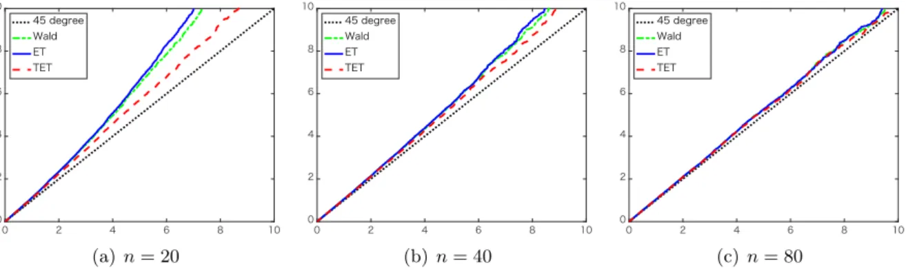
and compare the proposed TET statistic nTntet with the exponential tilting statistic nTnet and the conventional Wald statistic. All the statistics converge in distribution to the χ21 distribution underH0. Figure 1 reports the q-q plots of the empirical quantiles of these test statistics against
those of theχ21 distribution. The number of Monte Carlo replications is 20,000.
(a)n= 20 (b) n= 40 (c) n= 80
Figure 1: Empirical quantiles of the TET statistic (dashed red line), exponential tilting statistic (solid blue line), and Wald statistic (dash-dotted green line) against quantiles of the χ21 distri-bution for (a) n= 20, (b)n= 40, and (c) n= 80.
As this figure shows, the empirical quantiles of the TET statistic are closer to those of the limiting χ21 distribution even for relatively small sample sizes. The accuracies of the exponential tilting and Wald statistics increase as the sample size increases, although the TET statistic outperforms for all cases. In the next subsection, we provide some explanation for this excellent finite sample performance of the TET statistic.
2.3 Relative error properties
2.3.1 Overview
The main purpose of this paper is to provide some theoretical justification for the desirable accuracy of the TET statistic nTntet using χ2 asymptotic approximation particularly in the tail area as observed in the q-q plots in the last subsection. Based on the statistics literature of saddlepoint approximations (see, e.g., Jensen, 1995, for a review), an ideal goal for this purpose is to evaluate the order (say,%n) in the relative error for the χ2 asymptotic approximation:
Pr{nTntet≥nt:F}={1−Fp(nt)}(1 +O(%n)), (3)
and compare the approximation error O(%n) with the ones for other statistics, where Fp is
saddlepoint approximations are mostly confined to smooth function models for finite dimensional sample means and parametric models, and it is difficult to establish the approximation result for the TET statistic as in (3) under moment condition models. To the best of our knowledge, there is no relative error approximation results for the GMM or generalized empirical likelihood-based statistic under general moment condition models.
To circumvent this technical difficulty, we consider an infeasible version of the TET statistic, calledTnin (5) below, by replacing the weighted average in (2) using{πˆi}ni=1with the population
mean. Although Tn is infeasible, it is possible to establish certain relative error approximation
results for Pr{nTn≥nt:F} as in (3) (see, Theorem 2 below).
Based on these considerations, we assume that the p-value ptet = Pr{nTntet ≥ nttet,o : F} for the TET statistic is well approximated by its infeasible version pideal = Pr{nT
n ≥nto :F},
wherettet,o andtoare observed values ofTntetandTn, respectively. Then, under this assumption,
we concentrate on the relative error properties to approximate the p-value of the proxypideal for
ptet. Our main results (Theorems 2 and 3 below) establish the relation between pideal and the asymptotic p-value pasy= 1−F
p(nttet,o) for our TET test as
pideal=pasy(1 +rn(ˆλo))(1 +O(n−1)), (4)
where λˆo is an observed value of ˆλ and rn(·) is a function defined in (19). Based on this
relative error approximation, we argue thatrn(·)exhibits a desirable property not shared by the
conventional exponential tilting test.
A major limitation of this paper is that due to technical difficulty in analyzing Tntet, we cannot provide any theory to characterize the quality of the approximation forptetbypideal. The original object of interest, the ratio of the p-value ptet of the TET statistic to its asymptotic approximation pasy, can be decomposed as
ptet
pasy = (1 +ρ1)(1 +ρ2),
whereρ1 = (ptet−pideal)/pideal andρ2= (pideal−pasy)/pasy. Our result in (4) only characterizes
ρ2. For the benchmark simulation in Section 2.2, we evaluate the magnitudes of the component
ρ1 by the ratios ρ1 ρ2
for 1000 Monte Carlo replications, and find that their interquartile ranges
are: [0.49,1.71]for n= 20,[0.53,1.47]for n= 40, and [0.57,1.45]for n= 80. Thus, at least for the benchmark simulation setup, the approximation error ρ1 is comparable to ρ2, which will be
be left for future research.
2.3.2 Ideal statistic Tn
We now introduce the ideal statistic Tn. In the definition of the TET statistic (2), we propose
to take expectation of eˆλ0g(Xi,0) under the tilted weights {πˆ
i}ni=1 satisfying Pn
i=1πˆig(Xi,0) = 0.
The ideal (but infeasible) statistic is given by evaluating this expectation under the population:
Tn= 2K(ˆλ), (5)
where K(λ) = logE[eλ
0g(X,0)
] is the cumulant generating function of g(X,0), and λˆ solves
Pn
i=1e ˆ
λ0g(Xi,0)g(X
i,0) = 0. Observe that Tn is infeasible because it involves the expectation
E[·] to evaluate the cumulant. Furthermore, Tn is different from the saddlepoint statistic
pro-posed in Robinson, Ronchetti and Young (2003) because it does not involve any estimators of
θ0.
To study the relative error property of Tn, we introduce further notation. Let gˇ(x) =
E[g(X,0)g(X,0)0]−1/2g(x,0) be a normalized counterpart of g(x,0) so that V ar(ˇg(X)) = I,
and define ˇλ= E[g(X,0)g(X,0)0]1/2λˆ. Based on the definition of λˆ, λˇ can be written as a
so-lution of Pn
i=1ψ(Xi,λˇ) = 0, where ψ(x, y) = −ey
0gˇ(x) ˇ
g(x). Thus, ψ(x, y) may be interpreted as an estimating function for λˇ. Also let K(t, y) = logE[et
0ψ(X,y)
] and t(y) be a solution of
∂K(t(y),y)
∂t = 0. We impose the following high level assumption.
Assumption 2. The density fˇλ of ˇλexists and has the saddlepoint approximation
fˇλ(y) = n 2π p/2 e−nh(y)pdetB(y) det Σ(y)(1 +O(n −1)), (6) where h(y) = K(t(y), y), B(y) = enK(t(y),y)E et(y)0ψ(X,y)∂ψ(X, y) ∂y , Σ(y) = enK(t(y),y)E[et(y) 0ψ(X,y) ψ(X, y)ψ(X, y)0].
Assumption 2 requires existence of the usual form of the saddlepoint approximation of the density of ˇλ. We note that the saddlepoint approximation error in (6) is typically of relative order O(n−1). For primitive conditions under which this assumption holds, we refer to Field (1982), Skovgaard (1990), Jensen and Wood (1998), and Almudevar, Field and Robinson (2000).
For example, suppose E[g(X,0)g(X,0)0] is invertible and all components in ψ(x, y) and their
first four derivatives with respect to y are bounded and continuous as functions ofx at each y. Then certain smoothness conditions that enable the development of an Edgeworth expansion are sufficient to guarantee Assumption 2 (see, Ma and Ronchetti, 2011, pp. 154-155).1,2
Let Fp be the cumulative distribution function of the χ2p distribution. The relative error
property for the approximation of the tail area probability of Tn is established as follows.
Theorem 2. Suppose that Assumptions 1 and 2 hold. Then underH0 :θ0 = 0,
Pr{nTn≥nt:F}={1−Fp(nξ(t))}(1 +O(n−1)), (7)
uniformly over t∈ (0, ε) for some ε >0, where ξ(t) = √t−logG(
√ t) n√t 2 and G(·) is defined in (17) in the Appendix.
Theorem 2 provides a Lugannani–Rice style accurate approximation formula for the tail area probability of Tn. This approximation holds not only for the normal region (i.e., nt is
bounded) but also for the large deviation region (i.e., t is bounded). This theorem shows that the ideal statistic Tn admits a relative error of order O(n−1) up to the large deviation region.
Note that relative error orders typically deliver a more useful measure of the quality of tail area approximation compared to absolute ones. Robinson, Ronchetti and Young (2003) established an analogous desirable relative error property for their saddlepoint statistic, which is also infeasible in the present setup. Also, Huber and Ronchetti (2009, ch. 14.6) argued that for parametric models the three classical hypothesis tests (i.e., likelihood ratio, Wald, and score) do not satisfy the relative error property as in (7).
1
More precisely, letUy = (U1y0, U
y0 2 , U y0 2 ), whereU y 1 = ψ(X, y), U y
2 is the vector formed by the elements of
∂ψ(X, y)/∂y0 andψ(X, y)ψ(X, y)0, andU3yis the vector formed by the elements of∂U2y/∂y0. Then letFUy be the distribution function ofUy and define a random vectorU˜ywith the distribution function
FU˜y(u1, u2, u3) =
ˆ
(a1,a2,a3)≤(u1,u2,u3)
et(y)0a1−K(t(y),y)dFy
U(a1, a2, a3),
and the characteristic functionφy(ξ) =E[eiξ 0U˜y
]. Based on this notation, the smoothness condition is stated as: for eachy, there exist positive constantsc,C, andc1such that (i)c <det(V ar( ˜Uy))< C, and (ii)|φy(ξ)| ≤1−c1
for allc <|ξ|< Cn(dim ˜Uy+1)/2.
2To be specific, consider the (just-identified) instrumental variable regression model, whereg(X, Y, Z, θ
0) =
Z(Y −X0θ0)for a dependent variableY, endogenous regressorsX, and instrumental variablesZ. Assumptions
1 and 2 are satisfied if{Xi, Yi, Zi}ni=1is i.i.d.,E[g(X, Y, Z, θ0)g(X, Y, Z, θ0)0]invertible, and the random variable
W = g(X, Y, Z, θ0) is continuously distributed on some compact support W, which is typically guaranteed by
the compact support of the observables(Y, X0, Z0). Although this is a rather restrictive sufficient condition, our simulation studies in Sections 2.2 and 4 do not impose compact support for the data and we can still observe desirable performances of the TET statistic.
We note that most existing results using the saddlepoint approximation require finite moment generating functions (around zero) for the estimating equations (i.e.,ψ(X, y)in our notation). A notable exception is Jing, Shao and Zhou (2004) who established the saddlepoint approximation for tail probabilities of the t-statistic with no moment conditions. Although it is beyond the scope of this paper, it is interesting to see whether their theoretical development can be adapted to our context.
The adjustment by the transformξ(t)to achieve relative error refinement is analogous to the one in Kolassa and Robinson (2011) for the (parametric) likelihood ratio statistic. In general, the functionG(·)requires numerical integration over a sphere of dimensionp, but a Monte Carlo approximation to any degree of accuracy required can be obtained; see Kolassa and Robinson (2011) for details.
2.3.3 Relative error property of the TET statistic
Motivated by the desirable relative error property of the ideal statistic Tn, we now establish the
result in (4) and argue that the TET statistic Ttet
n provides an accurate approximation to the
tail area probabilities of the ideal statistic Tn. To this end, we introduce the function
Ktet(λ) = log n X i=1 ˆ πoieλ0g(xoi,0) ! , where {xoi}n
i=1 and {πˆio}ni=1 are the observed values of {Xi}ni=1 and {ˆπi}ni=1, respectively. We
can see that the observed values of Tn and Tntet are given bytn= 2K(ˆλo) and ttetn = 2Ktet(ˆλo),
respectively, whereλˆo is the observed value ofλˆ. Taylor expansions ofK(λ)andKtet(λ)around
λ= 0 yield K(λ) = 1 2λ 0 E[g(X,0)g(X,0)0]λ+O(|λ|3), Ktet(λ) = 1 2λ 0 n X i=1 ˆ πiog(xoi,0)g(xoi,0)0 ! λ+O(|λ|3). (8)
These expansions highlight some interesting analogies between Tn and Tntet. By the argument
in the proof of Theorem 1, the sample counterpart of the difference K(λ)−Ktet(λ) is of order
Op(n−1/2|λ|2).
On the other hand, if we consider an analogous functionKet(λ) =−logn1Pn
i=1eλ 0g(xo
i,0)
for the exponential tilting statistic so that tetn = 2Ket(ˆλo), then an expansion yields
Ket(λ) =−λ0¯go−1 2λ 0ˆ Voλ+O(|λ|3), (9) where ¯go = n1Pn i=1g(xoi,0) and Vˆo = n1 Pn i=1(g(xoi,0)−g¯o)(g(xoi,0)−g¯o)
0. In this case, the
sample counterpart of the difference K(λ)−Ket(λ) is of order O
p(max{n−1/2|λ|,|λ|2}). Also
we can see that the same comment applies to the function Kcu(λ) = −λ0g¯o− 1 2λ
0Vˆoλ for the
continuous updating GMM, i.e., the sample counterpart of the difference K(λ)−Kcu(λ) is of
Wald statistic.3
The following theorem shows thatKtet(λ)can provide an accurate approximation to the tail area probabilities ofTn.
Theorem 3. Suppose that Assumptions 1 and 2 hold true. Then under H0 :θ0= 0, it holds
1−Fp(nξ(K(λ))) ={1−Fp(nKtet(λ))}(1 +rn(λ))(1 +O(n−1)),
for each realization {xoi}n
i=1, where rn(λ) is a nonrandom function of λ defined in (19) and its
sample counterpart, obtained by replacing {xoi}n
i=1 with {Xi}ni=1, is of order Op(n1/2|λ|2).
Theorem 3 shows that the TET statistic can provide an accurate approximation to the tail area probability formula 1−Fp(nξ(K(λ))) for the ideal statistic Tn in (7). The error of this
approximation is relative and of (stochastic) order n1/2|λ|2. Therefore, in the normal region for
λ=O(n−1/2), the relative error is of ordern−1/2. Beyond the normal region, e.g.,λ=O(n−1/3), the relative error approximation is of order n−1/6. On the other hand, it is clear from (9) that the function Ket(λ) for exponential tilting does not have such a relative error property.
Combining Theorems 2 and 3 (evaluated at λ = ˆλo), we can establish the equality in (4). Therefore, as far as the p-valueptetfor the TET statistic is well approximated by the one pideal
for the ideal statisticTn, we can argue that the asymptotic approximation for the TET tends to
be accurate particularly in the tail area as illustrated in Figure 1 for the benchmark simulation.
3
General case
In this section, we generalize the theoretical results obtained in the last section for testing composite hypotheses (Section 3.1) and overidentifying restrictions (Section 3.2).
3.1 Composite hypothesis test
In this subsection, we extend the results for the benchmark case to composite hypothesis testing. We first consider just-identified moment conditions, and then discuss how to adapt our results for overidentified models.
3
Similarly, even if we consider the class of generalized empirical likelihood criterion by Newey and Smith (2004) (i.e., Kgel(λ) = 1
n Pn
i=1ρ(λ
0
g(xoi,0))for a concave function ρ), we can see that the sample counterpart of the difference K(λ)−Kgel(λ) is of order Op(max{n−1/2|λ|,|λ|2}). However, we conjecture that a ‘tilted’ version of the generalized empirical likelihoodKtgel(λ) =Pn
i=1πˆ o
ρ,iρ(λ 0
g(xoi,0))will exhibit a similar property as Ktet(λ)in Theorem 3, whereπˆρ,io =ρ1(ˆλoρ0g(xoi,0))/
Pn i=1ρ1(ˆλ
o0
ρg(xoi,0))is the generalized empirical likelihood implied probability with ρ1(v) =∂ρ(v)/∂vand ˆλoρ= arg maxλPni=1ρ(λ
0
g(xo
i,0)). We note that in contrast to the (observed) TET statisticttetn = 2Ktet(ˆλo), its generalized empirical likelihood counterparttgeln = 2Ktgel(ˆλo) involves two Lagrange multipliers,λˆo
3.1.1 Just-identified case
Consider just-identified moment conditions E[g(X, θ10, θ20)] = 0, whereθ10 and θ20 are p1- and
p2-dimensional parameters, respectively, and g is a p = p1+p2 dimensional vector of moment
functions. Suppose we wish to test the null hypothesis H0 : θ20 = 0 against the two-sided
alternative H1 : θ20 6= 0. In this case, the conventional exponential tilting statistic may be
written as Tn,cet =−2 max θ1∈Θ1 log 1 n n X i=1 eλˆ(θ1)0g(Xi,θ1,0) ! , (10) where λˆ(θ1) solves Pni=1eˆλ(θ1) 0g(X i,θ1,0)g(X
i, θ1,0) = 0 for eachθ1. It is known that nTn,cet
con-verges in distribution to the χ2p2 distribution under H0 : θ20 = 0. Let θ˜1 be a solution of the
above constrained maximization for θ1 and θ˜= (˜θ01,00)0. The TET statistic for the composite
hypothesis is constructed as Tn,ctet= 2 log n X i=1 ˜ πie ˜ λ0g(Xi,θ˜) ! = 2 " log n X i=1 e2˜λ0g(Xi,θ˜) ! −log n X i=1 e˜λ0g(Xi,θ˜) !# , (11) where π˜i = e ˜ λ0g(Xi,θ˜) Pn j=1e ˜ λ0g(Xj ,θ˜) and ˜λ solves Pn i=1e ˜ λ0g(X i,θ˜)g(X
i,θ˜) = 0. Similar to the last section,
we consider the ideal but infeasible statistic
Tn,c= 2K(˜λ,θ˜1(˜λ)), where K(λ, θ1) = logE[eλ 0g(X,θ 1,0)] and θ˜ 1(λ) solves E h eλ0g(X,θ˜1(λ),0)λ0 ∂g(X,θ˜1(λ),0) ∂θ01 i = 0 for each λ. To analyze the relation between the Tn,ctet and Tn,c consider the function Ktet(λ, θ1) = log Pn i=1π˜oieλ 0g(xo i,θ1,0) , where {˜πoi}n
i=1 are the observed values of {π˜i}ni=1. Note that the
ob-served value ofTn,ctetis given byttetn,c= 2Ktet(˜λo,θ˜tet1 (˜λo)), whereλ˜o is the observed value ofλ˜and
˜ θtet1 (λ)solves n1Pn i=1eλ 0g(xo i,θ˜tet1 (λ),0)λ0 ∂g(xo i,θ˜tet1 (λ),0) ∂θ10
= 0 for eachλ. To analyze the properties of the TET statistic Tn,ctet, we modify Assumption 1 as follows.
Assumption 1’. {Xi}ni=1 is i.i.d., θ10 ∈ intΘ1 is the unique solution of E[g(X, θ10, θ20)] = 0, Θ1 is compact, g(x, θ1, θ20) is continuous at each θ1 ∈ Θ1 and is continuously differentiable
in a neighborhood N of θ10 for almost every x, E[supθ1∈Θ1|g(X, θ1, θ20)|
ζ] < ∞ for some
ζ > 2, E[supθ1∈N|∂g(X, θ1, θ20)/∂θ
0
1|] < ∞, E[∂g(X, θ10, θ20)/∂θ10] is full column rank, and
E[g(X, θ0)g(X, θ0)0] is nonsingular.
Theorem 4. Suppose that Assumption 1’ holds true and that Assumption 2 is satisfied with
˜
g(X, θ0) in (21) instead of g(X,0). Then under H0 :θ20= 0,
(i) the ideal statistic Tn,c satisfies
Pr{nTn,c≥nt:F}={1−Fp2(nξc(t))}(1 +O(n
−1)),
uniformly over t ∈ (0, ε) for some ε > 0, where ξc(t) is defined as in ξ(t) (by replacing
g(X,0) with ˜g(X, θ0)),
(ii) Ktet(λ, θ1) satisfies
1−Fp2(nξc(K(λ,θ˜1(λ)))) ={1−Fp2(nK
tet(λ,θ˜tet
1 (λ)))}(1 +rn,c(λ))(1 +O(n−1)),
for each realization {xoi}n
i=1, where rn,c(λ) is a nonrandom function of λ and its sample
counterpart, obtained by replacing {xoi}n
i=1 with {Xi}ni=1, is of order Op(n1/2|λ|2).
Theorem 4 (i) highlights the desirable relative error property of the ideal statisticTn,c.
The-orem 4 (ii) shows that the TET statistic can be expected to provide accurate approximations of the tail area probabilities of the ideal statistic Tn,c.
We can compare with the saddlepoint statistic introduced in Ma and Ronchetti (2011). In this case, their statistic is written as
2 " log n X i=1 e˜λ0g(Xi,θ˜) ! −log n X i=1 e˜λ0g(Xi,θ˜)+ˆµ0g(Xi,θ¯1,θˆ2) !# , where θˆ= (ˆθ10,θˆ20)0 solvesPn i=1g(Xi,θˆ) = 0, µˆ and θ¯1 solve Pn i=1π˜ieµˆ 0g(X i,θ¯1,0)g(X i,θ¯1,θˆ2) = 0 and µˆ0Pn i=1π˜ieµˆ 0g(X i,θˆ)∂g(X
i,θ¯1,θˆ2)/∂θ01 = 0. Note that this saddlepoint statistic requires to
solve several equations to obtain θˆ, θ˜, θ¯1, λ˜, and µˆ. In contrast, the TET statistic nTn,ctet only
requires to solve for θ˜andλ˜.4
4
Although the TET statistic nTn,ctet takes a simpler form than Ma and Ronchetti’s (2011), we still need to compute θ˜= (˜θ10,0
0
)0 and λ˜ to implement our test. The computation of λ˜ (for a given θ) can be formulated˜ as a convex optimization problem so that Newton iterations can be applied. We use the matlab codes provided by Kirill Evdokimov and Yuichi Kitamura (available at https://www.kirillevdokimov.com/EL_codes.zip) for our numerical studies. On the other hand, the computation ofθ˜typically requires a nested optimization algorithm, where the inner loop computesˆλ(θ1)for eachθ1, and the outer loop computesθ˜1 in (10). Similar to˜λ, the inner
loop is typically a convex optimization problem which can be implemented by Newton iterations. The outer loop is a general nonlinear optimization problem, and we employ a quasi-Newton method, which works well in our numerical studies. See Kitamura (2007) for a detailed discussion on the nested optimization algorithm.
3.1.2 Overidentified case
The results in Theorem 4 can be adapted to overidentified models. For overidentified moment conditions E[g(X, θ10, θ20)] = 0, whereθ10 and θ20 are p1- and p2-dimensional, respectively, and
g is d > p1+p2 dimensional, suppose we wish to test the null hypothesis H0 :θ20 = 0 against
the two-sided alternative H1 :θ206= 0. Indeed this testing problem can be written as the one for
H0 :θ20= 0 in the following augmented moment conditions
E[h(X, µ0, θ10, θ20)] =E eµ00g(X,θ10,θ20)g(X, θ 10, θ20) eµ00g(Xi,θ10,θ20) ∂g(X,θ10,θ20) ∂(θ01,θ20) 0 µ0 = 0.
Note that due to the additional d-dimensional parameters µ0, this moment condition model
is just-identified. Therefore, the results in Section 3.1.1 for the just-identified case can be adapted by replacing the moment function g(·) with h(·), and nuisance parameters θ10 with
ϑ10= (θ100 , µ00)0. Letϑ˜1 = arg maxϑ1log
1 n Pn i=1e ˆ λ(ϑ1)0h(Xi,ϑ1,0) , whereλˆ(ϑ1) solves Pn i=1e ˆ λ(ϑ1)0h(Xi,ϑ1,0)h(X
i, ϑ1,0) = 0for each ϑ1. The TET statistic is defined as
Tn,ctet1 = 2 log n X i=1 ˜ πie ˜ λ0h(Xi,ϑ˜) ! , where ϑ˜= ( ˜ϑ01,00)0, ˜πi = e ˜ λ0h(Xi,ϑ˜) Pn j=1e ˜ λ0h(Xj ,ϑ˜), and λ˜ solves Pn i=1e ˜ λ0h(X i,ϑ˜)h(X i,ϑ˜) = 0. By applying
the results in Theorem 4, analogous relative error properties for Tn,ctet1 can be derived.
3.2 Overidentifying restriction test
In this subsection, we consider the case of overidentifying moment restrictions E[g(X, θ0)] = 0, where the dimension d of the moment functions g is larger than the dimension p of the unknown parameters θ0. In particular, we focus on testing overidentifying restrictions, i.e.,
H0 : E[g(X, θ)] = 0 for some θ against H1 : E[g(X, θ)] 6= 0 for any θ. This is a specification
testing problem for the model specified by moment restrictions. In this case, the conventional exponential tilting statistic may be written as
Tn,vet =−2 max θ log 1 n n X i=1 eλˆ(θ)0g(Xi,θ) ! , (12)
where λˆ(θ) is defined in the last subsection. Based on Newey and Smith (2004), we can show that nTn,vet converges in distribution to the χ2d−p distribution under the null hypothesis. Let θ¯
restriction test is constructed as Tn,vtet= 2 log n X i=1 ¯ πie ¯ λ0g(Xi,θ¯) ! = 2 " log n X i=1 e2¯λ0g(Xi,θ¯) ! −log n X i=1 eλ¯0g(Xi,θ¯) !# , (13) where π¯i = e ¯ λ0g(Xi,θ¯) Pn j=1e ¯ λ0g(Xj ,θ¯) and λ¯ solves Pn i=1e ¯ λ0g(Xi,θ¯)g(X
i,θ¯) = 0. In this case, the ideal but
infeasible statistic is defined as
Tn,v = 2K(¯λ,θ¯(λ)). where θ¯(λ) solves E h eλ0g(X,θ¯(λ))λ0 ∂g(X,θ¯(λ)) ∂θ0 i
= 0. Next, consider the function Ktet(λ, θ) = logPn i=1π¯oieλ 0g(xo i,θ) , where{π¯io}n
i=1are the observed values of{π¯i}ni=1. Note that the observed
value ofTn,vtetis given byttetn,v = 2Ktet(¯λo,θ¯tet(¯λo)), whereλ¯ois the observed value ofλ¯andθ¯tet(λ)
solves 1nPn i=1eλ 0g(xo i,θ¯tet(λ))λ0 ∂g(xo i,θ¯tet(λ)) ∂θ0
= 0for eachλ. To analyze the properties of the TET statistic Tn,vtet, we modify Assumption 1 as follows.
Assumption 1”. {Xi}ni=1 is i.i.d., θ0 ∈ intΘ is the unique solution of E[g(X, θ0)] = 0, Θ is
compact, g(x, θ) is continuous at eachθ∈Θand is continuously differentiable in a neighborhood N ofθ0 for almost everyx,E[supθ∈Θ|g(X, θ)|ζ]<∞for someζ >2,E[supθ∈N |∂g(X, θ)/∂θ0|]<
∞,E[∂g(X, θ0)/∂θ0]is full column rank, and E[g(X, θ0)g(X, θ0)0] is nonsingular.
The relative error properties ofTn,v and Tn,vtet are presented as follows.
Theorem 5. Suppose that Assumption 1” holds true and the adapted version of Assumption 2
is satisfied. Then under H0 :E[g(X, θ0)] = 0,
(i) the ideal statistic Tn,v satisfies
Pr{nTn,v ≥nt:F}={1−Fd−p(nξv(t))}(1 +O(n−1)),
uniformly over t∈(0, ε) for someε >0, whereξv(t) is defined as in ξ(t),
(ii) Ktet(λ, θ) satisfies
1−Fd−p(nξv(K(λ,θ¯(λ)))) ={1−Fd−p(nKtet(λ,θ¯tet(λ)))}(1 +rn,v(λ))(1 +O(n−1)),
for each realization {xoi}n
i=1, where rn,v(λ) is a nonrandom function of λ and its sample
counterpart, obtained by replacing {xoi}n
i=1 with {Xi}ni=1, is of order Op(n1/2|λ|2).
Theorem 5 shows that the desirable relative error properties of the TET statistic continue to hold in overidentified moment condition models.
4
Simulation for general case
In this section, we evaluate the finite sample performance of the TET statistic for the general case considered in the last section. We generate random samples {Wi}ni=1 ={Yi, Xi, Zi0}ni=1 of
size n= 40 according to
Yi = θ1+θ2Xi+Ui,
Xi = Zi0π+Vi, (14)
whereπ= (c, c)0 andZi = (1, Z2i)0 withZ2i∼N(0,1). For each Monte Carlo replication, we set
the value of c to fix the value of the concentration parameter δ2 = π0(Pn
i=1ZiZi0)π (given the
realized values of Zi). We set (θ1, θ2) = (0,0) for the true parameter vector. The error terms
are generated as (Ui, Vi) = (1i,0.81i +
√
1−0.82
2i), where 1i and 2i are independent. The
number of Monte Carlo replications is 10,000for all cases. All figures reporting the simulation results are presented in Appendix B.
4.1 Composite hypothesis testing for H0 :θ2 = 0
First, as an illustration for the composite hypothesis testing in Section 3.1, we consider testing the null hypothesisH0 :θ2 = 0. For the model in (14), we consider three cases: (i) 1i, 2i ∼N(0,1)
andδ2 = 50, (ii)1i, 2i ∼N(0,1)and δ2 = 10, and (iii)1i, 2i ∼(χ23−3)/
√
6(standardizedχ23) andδ2 = 50. Case (i) is a baseline setup, (ii) is for investigating the effect of weaker instruments, and (iii) is for the effect of asymmetric distributions of the error terms. The cases of even weaker instruments with a weakly identified nuisance parameter are investigated in Section 4.3.
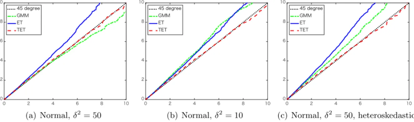
We compare the proposed TET statistic Tn,cet in (11) with the Wald statistic based on the GMM estimator and exponential tilting (ET) statistic Tn,cet in (10). All the statistics converge in distribution to the χ21 distribution under H0. Figure 2 reports the q-q plots of the empirical
quantiles of these test statistics against those of theχ21 distribution for the cases (i)-(iii). Overall, the empirical quantiles of the TET statistic are very close to those of the limiting distribution. These q-q plots of the TET statistics are not sensitive to weaker instruments (as shown in Figure 2(b)) or asymmetric error distributions (as shown in Figure 2(c)). On the other hand, the quantiles of the conventional Wald and ET statistics tend to be larger than the ones of the limiting distribution. In particular, the Wald statistic is worse for all the cases. Such patterns of the q-q plots for the Wald and ET statistics are commonly observed in the literature
(e.g., Imbens, Spady and Johnson, 1998).5 Interestingly, the weaker instruments induce more severe size distortions for the Wald test (see Figure 2(b)).
We also investigate the power properties of the tests for H0 : θ2 = 0 under the alternative
hypotheses H1 :θ2 = 0 + ∆ for different values of ∆. Figures 3 displays the calibrated power
curves of all the tests at5%significance level (i.e., the rejection frequencies of these tests, where the critical values are given by the Monte Carlo 95th percentiles of these test statistics underH0)
for the cases (i)-(iii). The results suggest that the proposed TET tests exhibit good calibrated power. Indeed the calibrated power curves of the TET are very close to those of the ET, and do not show declining power for some negative values of ∆as in the Wald test.
4.2 Specification testing
Second, as an illustration for specification testing in Section 3.2, we consider testing the overi-dentifying restrictionsH0:E[Z(Y−θX)] = 0for someθ againstH1:E[Z(Y −θX)]6= 0 for any θ. We compare the proposed TET statistic Tn,vtet in (13) with the J-statistic based on GMM,6 and ET statistic Tn,vet in (12). All the statistics converge in distribution to the χ21 distribution underH0.
In addition to the cases (i) and (ii) above, we consider the case of heteroskedastic error terms (iv) Yi =θ1+θ2Xi +|Zi|Ui, 1i, 2i ∼ N(0,1), and δ2 = 50. Figure 4 reports the q-q plots of
the empirical quantiles of these test statistics against those of theχ21 distribution for the normal disturbance case.
Although the patterns of the plots are different, we obtain similar conclusions as the simu-lations for composite hypothesis testing. Overall, the empirical quantiles of the TET statistic are very close to those of the limiting distribution compared to the ET and J statistics. The performances of the ET and J statistics are comparable. It is interesting to note that the q-q plots of the TET statistic are not sensitive to heteroskedastic error terms. On the other hand, we can see that heteroskedastic errors deteriorate the size properties of the ET and J statistics. Overall, our simulation results are encouraging: the TET statistic performs excellently com-pared to the existing statistics.
5In the working paper version (available at: http://sticerd.lse.ac.uk/dps/em/em593.pdf), we also report the results for the case of n= 80 and the empirical cumulative distribution functions (ECDFs) of the p-values for all the tests considered in Figures 2 and 4 below. The accuracy of the ET statistic improves as the sample size increases. However, the TET always outperforms the ET and Wald. Furthermore, based on the ECDFs for the p-values, we can see the degrees of size distortions of these statistics. As consistent with the q-q plots, the asymptotic test by the TET shows better size properties (particularly for the region of nominal sizes less than
0.10) than other asymptotic tests. 6Lettingg(W
i, θ) =Zi(Yi−θXi)and¯g(θ) =n−1Pni=1g(Wi, θ), the version of the J-test statistic considered here isJ=nminθ¯g(θ)0[n−1Pni=1g(Wi,θˇ)gWi,θˇ)]−1¯g(θ), whereθˇis the two stage least square estimator.
4.3 Additional results: Weak instruments
Finally, we consider the situation where the instrumental variable Z is very weak (i.e., δ2 = 5
and 1). There is no guarantee that the proposed TET statistic works well under the partial or weak identification; see, Phillips (1989), Staiger and Stock (1997), or Phillips (1980) for an exact analysis with Gaussian errors. In particular, the full rank conditions for the Jacobians of
g (with respect to partially or weakly identified parameters) in Assumptions 1’ and 1” typically fail, and our asymptotic approximations will be invalid. Although its theoretical analysis is left for future research, we here illustrate finite sample performances of the TET statistic under weak instruments.
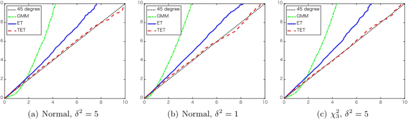
Specifically, we consider three cases: (i’)1i, 2i ∼N(0,1) and δ2 = 5, (ii’)1i, 2i ∼N(0,1)
andδ2 = 1, and (iii’)1i, 2i ∼(χ23−3)/
√
6(standardizedχ23) andδ2 = 5. Figures 5 and 6 report the q-q plots of the empirical quantiles of the test statistics against those of the χ21 distribution for testing H0 : θ2 = 0 and H0 : θ1 = 0, respectively. We note that for testing H0 : θ1 = 0,
the nuisance parameter θ2 is weakly identified and we conjecture that the TET test will be
asymptotically invalid based on the existing literature of weak instruments (e.g., Andrews and Stock, 2007, for a survey).
For testingH0:θ2 = 0, where the nuisance parameterθ1 is strongly identified, the q-q plots
in Figure 5 are similar to the ones in Figure 2, and the TET statistics are not sensitive to very weak instruments. However, for testing H0 :θ1= 0, where the nuisance parameterθ2 is weakly
identified, the q-q plots in Figure 6 suggest that the quantiles of the TET statistics deviate from the ones of the χ2 limiting distribution.7 In particular, the TET is worse than other statistics for the case (ii’). It is an interesting direction of future research to see whether the TET statistic can be modified to be robust to weak instruments or identification.
5
Conclusion
In this paper, we modify the exponential tilting statistic by introducing additional tilting weights to estimate cumulant functions, and propose a novel statistic, called the tilted exponential tilting (TET) statistic. Simulation studies show that the asymptotic p-values of the TET statistic are highly accurate in the tails, and we provide a theoretical explanation for this accuracy by ana-lyzing its relative error properties for the approximation of tail area probabilities. In particular, the proposedp-values accurately approximate those of an infeasible saddlepoint statistic, which
7
In the preliminary simulation study, we considered overidentification testing under the cases (i’)-(iii’). The q-q plots also indicate that the TET statistic for overidentifying restrictions is not robust to very weak instruments.
has relative errors of ordern−1both in normal and large deviation regions. Our TET test allows both just- and over-identified moment condition models, and can be applied for both (possibly composite) parameter hypotheses and overidentifying restriction testing problems.
There are at least two important directions for future research. First, as repeatedly men-tioned, the present analysis lacks theoretical evaluations of closeness of the p-values for the infeasible statistic to the ones for the proposed TET statistic. Although it is a substantial challenge given the existing results of saddlepoint approximations, this theoretical gap should be addressed. Another interesting direction is to investigate theoretical properties of the TET statistic under weak and/or many moment conditions, and to develop a modified statistic that is not only accurate in the tails but also robust to weak and/or many moment conditions.
A
Proofs
A.1 Proof of Theorem 1
Letgi =g(Xi,0). Using Pni=1πˆi = 1 and Pni=1πˆigi = 0, an expansion aroundλˆ = 0implies
nTntet=nˆλ0 " n X i=1 ˆ πie ¯ λ0g ig ig0i # ˆ λ,
where ¯λis a point on the line joining λˆ and 0. LetMˆ =−n1Pn
j=1e ˆ λ0gj. An expansion around ˆ M =−1implies nTntet = −Mˆ−1nˆλ0 " 1 n n X i=1 e(ˆλ+¯λ)0gig ig0i # ˆ λ = nλˆ0 " 1 n n X i=1 e(ˆλ+¯λ)0gig igi0 # ˆ λ+ ¯M−2nˆλ0 " 1 n n X i=1 e(ˆλ+¯λ)0gig ig0i # ˆ λ( ˆM+ 1) = T1+T2,
where M¯ is a point on the line joining Mˆ and −1. By applying the argument in Newey and Smith (2004, pp. 239-240), we can showmax1≤i≤n| −e
ˆ λ0g i+ 1|→p 0andmax 1≤i≤n|e ¯ λ0g i+ 1|→p 0. An expansion of Pn i=1e ˆ λ0gig i= 0 aroundλˆ= 0 implies ˆ λ=− 1 n n X i=1 gig0i !−1 1 n n X i=1 gi ! +op(n−1/2).
Combining these results,
T1= 1 √ n n X i=1 gi !0 1 n n X i=1 gig0i !−1 1 √ n n X i=1 gi ! +op(1)→d χ2p. Finally, by max1≤i≤n| −eλˆ 0g
i + 1|→p 0, it holds Mˆ + 1 →p 0 and then T
2
p
→ 0. Therefore, the conclusion follows.
A.2 Proof of Theorem 2
The basic idea of the proof is similar to that of Robinson, Ronchetti and Young (2003, Theorem 1). Let m(λ) = logE[eλ
0ˇg(X)
is approximated as Pr{nTn≥nt:F}= Pr{2m(ˇλ)≥t:F} = ˆ {y:2m(y)≥t} n 2π p/2 e−nh(y)pdetB(y) det Σ(y)dy(1 +O(n −1)) ≡ A(1 +O(n−1)). (15)
To evaluate the integral A, consider the polar transformation y 7→ (r, s) (with radius r and angle s) and another transformation (r, s) 7→ (u, s) with u= p2m(y). The Jacobians of these transformations are J1(y) = (y0y) p−1 2 and J2(y) = √ y0y√2m(y) m1(y)0y , respectively, where m1(y) =
dm(y)/dy. Define the transformy7→(u, s) asy=ϕ(u, s). By the change of variables, the above integral is written as A= ˆ ∞ √ t cnup−1e−nu 2/2ˆ S δ(u, s)ds du, (16)
wherecn=np/2/(2p/2−1Γ(p/2)),S is the p-dimensional unit sphere, and
δ(u, s) = e nu2/2−nh(ϕ(u,s)) Γ(p/2) 2πp/2up−1 detB(ϕ(u, s)) p det Σ(ϕ(u, s))J1(ϕ(u, s))J2(ϕ(u, s)).
We expand each term inδ(u, s). First, note that
detB(ϕ(u, s)) = detB(0){1 +rξ1(s) +r2R1(r, s)}, 1 p det Σ(ϕ(u, s)) = 1 p det Σ(0){1 +rξ2(s) +r 2R 2(r, s)},
where ξ1 and ξ2 are linear combinations of components of s, and R1 and R2 are uniformly
bounded for r bounded. Due to the normalization E[ˇg(X)ˇg(X)0] = I, we have √detB(0)
det Σ(0) = 1.
Thus, other terms are expanded as
enu2/2−nh(ϕ(u,s)) = 1 +r2R3(r, s),
J1(y) = rp−1,
J2(y) = 1 +rξ4(s) +r2R4(r, s),
u = r{1 +rξ5(s) +r2R5(r, s)},
where ξ4 and ξ5 are linear combinations of terms of the form sisjsk, and R3, R4 and R5 are
uniformly bounded for r bounded. Combining all these expansions,
δ(u, s) = Γ(p/2)
2πp/2 {1 +ub(s) +u 2R
whereR6 is uniformly bounded forr bounded, andb(s)is a linear combination of odd functions
satisfying ´Sb(s)ds= 0. Integrating over the sphere gives
G(u)≡ ˆ
S
δ(u, s)ds= 1 +u2k(u), (17)
for some k(u) bounded overu∈(0, ε). Also we can see thatdG(u)/du=uk1(u) for some k1(u)
bounded over u∈(0, ε). From (15)-(17), Pr{nTn≥nt:F} = ˆ ∞ √ t cnup−1e−nu 2/2 G(u)du(1 +O(n−1)) = ˆ ∞ √ t cnup−1e−n(u−logG(u)/(nu)) 2/2 du(1 +O(n−1)),
where the second equality follows from boundedness of k(u) and k1(u). The conclusion follows
by the change of variables v=u−logG(u)/(nu) and boundedness ofk(u) and k1(u).
A.3 Proof of Theorem 3
Using (15)-(17) in the proof of Theorem 2 and integration by parts, we have
1−Fp(nξ(K(λ))) ={1−Fp(nK(λ))}(1 +O(n−1)) + cn nK(λ) p 2e− nK(λ) 2 " G(pK(λ))−1 K(λ) # . (18)
For the first term on the right hand side of (18), the mean-value theorem yields
1−Fp(nK(λ)) ={1−Fp(nKtet(λ))}(1 +r1n(λ)), where r1n(λ) = e−uλ/¯ 2u¯p/2−1 λ 2p/2Γ(p/2) nKtet(λ)−nK(λ)
1−Fp(nKtet(λ)) for some u¯λ between nK(λ) and nK
tet(λ). For the
second term on the right hand side of (18), let
r2n(λ) = cn nK(λ) p 2e− nK(λ) 2 " G(pK(λ))−1 K(λ) # (1−Fp(nKtet(λ)))−1. Thus, letting rn(λ) =r1n(λ) +r2n(λ), (19) (18) can be written as 1−Fp(nξ(K(λ))) ={1−Fp(nKtet(λ))}(1 +rn(λ))(1 +O(n−1)).
Let R1n(λ), R2n(λ), and Rn(λ) be the sample counterparts of r1n(λ), r2n(λ), and rn(λ),
respectively, obtained by replacingKtet(λ)withKˆtet(λ). It remains to characterize the stochastic order ofRn(λ). Note that the χ2p distribution satisfies
Pr{χ2p ≥u}= 1−Fp(u)≥Ce−u/2up/2−1, (20)
for some constant C >0.
ForR1n(λ), by using (20), we have
|R1n(λ)| ≤Op(1){nKˆtet(λ)−nK(λ)}=Op(n1/2|λ|2),
where Kˆtet(λ) = log Pn i=1πˆieλ 0g(X i,0)
is the sample counterpart of Ktet(λ), and the equality follows from (8) and Pn
i=1πˆig(Xi,0)g(Xi,0)0−E[g(X,0)g(X,0)0] =Op(n1/2).
We now consider R2n(λ). By the definition of G(u) = 1 +u2k(u) for some k(u) bounded
over u ∈ (0, ε), G( √ K(λ))−1 K(λ)
is also bounded. Thus, by using (20) and the definition of cn =
np/2/(2p/2−1Γ(p/2)), we have
|R2n(λ)| ≤Op(1) ˆKtet(λ) =Op(|λ|2).
Combining these results, we obtain the conclusionRn(λ) =Op(n1/2|λ|2).
A.4 Proof of Theorem 4
Proof of Part (i)
LetΩ =E[g(X, θ0)g(X, θ0)0]andM = Ω−1/2E[∂g(X, θ0)/∂θ10]. By the spectral decomposition of
the idempotent matrix (Czellar and Ronchetti, 2010), there exists a matrix C = [C1 :C2]such
that M(M0M)−1M0=C Ip1 0 0 0p2×p2 C 0,
and C0C =CC0 =Ip withp=p1+p2. Based on Newey and Smith (2004, p. 240), we can see
that √nλ˜ is asymptotically equivalent to√nΩ−1/2C2˜γ, whereγ˜ solves
n X i=1 e˜γ0˜g(Xi,θ0)˜g(X i, θ0) = 0, where ˜ g(X, θ0) =C20Ω−1/2g(X, θ0). (21)
The saddlepoint density of ˜γ is given by (6) with replacement of g(Xi, θ0) with ˜g(Xi, θ0). Let ˜
K(γ) =K(Ω−1/2C2γ,θ˜1(Ω−1/2C2γ)). We can also see that
Pr{nTn,c≥ntn,c:F}= Pr{2nK˜(˜γ)≥nK˜(˜γo) :F}(1 +O(e−n)),
for any >0small enough. Then the conclusion follows as in the proof of Theorem 2 by replacing
hλ(y) = logE[ey
0g(X,0)
]withlogE[ey
0˜g(X,θ
0)].
Proof of Part (ii)
Using the spectral decomposition of idempotent matrix adopted in the proof of (i), we can show that nKtet(λ,θ˜tet1 (λ))−nK(λ,θ˜1(λ)) = O(n1/2|λ|2). Therefore, (ii) follows by using the same
arguments adopted for the proof of Theorem 3.
A.5 Proof of Theorem 5
B
Figures for Section 4
(a) Normal,δ2= 50 (b) Normal,δ2= 10 (c)χ23,δ2= 50
Figure 2: q-q plots for H0 :θ2 = 0withn= 40: (a) Normal,δ2 = 50, (b) Normal,δ2 = 10, and
(c) χ23,δ2= 50.
(a) Normal,δ2= 50 (b) Normal,δ2= 10 (c)χ23,δ2= 50
Figure 3: Calibrated powers for H0 : θ2 = 0 with n = 40: (a) Normal, δ2 = 50, (b) Normal,
δ2 = 10, and (c) χ23,δ2= 50.
(a) Normal,δ2= 50 (b) Normal,δ2= 10 (c) Normal,δ2= 50, heteroskedastic
Figure 4: q-q plots for overidentification withn= 40: (a) Normal, δ2= 50, (b) Normal,δ2= 10, and (c) Normal, δ2 = 50, heteroskedastic.
(a) Normal,δ2= 5 (b) Normal,δ2= 1 (c)χ2 3,δ2= 5
Figure 5: q-q plots forH0 :θ2 = 0 withn= 40: (a) Normal,δ2 = 5, (b) Normal,δ2= 1, and (c)
χ23,δ2 = 5.
(a) Normal,δ2= 5
(b) Normal,δ2= 1
(c)χ2 3,δ2= 5
Figure 6: q-q plots forH0 :θ1 = 0 withn= 40: (a) Normal,δ2 = 5, (b) Normal,δ2= 1, and (c)
References
[1] Almudevar, A., Field, C. and J. Robinson (2000) The density of multivariate M-estimates, Annals of Statistics, 28, 275-297.
[2] Andrews, D. W. K. and J. H. Stock (2007) Inference with weak instruments, in Advances in Economics and Econometrics, Theory and Applications, Ninth World Congress, vol. 3, Blundell, R., Newey, W. and T. Persson (eds.), Cambridge University Press, pp. 122-173. [3] Baggerly, K. A. (1998) Empirical likelihood as a goodness-of-fit measure, Biometrika, 85,
535-547.
[4] Brown, B. W. and W. K. Newey (1998) Efficient semiparametric estimation of expectations, Econometrica, 66, 453-464.
[5] Czellar, V. and E. Ronchetti (2010) Accurate and robust tests for indirect inference, Biometrika, 97, 621-630.
[6] Daniels, H. E. and G. A. Young (1991) Saddlepoint approximation for the studentized mean, with an application to the bootstrap,Biometrika, 78, 169-179.
[7] Efron, B. (1981) Nonparametric standard errors and confidence intervals, Canadian Journal of Statistics, 9, 139-172.
[8] Efron, B. (1982) Transformation theory: How normal is a family of distributions?, Annals of Statistics, 10, 323-339.
[9] DiCiccio, T. J., Hall, P. and J. Romano (1991) Empirical likelihood is Bartlett-correctable, Annals of Statistics, 19, 1053-1061.
[10] Field, C. A. (1982) Small sample asymptotic expansions for multivariate M-estimates, An-nals of Statistics, 10, 672-689.
[11] Huber, P. J. and E. M. Ronchetti (2009) Robust Statistics, 2nd edition, Wiley.
[12] Imbens, G. W., Spady, R. H. and P. Johnson (1998) Information theoretic approaches to inference in moment condition models, Econometrica, 66, 333-357.
[13] Jensen, J. L. (1995) Saddlepoint Approximations, Oxford University Press.
[14] Jensen, J. L. and A. T. A. Wood (1998) Large deviation and other results for minimum contrast estimators,Annals of the Institute of Mathematical Statistics, 50, 673-695.
[15] Jing, B. Y. and J. Robinson (1994) Saddlepoint approximations for marginal and conditional probabilities of transformed variables,Annals of Statistics, 22, 1115-1132.
[16] Jing, B. Y., Shao, Q. M. and W. Zhou (2004) Saddlepoint approximation for student’s t-statistic with no moment conditions,Annals of Statistics, 32, 2697-2711.
[17] Jing, B. Y. and A. T. A. Wood (1996) Exponential empirical likelihood is not Bartlett correctable,Annals of Statistics, 24, 365-369.
[18] Kitamura, Y. (2007) Empirical likelihood methods in econometrics: theory and practice, in Blundell, R., Newey, W. K. and T. Persson (eds.),Advances in Economics and Econometrics, vol. III, 174-237.
[19] Kitamura, Y. and M. Stutzer (1997) An information-theoretic alternative to generalized method of moments estimation,Econometrica, 65, 861-874.
[20] Kolassa, J. and J. Robinson (2011) Saddlepoint approximations for likelihood ratio like statistics with applications to permutation tests,Annals of Statistics, 39, 3357-3368. [21] Ma, Y. and E. Ronchetti (2011) Saddlepoint test in measurement error models, Journal of
the American Statistical Association, 106, 147-156.
[22] Newey, W. K. and R. J. Smith (2004) Higher order properties of GMM and generalized empirical likelihood estimators,Econometrica, 72, 219-255.
[23] Owen, A. B. (1988) Empirical likelihood ratio confidence intervals for a single functional, Biometrika, 75, 237-249.
[24] Owen, A. B. (2001) Empirical Likelihood, New York, Chapman and Hall.
[25] Phillips, P. C. B. (1980) The exact distribution of instrumental variable estimators in an equation containingn+ 1endogenous variables, Econometrica, 48, 861-878.
[26] Phillips, P. C. B. (1989) Partially identified econometric models, Econometric Theory, 5, 181-240.
[27] Robinson, J., Ronchetti, E. and G. A. Young (2003) Saddlepoint approximations and tests based on multivariate M-estimates,Annals of Statistics, 31, 1154-1169.
[28] Skovgaard, I. M. (1990) On the density of minimum contrast estimators,Annals of Statistics, 18, 779-789.
[29] Staiger, D. and J. H. Stock (1997) Instrumental variables regression with weak instruments, Econometrica, 65, 557-586.
[30] Tingley, M. A. and C. A. Field (1990) Small-sample confidence intervals, Journal of the American Statistical Association, 85, 427-434.