Contents lists available atScienceDirect
Journal of Multivariate Analysis
journal homepage:www.elsevier.com/locate/jmva
√
n
-Consistent robust integration-based estimation
Sung Jae Jun
∗, Joris Pinkse, Yuanyuan Wan
Center for the Study of Auctions, Procurements and Competition Policy, Department of Economics, The Pennsylvania State University, United States
a r t i c l e i n f o Article history:
Received 14 June 2010 Available online 8 January 2011 AMS subject classifications: 62F10 62F35 62J05 Keywords: Robust regression Linear model Integration-based estimator High breakdown point estimator
a b s t r a c t
We propose a new robust estimator of the regression coefficients in a linear regression model. The proposed estimator is the only robust estimator based on integration rather than optimization. It allows for dependence between errors and regressors, is √n -consistent, and asymptotically normal. Moreover, it has the best achievablebreakdown point of regression invariant estimators, has bounded gross error sensitivity, is both affine invariant andregression invariant, and the number of operations required for its computation is linear inn. An extension would result in boundedlocal shift sensitivity,also.
©2011 Elsevier Inc. All rights reserved.
1. Introduction
We propose a new estimator for the regression coefficients in a linear regression model, which is robust to ‘contamination’. Our estimator is inspired by theleast median of squares(LMS) estimator of Rousseeuw [27] and theLaplace estimator of Chernozhukov and Hong [3]; see also Jun et al. [18]. Like Laplace estimators, our estimator is defined as the ratio of two integrals involving an exponential transform of (in our case) the LMS objective function, but this is where the similarity ends.
Suppose that the parameter vector of interest
θ
0is the unique minimizer of a population objective functionΩ over a compact parameter spaceΘ. Laplace estimators then employ the fact thatθ
0satisfiesθ
0=
lim n→∞
θϖ (θ)
exp{−
α
nΩ(θ)
}
dθ
ϖ (θ)
exp{−
α
nΩ(θ)
}
dθ
,
(1.1)where
ϖ
is a pseudo-prior defined onΘand{
α
n}
is a scalar-valued deterministic sequence diverging to infinity with the sample sizen. Note here that the densityϖ (θ)
exp{−
α
nΩ(θ)
}
/
ϖ (θ)
exp{−
α
nΩ(θ)
}
dθ
becomes more concentrated aroundθ
0 asα
n increases. ReplacingΩ in(1.1)with its sample analogΩˆ
1 results in a Laplace estimator. If a quadratic expansion ofΩˆ
is available then the Laplace estimator is generally√
n-consistent [3] and the divergence rate ofα
nis of lesser importance. In the absence of such a quadratic expansion, as in the case of the LMS estimator, the resulting estimator is not√
n-consistent, and the divergence rate ofα
npartly determines the convergence rate of the Laplace estimator [18].We, instead, use the fact that in our caseΩis symmetric around
θ
0, which implies thatθ
0=
θ
exp{−
Ω(θ)
}
dθ
exp
{−
Ω(θ)
}
dθ
,
(1.2)∗Corresponding address: 303 Kern Graduate Building, University Park, PA 16802, United States.
E-mail addresses:[email protected],[email protected](S.J. Jun),[email protected](J. Pinkse),[email protected](Y. Wan). 1 We use bold face for random variables.
0047-259X/$ – see front matter©2011 Elsevier Inc. All rights reserved.
Table 1
Comparison of robust estimators of the coefficients in a linear regression model.
Estimation method Acronym BDP=0.5 GES finite LSS finite √n
rate
Normal Comp. #
oper.
Equivariance
Scale Affine Regr.
Huber [17] HUB ✓ ✓ ? ✓ ✓
Koenker and Bassett [21] LAD ✓ ✓ n a ✓ ✓ ✓
Krasker [22] HK ✓ ✓ ✓ ? ✓ ✓ Siegel [32]b RM ✓ ✓ ✓ ✓ nd c ✓ ✓ Mallows [23] MAL ✓ ✓ ✓ ✓ ? ✓ ✓ Rousseeuw [27] LMS ✓ ✓d nd e ✓ ✓ ✓ Rousseeuw [27] LTS ✓ ✓ ✓ ✓ nlogn ✓ ✓ ✓ Rousseeuw and Yohai [29] SEST ✓ ✓ ✓ n2logn ✓ ✓ ✓ Yohai [33] MM ✓ ✓ ✓ ? ✓ ✓
Yohai and Zamar [34] TAU ✓ ✓ ✓ ? ✓ ✓
Croux et al. [5] GS ✓ ✓ ✓ n2logn f
✓ ✓
Hossjer [16] LTA ✓ ✓ ✓ ✓ nlogn ✓ ✓ ✓
Chang et al. [2] HBRR ✓ ✓g ? ✓ ✓ ? ✓ ✓ ✓
Zinde-Walsh [35] SLMS ✓ ✓ ? ✓ ✓
Čížek [4] GTE ✓ ✓ ✓ ✓ ? ✓ ✓ ✓
New ✓ ✓ h ✓ ✓ n ✓ ✓
aWith preprocessing; see Portnoy and Koenker [24]. b Asymptotics are due to Hossjer [16].
c dis the number of regressors.
d If the constant is not varied, infinite if varied; see Davies [7]. eSee Croux et al. [5].
f See Croux et al. [5];dis the number of regressors. gIf the constant is not varied.
h Can be modified to have a finite LSS.
where the integrals are taken over the entire Euclidean space. There are four fundamental differences between(1.1)and (1.2): in(1.2)there is no limit, there is no
α
n, there is no compact parameter space requirement, and there is noϖ
. As there is no limit in(1.2),α
nis not needed anymore. Since the symmetry ofΩaroundθ
0is used, the parameter space should not be artificially restricted and no prior can be used. Our estimatorθ
ˆ
is obtained by replacingΩin(1.2)withΩˆ
.In this paper we focus our attention on the case in whichΩ
ˆ
is the LMS objective function, or a close relative thereof.We show that, subject to assumptions outlined in subsequent sections,
θ
ˆ
is√
n-consistent and asymptotically normal with many robustness properties, which will be further explained below. Please note that although our estimator resembles a Bayes estimator, it is quite different in that withΩˆ
being the LMS objective function, exp(
− ˆ
Ω)
is not a likelihood.Instead of basing an estimator on(1.2), as we do in this paper, one could alternatively consider
θ
ˆ
L, the Laplace estimator usingΩˆ
. However, as the LMS objective function does not allow for a quadratic expansion [19],θ
ˆ
Lwill not be√
n-consistent. Indeed, this scenario is similar to the one studied in [18] for the objective functions of other
√
3n-consistent estimators. The pioneering work of Huber [17] has spawned an abundance of papers proposing estimators with ever more desirable robustness properties. The main differences between the estimators are their robustness properties, their asymptotic behavior absent contamination, their equivariance properties, and their degree of computational complexity. These properties are summarized inTable 1. Our estimator is attractive in all four respects, as the exposition below will make apparent.
One notion of robustness is the finite samplebreakdown point[8],2which is the fraction of the sample that must be changed to push the value of an estimator arbitrarily far. The breakdown point of the least squares estimator equals 1
/
nand the breakdown point of the least absolute deviations estimator [21] depends on the regressor distribution and can be arbitrarily close to zero in large samples [15, p. 328]. Most estimators, however, have a finite sample breakdown point close to 0.5 if the regressors are ingeneral position[27]. Notable exceptions are Huber [17], Krasker [22], Mallows [23]. Our estimator has the best achievable breakdown point of regression invariant estimators, determined in [27].
Since the requirement that regressors are in general position is strong, we provide results that are more general than that. Specifically, it can be preferable (from a breakdown point perspective) to use a quantileqother than the median. Details can be found in Section3.
Other commonly used notions of robustness are thegross error sensitivity(GES) and thelocal shift sensitivity(LSS), both due to Hampel [12,14]. The GES of an estimator is finite if itsinfluence function[12,14] is bounded. Many, but not all, robust estimators have a bounded influence function, including ours.
The LSS is finite if the partial derivative of the influence function with respect to regressor and regressand values is bounded.3We know of only one estimator, namely Mallows [23], which is known to have a finite LSS. The proposed estimator
2 An asymptotic version can be found in [13] and a different breakdown point concept in [30,31]. 3 The definition of the LSS is more general in that it allows for left and right derivatives to be different.
does not have a finite LSS if the tails of the error distribution are thin. We do, however, describe a modification of our estimator which can achieve a finite LSS.
Virtually all existing robust estimators, and ours, are
√
n-consistent and asymptotically normal. The two exceptions are the other two LMS-based estimators, Rousseeuw [27], Zinde-Walsh [35]. The original LMS estimator has been shown to be 3√
n-consistent and has a complicated limit distribution [19, see]. Zinde-Walsh [35] smoothes out the LMS objective function to obtain a better convergence rate and a limiting normal distribution, but her estimator does not achieve the desired
√
n -rate and its GES is infinite.Like Zinde-Walsh [35], but unlike most of the other estimators mentioned here, we do allow for dependence between errors and regressors. There are many examples in economics in which e.g. heteroskedasticity is important. Unlike Zinde-Walsh [35], however, we do not allow for time series dependence, but follow the rest of the literature and assume independent and identically distributed (i.i.d.) data.
Almost all existing estimators, and ours, are bothaffine invariantandregression invariant.About half of them are also
scale invariant,meaning that if the regressand is scaled, the vector of regression coefficient estimates is scaled by the same amount. Our estimator is not scale invariant, and scaling does have a material impact on its performance. Issues pertaining to scaling are discussed in detail in Section6.
Finally, there is great variation in the computational complexity of estimators, both in terms of computation time and the difficulty of writing a program. Ours is the only high breakdown point estimator for which the number of operations required for its computation is linear inn, albeit that the constant multiplyingncan be large and increases with the number of regressorsd. Since our estimator is the ratio of two integrals, it can be computed using any of a number of numerical integration techniques. For low-dimensional (smalld) problems Gaussian quadrature works well. For many regressors, (quasi) Monte Carlo techniques can be used. For the numbers produced in this paper, we use Gibbs sampling [10]. A simple Gibbs sampling procedure is described inAppendix F; a C program using a faster algorithm is available from the authors upon request.
There are at least two interesting extensions which are not explored in this paper and are left for future work. First, under additional conditions the methodology could potentially be applied to nonlinear regression models, including generalized linear models with a known link function. It is difficult at this point to oversee how restrictive such additional conditions would be or indeed what class of nonlinear regression functions this would work for. Second, our estimator is defined as a
quasi-posteriormean, but one could alternatively look at quantiles of the quasi-posterior distribution; this possibility has already been explored for Laplace estimators by Chernozhukov and Hong [3].
The remainder of our paper is organized as follows. In Section2we define our estimator. Its breakdown point properties are established in Section3. Section4contains the asymptotic results absent contamination and Section5a discussion of its asymptotic robustness properties (GES and LSS). Finally, Section6addresses the effects of scaling of observables and Section7the computation of the proposed estimator.
2. Estimator
For some 0
<
q<
1 to be chosen, letN= ⌊
qn⌋ +
1, where⌊·⌋
denotes the largest integer no greater than its argument. Let furtherQ∗(ξ
;
q∗)
denote theq∗-quantile of the distribution ofξ
,Q(ξ)
=
Q∗(ξ
;
q)
, and letQˆ
(ξ
i
)
be theNth order statistic ofξ
1, . . .
ξ
nfor arbitraryξ
’s; soQ,
Qˆ
are population and sample quantiles, respectively. In case a quantile is not unique, inthe sense that there are multiple valuesmthat satisfyP
(ξ
<
m)
≤
q≤
1−
P(ξ
>
m),
Qis taken to be any such value.4 Let{
(
xi,
yi)
}
be an i.i.d. sample of sizenwherexi∈
Rd. The object of interest is the vector of regression coefficients inthe linear regression model
yi
=
x|iθ
0+
ui,
i=
1, . . . ,
n.
Under conditions to be developed in Section4,
θ
0is unique and given byθ
0=
argmin θ∈Rd Q(
|
yi−
x|iθ
|
2).
(2.1) Our estimator ofθ
0isˆ
θ
=
θ
exp{− ˆ
Q(
|
yi−
x|iθ
|
2)
}
dθ
exp{− ˆ
Q(
|
yi−
x|iθ
|
2)
}
dθ
.
(2.2)The estimator
θ
ˆ
resembles a Laplace estimator [3,18], albeit that (mentioned in the Introduction) there is no sample-size-dependent input parameter scaling the objective function and no pseudo-prior. Indeed, in [3,18] the objective function must be multiplied by a parameter which tends to infinity with the sample size to ensure consistency; in [3] the parameter is set ton, in [18] it is chosen by the practitioner. This is not needed here becausem(
t)
=
Q{|
yi−
x|i(θ
0+
t)
|}
happens to be symmetric int.By substitution oft
=
θ
−
θ
0in(2.2)it follows that formˆ
n(
t)
= ˆ
Q{|
yi−
x|i(θ
0+
t)
|}
,ˆ
θ
−
θ
0=
texp{− ˆ
m2n(
t)
}
dt
exp{− ˆ
m2 n(
t)
}
dt.
(2.3)The representation(2.3)will be frequently used in the remainder of this paper, especially in the proofs. 3. Breakdown point
We now establish a general result concerning the breakdown properties of our estimator, which implies that the breakdown properties of our estimator are no worse than those of Rousseeuw [27].
LetY
ˆ
n=
sup‖t‖=1n−1∑
ni=1I
(
|
x |it
| =
0),
γ
ˆ
=
nYˆ
nandY=
sup‖t‖=1P(
|
x|it| =
0)
. The numbersYˆ
n,
γ
ˆ
represent the degree of noncollinearity in the sample andY that in the population. The best breakdown point obtains when observations are ingeneral position[27], in which caseγ
ˆ
=
d−
1. However, becauseY>
0 if one (or more) of the regressors other than the constant is discrete, the general position property then occurs with probability approaching zero asn→ ∞
. Our breakdown point result is hence for genericγ
ˆ
.Theorem 1.If
γ
ˆ
+
1<
N<
n then the breakdown pointbˆ
ofθ
ˆ
satisfiesbˆ
≥ {
min(
n−
N,
N− ˆ
γ
−
1)
+
1}
/
n.Theorem 1only provides a lower bound to the breakdown point. It is straightforward to construct examples in which
ˆ
b
= {
min(
n−
N,
N− ˆ
γ
−
1)
+
1}
/
n.Theorem 1has several implications. First, forq
=
0.
5, the breakdown point when the observations are in general position is(
⌊
n/
2⌋ −
d+
2)/
nifd>
1,5which is exactly the same as in [27, theorem 1]. The best breakdown point is achieved whenqis chosen to makeN
= ⌊
(
n+ ˆ
γ
+
1)/
2⌋
, which results in a breakdown point of⌊
(
n− ˆ
γ
+
1)/
2⌋
/
n. If the observations are in general position then the breakdown point equals⌊
(
n−
d)/
2⌋ +
1, which is the same as that in the remark following Theorem 1 of Rousseeuw [27] and hence also as that of Siegel [32].Asymptotically, the optimal choice ofqin terms of breakdown properties is
q
=
1+
Y2
,
(3.1)resulting in a breakdown point converging to
(
1−
Y)/
2 asn→ ∞
, which is the best achievable for any regression equivariant estimator [27]. The rationale for the choice ofqin(3.1)is thatYˆ
n→
p Y and hence thatγ
ˆ
≈
nY, resulting in an optimalNof≈
n(
1+
Y)/
2.4. Asymptotics
We now turn to a discussion of the properties of
θ
ˆ
absent contamination. Throughout we assume that{
(
xi,
yi)
}
is an i.i.d. sequence of random variables and that 0<
q<
1.We start by establishing identification. Letm0
=
Q(
|
yi−
x|iθ
0|
)
=
Q(
|
ui|
)
.Assumption A. The conditional densityf
(
·|·
)
ofuigivenxi=
xis for anyxeven, continuous, positive on the entire real line, weakly decreasing at allu>
0, and strictly decreasing atm0.Assumption Ais strong, but forq
=
0.
5 weaker than [19, Example 6.3] because we allowuiandxito be dependent and do not assume the existence of derivatives for consistency. It is used here to establish identification.Recall from Section3thatY
=
sup‖t‖=1P(
|
x|it| =
0)
.Assumption B. Y
<
1.Assumption Brequires that the regressors are perfectly collinear with probability less than one. It is implied by the requirement that 0
<
E(
xixi|) <
∞
[19, Example 6.3], but does not assume the existence of moments forxi. Given that forY
>
0 regressors are in general position with probability approaching zero (see Section3),Assumption Bis weak. Theorem 2.UnderAssumptionsAandB,θ
0defined in(2.1)is unique.We need one additional condition for consistency. Assumption C. Y
<
q.Assumption Cis the population equivalent (forq
=
0.
5) of the requirement in [27] that novertical hyperplane(passing through the origin) contains more than⌊
n/
2⌋
observations.Assumption Ccan be restrictive. Indeed, with both a constant and a binary regressor it is violated whenq
≤
0.
5. But ifY>
qthen with probability approaching oneYˆ
n>
q, also, and the condition imposed onNinTheorem 1is violated.Consequently, none of the LMS-type estimators, Rousseeuw [27], Zinde-Walsh [35] and ours, will then have a breakdown point any better than the OLS estimator. So ifAssumption Cis violated, it just means thatqis chosen too small. In particular, ifqis chosen according to(3.1)thenAssumption Cis equivalent toAssumption B.
Theorem 3. UnderAssumptionsA–C,
θ
ˆ
→
pθ
0.We now proceed with a discussion of the asymptotic distribution of
θ
ˆ
. Letm
(
t)
=
Q(
|
ui−
x|it|
),
m∞(
t)
=
Q(
|
x|it|
).
(4.1)The notationm∞is inspired by the fact that for anyt
̸=
0,
limλ→∞{
m(λ
t)/λ
} =
m∞(
t)
provided thatm∞(
t)
is unique.Let f
(
·
)
and F(
·
)
be the unconditional counterparts off(
·|·
)
and F(
·|·
)
, and letX=
x: ∃‖
t‖ =
1, ϵ >
0:
|
x|t| −
m∞(
t)
< ϵ
. Assumption D. (i) lim η↓0 inf ‖t‖=1P{|
x|it| ≤
m∞(
t)
+
η
} −
qη
>
0,
limη↓0 inf ‖t‖=1P{|
x|it| ≥
m∞(
t)
−
η
} −
1+
qη
>
0,
where each inequality is taken to hold if the limit is infinite. Moreover, (ii) for some
ϵ >
0,
0<
infxf(ϵ
|
x)
≤
supxf(
0|
x) <
∞
and for some 2<
r<
∞
, (iii) lims→∞{
infx∈Xf(
s|
x)/
fr(
s)
} ≥
1, and(iv) lims→∞
[
f{
s+
F(
−
s)/
f(
s)
}
/
fr(
s)
]
>
0.Conditions (ii) and (iii) inAssumption Dare automatically satisfied ifui andxi are independent and can be seen as mild conditions restricting their dependence. We have verified condition (iv) for a number of distributions satisfying Assumption A, including (symmetrized versions of) the Normal, Gumbel, Laplace, and Cauchy distributions.
Finally, condition (i) is satisfied when all regressors other than the constant are continuous. For discrete distributions, (i) is satisfied for most, but not all, choices ofq. Condition (i) assumes away the possibility that theq-quantile of
|
x|it|
is ambiguous for any vectortof length one. Condition (i) is unique to our paper.Asqcan be chosen to satisfy (i), condition (i) is more a nuisance than a serious obstacle for our estimator. Nevertheless, we highlight two alternatives that can be used to replaceAssumption D. The first solution is to assume that the tails of the conditional error density are sufficiently thick, i.e. declining more slowly than those of the density of an exponential distribution, which is not desirable. The second solution is to replace
|
yi−
x|iθ
|
2in(2.2)withδ(
|
yi−
x|iθ
|
)
withδ
a function increasing much faster than quadratically. We do not provide a formal justification for either solution.6Finally, we need a condition on the derivative off. Assumption E. supu,xf′
(
u|
x) <
∞
.Assumption Eis strong, but the assumption of the existence of the first derivative is also used in [19,16,35], among others. Please note thatAssumption Eis only used to establish asymptotic normality.
LetA
(
t,
m)
=
P(
|
ui−
x|it| ≤
m),
D(
t)
=
∂
mA{
t,
m(
t)
}
,7 H(
t,
s)
=
Cov[
I{|
ui−
x|it| ≤
m(
t)
}
,
I{|
ui−
xi|s| ≤
m(
s)
}]
,
(4.2) and V=
4
ts|m(t)m(s) D(t)D(s)H(
t,
s)
exp[−{
m 2(
t)
+
m2(
s)
}]
dtds
exp{−
m2(
t)
}
dt
2.
(4.3)Theorem 4. LetAssumptionsA–Ehold. Then
√
n(
θ
ˆ
−
θ
0)
→
d N(
0,
V)
.So even though the original LMS estimator is
√
3n-consistent like other estimators studied by Kim and Pollard [19], the convergence rate in the LMS case can be improved to
√
nwhereas Jun et al. [18] have shown that the convergence rate of Laplace versions of other such estimators crucially depends on the smoothness of the population objective function and is necessarily worse than√
n. The reason is that the functionm, defined in Section2, is even, and that our estimator is asmoothfunctional of the LMS objective function. Indeed,(2.3)shows that the mapping fromm
ˆ
ntoθ
ˆ
−
θ
0is smooth, even though6 Both alternatives ensure thattexp{−m2(t)}/D(t)(or its equivalent ifδis used) in(4.3)is integrable, which is needed. 7 ∂
ˆ
mnitself is not smooth. Consequently, expanding exp
− ˆ
m2n
(
t)
in(2.3)aroundm
(
t)
for eachtsuggests that (the proof of Theorem 4is precise)ˆ
θ
−
θ
0≃
texp{−
m2(
t)
}
dt
exp{−
m2(
t)
}
dt−
2
tm(
t)
{ ˆ
mn(
t)
−
m(
t)
}
exp{−
m2(
t)
}
dt
exp{−
m2(
t)
}
dt,
(4.4) where≃
means that the remainder terms are asymptotically negligible. Here, the second right-hand side term in(4.4)is√
n-normal by a central limit theorem. The ‘bias’ term in(4.4), i.e. the first right-hand side term,equalszero due to the symmetry ofm, whereas the corresponding term in [18] is nonzero and can only be made to converge to zero by expanding the population objective function around zero, introducing the divergent sequence
{
α
n}
mentioned in the Introduction, and (choosing a particular bias-reducing) prior. In other words, in [18] a bit of ‘bias’ is introduced to obtain a more significant reduction in ‘variance’ whereas in the present case the ‘variance reduction’ obtains without generating ‘bias’.8We have shown that our estimator has good breakdown properties and is both
√
n-consistent and asymptotically normal. For the sake of completeness, we now provide a consistent estimatorVˆ
ofV. Letˆ
H∗(θ,
θ)
˜
=
n−1 n−
i=1 I{|
yi−
x|iθ
| ≤ ˆ
Q(
|
yi−
x|iθ
|
)
}
I{|
yi−
x|iθ
˜
| ≤ ˆ
Q(
|
yi−
x|iθ)
˜
}
−
n−1 n−
i=1 I{|
yi−
x|iθ
| ≤ ˆ
Q(
|
yi−
x|iθ
|
)
}
n−1 n−
i=1 I{|
yi−
x|iθ
| ≤ ˆ
Q(
|
yi−
x|iθ
˜
|
)
}
,
(4.5)and for some scalarh∗
(θ)
,ˆ
D∗(θ)
=
1 2nh∗(θ)
n−
i=1 I
|
yi−
x|iθ
| − ˆ
Q(
|
yi−
x|iθ
|
)
≤
h∗(θ)
.
(4.6)Then our estimator of the asymptotic variance is
ˆ
V=
4
(θ
− ˆ
θ)(
θ
˜
− ˆ
θ)
|Qˆ(|yi−xi|θ|)Qˆ(|yi−x|iθ˜|) ˆ D∗(θ)Dˆ∗(θ)˜ Hˆ
∗(θ,
θ)
˜
e−{ ˆQ(|yi−x|iθ|2)+ ˆQ(|yi−x|iθ˜|2)}dθ
dθ
˜
exp{− ˆ
Q(
|
yi−
x|iθ
|
2)
}
dθ
2.
(4.7)The use of a uniformkernelin(4.6)is not essential but simplifies the proofs.
We need a single additional assumption, relating to the choice ofbandwidth h∗. Let
≺
indicate that the left-hand side is of smaller order than the right-hand side and let≼
,
≻
,
≽
be likewise defined.Assumption F. The bandwidth functionh∗satisfiesh∗
(θ)
=
(
1+‖
θ
‖
p∗)
h0for some 2<
p∗<
∞
andh0≺
1≺
n(1−1/p∗)/σ
h0 for some
σ >
4.Becauseh0andp∗are chosen by the practitioner,Assumption Fis not restrictive.Assumption Fpermits the bandwidth to converge at the ‘optimal’n−1/5rate ifp∗
>
5. We are now in a position to state the final theorem of this section. Theorem 5.LetAssumptionsA–Fhold. ThenVˆ
→
p V.5. Influence function
From the proof ofTheorem 49it is apparent that the dominant asymptotic term is 2
√
n n−
i=1
tDm((tt))
I{|
ui−
x|it| ≤
m(
t)
} −
q
exp{−
m2(
t)
}
dt
exp{−
m2(
t)
}
dt,
resulting in the influence function [14]10I
(
y,
x)
=
2
tDm((tt))
I{|
y−
x|(θ
0+
t)
| ≤
m(
t)
} −
q
exp{−
m2(
t)
}
dt
exp{−
m2(
t)
}
dt.
(5.1)Sincey
,
xenter(5.1)only through an indicator function,I is uniformly bounded and the GES11of our estimator is hence finite.8 The terms ‘bias’ and ‘variance’ are used loosely here to refer to whether or not the distribution is approximately correctly centered and variability of the distribution around the center, not in terms of the first two moments of the (dominant asymptotic expansion term of the) estimator.
9 See(E.6).
10 In [14] the influence function is defined as a functional derivative, which generally equals an element in the sum in the first order asymptotic term [25,1,9]. We do not establish such equivalence here.
The LSS is more complicated to determine. We now show that even in the constant-only case, our estimator does not have a finite LSS when the tails of the error distribution are thin.
Theorem 6. Suppose thatxiconsists of only a constant and that F is the distribution function of a mean zero normal random
variable with variance
ς
2. Then if q=
0.
5, ς
2>
2⇐⇒
supy|
∂
yI(
y)
|
<
∞
.As the proof ofTheorem 6illustrates, the LSS is infinite for thin-tailed error distributions, because exp
(
−
m2)
does then not decrease fast enough asmincreases. This problem can be remedied by replacing exp in(2.2)by another smooth function which equals zero whenever its argument is sufficiently large negative. We do not investigate such a modification in this paper.6. Scaling
Like Laplace estimators [3], the proposed estimator is not invariant to scaling, or indeed monotonic transformations, of the objective function. In our case scaling the objective function is equivalent to scaling the data, so consider the estimator
ˆ
θ
αbelow in which the scaling is made explicit by means of a scalar 0< α <
∞
.ˆ
θ
α=
θ
exp{−
α
Qˆ
(
|
yi−
x|iθ
|
2)
}
dθ
exp{−
α
Qˆ
(
|
yi−
x|iθ
|
2)
}
dθ
.
Having
α
be finite and nonzero is important for our results. It is apparent that limα→∞θ
ˆ
α(forq=
0.
5) yields Rousseeuw’sLMS estimator, which is not
√
n-consistent and lacks a bounded influence function unless the supremum is only taken over the slope regressors [7].To obtain the limit of
θ
ˆ
αasα
→
0 is somewhat more complicated. We limit ourselves to the case with oddn, scalar-valued nonnegativexiandq=
0.
5, which is nonetheless instructive.12Letµ
=
(
n+
1)/
2 and let the data be arranged such thatxi<
xj⇒
i<
jandxi≤
xj,
yi<
yj⇒
i<
j.13Theorem 7. Suppose that n is odd, d
=
1,
q=
0.
5, and that there are no ties in theyi-values. If allxi’s are nonnegative and xµ>
0, thenlimα→0θ
ˆ
α=
yµ/
xµ.
Theorem 7has two interesting implications. First, ifxiis a constant thenyµ
/
xµequals the sample median, which has excellent properties. In most other cases, however,yµ/
xµis an inconsistent estimator ofθ
0. Indeed, ifxiis continuously distributed thenyµ/
xµis the ratio of theyandxvalues of the observation corresponding to the sample median of thexi’s.So the value of
α
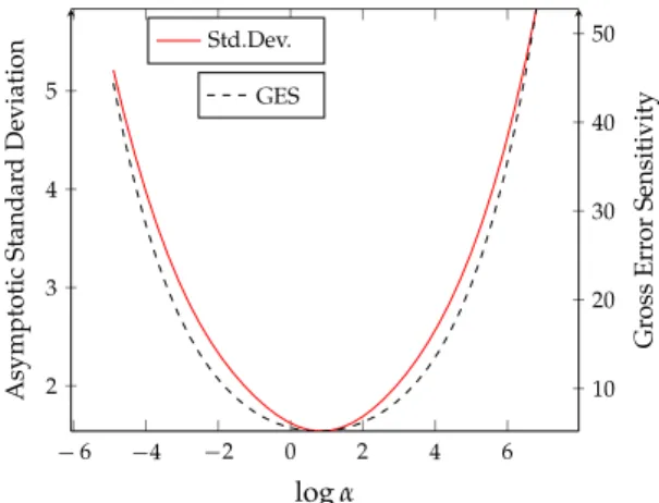
that minimizes the asymptotic variance is generally different from zero and infinity and the same is true for the value that minimizes the gross error sensitivity. Other estimators in this literature, including Krasker [22], Mallows [23], also require the choice of an input parameter but in those papers the input parameter represents a choice between efficiency (as measured by the trace of the asymptotic variance matrix) and robustness (as measured by the gross error sensitivity).14Fig. 1demonstrates that in our case there need not be a tradeoff between efficiency and robustness. One way of choosingα
is to use a first stage estimator (be it ours with a fixedα
or some other robust method), estimate the asymptotic varianceVα(or indeed the gross error sensitivity),Vα
=
4α
2
ts|m(t)m(s) D(t)D(s)H(
t,
s)
exp[−
α
{
m 2(
t)
+
m2(
s)
}]
dtds
exp{−
α
m2(
t)
}
dt
2and choose the value of
α
that minimizes one’s estimate of (the trace of)Vα. We do not provide results for such a data-dependent choice ofα
.7. Computation
There are several ways of computing our estimator; all involve numerical integration. Especially for low-dimensional (d
small) problems, Gaussian quadrature works well. For high-dimensional problems, a Monte Carlo-based approach usually works better.
As the computation of a sample median requires O
(
n)
operations [20, Chapter 6], the computation of each of the integrands in(2.2)requiresO(
n)
operations, also. Hence ifθ
ˆ
is computed using the (classical) Monte Carlo method, with or without importance sampling [26, Definition 3.9], or indeed using quadrature, then the total number of operations needed is linear inn.12 Nonnegativity is innocuous sincexi,yican be replaced with−xi,−yiifxiis negative.
13 We ignore the possibility of ties in theyi’s given that they are assumed to be continuous throughout the paper. 14 See [22].
Fig. 1. Asymptotic variance and gross error sensitivity;ui,xiindependentN(0,1), no constant.
Fig. 2. Computational accuracy as a function ofn.
To illustrate, considerFig. 2, for which we used the Monte Carlo method with importance sampling using a normal distribution with variance chosen to match the tails of exp
{− ˆ
Q(
|
yi−
x|iθ
|
2)
}
as an instrumental distribution. For each(
n,
d)
-combination, we constructed 1000 sampless=
1, . . . ,
1000, computedθ
ˆ
s(∞)= ˆ
θ
using 1,000,000 draws. We then computedθ
ˆ
sr 1000 times (r=
1, . . . ,
1000) using 1000 draws in each case. Finally, we use the average mean square deviation for each(
n,
d)
-combination,∑
1000s=1
∑
1000r=1
(
θ
ˆ
sr− ˆ
θ
s(∞))
2/
10002, as a measure of the computational accuracy of using 1000 draws.If the number of operations needed to achieve the same level of accuracy were to increase withn, both curves inFig. 2 would be increasing. The reason that they are initially decreasing is due to our choice of an instrumental distribution, which is a better match for the integrand for largenthan it is for smalln.
Although the results depicted inFig. 2are encouraging, some words of caution are in order. First, it is conceivable that performance is different for designs different from the one chosen here. Second, although computation is linear inn, it could be slow for anynif a large number of random draws is needed to achieve a desired level of accuracy, which arises when the instrumental distribution used is a bad match for the integrand. Indeed, the best choice of it depends on the shape of exp
{− ˆ
Q(
|
yi−
xi|θ
|
2)
}
, in particular, on the unknown parameter vectorθ
0. Likewise, the number of draws needed to achieve the same level of accuracy need not go up linearly ind.For these reasons, it can be preferable to use other numerical integration methods such as Gibbs sampling [10]. A simple scheme, which requiresO
(
n2)
operations for a draw, is described inAppendix F. A faster algorithm is available from the authors.Acknowledgments
This paper is based on research supported by NSF grant SES-0922127. We thank the Human Capital Foundation for their support of CAPCP. We thank the editor, three anonymous referees, Don Andrews, Roger Koenker, Peter Robinson, Neil Wallace, and Haiqing Xu for helpful suggestions.
Appendix A. Basics
Lemma A1.
∀
t:
m(
−
t)
=
m(
t)
. Proof. Note thatq
=
P{|
ui−
x|it| ≤
m(
t)
} =
E[
F{
m(
t)
+
x|
it
|
xi} −
F{−
m(
t)
+
x|it|
xi}]
=
E[
1−
F{−
m(
t)
−
x|it|
xi} −
1+
F{
m(
t)
−
x|it|
xi}]
=
E[
F{
m(
t)
+
x|i(
−
t)
|
xi} −
F{−
m(
t)
+
x|i(
−
t)
|
xi}]
,
(A.1) where the penultimate equality follows from the symmetry ofF. Hencem(
t)
=
m(
−
t)
.Appendix B. Consistency
The results inAppendix BpresumeAssumptions AandBto hold, but use notation introduced throughout Sections1–4. Let for arbitrary scalar
λ
andt∈
Rdand any 2≤
p<
∞
,
vi
(λ,
t)
= |
ui−
λ
xi|t|
/(
1+
λ
p),
ai= [
ui|
x|i]
|,
Qa=
Q(
‖
ai‖
),
Qˆ
a=
ˆ
Q
(
‖
ai‖
),
mˆ
v(λ,
t)
=
Qˆ
{
vi(λ,
t)
}
,mv(λ,
t)
=
Q{
vi(λ,
t)
}
. We moreover usem,
m∞as defined in(4.1)andL∞(
Rd)
as thecollection of bounded functions onRdequipped with a sup-norm.
Lemma B1. For all
ϵ
1>
0there exists a C1<
∞
such that(
i)
supλ>C1sup‖t‖=1mv(λ,
t)
≤
ϵ
1and(
ii)
lim n→∞P
sup λ>C1 sup ‖t‖=1ˆ
mv(λ,
t) > ϵ
1
=
0.
Proof. We show (ii), where we establish along the way that (i) holds, also. TakeC1
=
max(
2Qa/ϵ
1,
1)
. Then supλ>C1 sup‖t‖=1mˆ
v(λ,
t)
≤ ˆ
QaC1/(
1+
C p 1)
and P{ ˆ
QaC1> (
1+
C p 1)ϵ
1} ≤
P{| ˆ
Qa−
Qa|
C1> (
1+
C p 1)ϵ
1/
2}
≺1+
I{
QaC1> (
1+
C p 1)ϵ
1/
2}
=0.
Lemma B2. For any C1
<
∞
there exists a C2<
∞
such that lim n→∞P
sup 0≤λ≤C1 sup ‖t‖=1ˆ
mv(λ,
t) >
C2
=
0.
Proof. TakeC2
=
4Qa>
0. Noting that max(
1, λ)/(
1+
λ
p)
≤
1, P
sup 0≤λ≤C1 sup ‖t‖=1ˆ
mv(λ,
t) >
C2
≤
P(
Qˆ
a>
C2)
≤
P(
| ˆ
Qa−
Qa|
>
C2/
2)
≺
1.
LetAˆ
v(λ,
t,
m)
=
n−1∑
n i=1I{
vi(λ,
t)
≤
m}
andAv(λ,
t,
m)
=
P{
vi(λ,
t)
≤
m}
.Lemma B3.
√
n(
Aˆ
v−
Av)
→
w GvinL∞(
Rd+2)
for a zero mean Gaussian processGvwith covariance kernel Hv(λ,
t,
m,
λ,
˜
˜
t,
m˜
)
=
Cov[
I{|
ui−
λ
xi|t| ≤
(
1+
λ
p)
m}
,
I{|
ui− ˜
λ
x|i˜
t| ≤
(
1+
λ
p)
m˜
}]
.Proof. LetC be the collection of sets of
(
u,
x|)
|indexed by(
a,
b|,
m)
|∈
Rd+2 such that
|
au+
x|b| ≤
m. Since thecollection of half spaces is a Vapnik–Chervonenkis (VC) class andC is the collection of intersections of half spaces,C is a VC class. Therefore,F
= {
I{
C} :
C∈
C}
is a VC subgraph class of functions that are indexed by(
a,
b|,
m)
|∈
Rd+2.
SinceRd+2is separable,Fis a pointwise measurable class. Therefore,Fis a Donsker class inL∞
(
Rd+2)
. Reparametrizingbya
=
1/(
1+
λ
p)
andb=
λ
t/(
1+
λ
p)
does not affect the Donsker property, and therefore the weak convergence of√
n
(
Aˆ
v−
Av)
inL∞(
Rd+2)
follows. Apply a central limit theorem to arbitrary finite marginals and the Gaussian limit processand covariance kernel follow.
Letcpt
=
1+ ‖
t‖
pandGpa Gaussian process with covariance kernelHp∗(
t,
s)
=
H(
t,
s)/
cptcps, whereHis as defined in (4.2). Let furtherAˆ
n(
t,
m)
=
n−1∑
n i=1I(
|
ui−
x|it| ≤
m)
. Lemma B4. Let Sn1(
t,
m)
=
√
n{ ˆ
An(
t,
m)
−
A(
t,
m)
}
,
Sn2(
t)
=
√
n[ ˆ
An{
t,
m(
t)
} −
A{
t,
m(
t)
}]
, andSn3p(
t)
=
√
n[ ˆ
An{
t,
m(
t)
} −
A{
t,
m(
t)
}]
/
cpt. ForGpas defined above and some other Gaussian processesG1,
G2,(
i)
Sn1w
→
G1inL∞(
Rd+1)
,(
ii)
Sn2 w→
G2inL∞(
Rd)
,(
iii)
Sn3p w→
GpinL∞(
Rd)
.Proof. First (i). Since the collection of half spaces in a Euclidean space is a VC class, the indicator functionsF∗
= {
I(
|
ui−
x|it| ≤
m)
:
(
t,
m)
∈
Rd+1}
form a VC subgraph class, becauseF∗is generated by using a finite intersection of half spaces.
Since the derivations for (ii) and (iii) are similar to each other, we only consider (iii). Since the Gaussianity of finite marginals follows from a central limit theorem, we focus on the stochastic equicontinuity ofSn3p. Note that
Sn3p(
t)
−
Sn3p(
˜
t)
≤
sup m
Sn1(
t,
m)
−
Sn1(
t˜
,
m)
+
sup t,m
Sn1(
t,
m)
1 cpt−
1 cp˜t
+
sup t∗
Sn1{
t ∗,
m(
t)
} −
Sn1{
t∗,
m(
˜
t)
}
,
where the RHS converges in probability to 0 as
‖
t− ˜
t‖ →
0, because of (i) and since 1/
cptandmare continuous int. Lemma B5. supλ,t|
Av{
λ,
t,
mˆ
v(λ,
t)
} −
Av{
λ,
t,
mv(λ,
t)
}| ≼
1/
√
n. Proof. By the triangle inequality and the definition ofmv,
sup λ,t
|
Av{
λ,
t,
mˆ
v(λ,
t)
} −
Av{
λ,
t,
mv(λ,
t)
}|
≤
sup λ,t|
Av{
λ,
t,
mˆ
v(λ,
t)
} − ˆ
Av{
λ,
t,
mˆ
v(λ,
t)
}| +
sup λ,t| ˆ
Av{
λ,
t,
mˆ
v(λ,
t)
} −
q|
.
(B.1)The first right-hand side term (RHS1) in(B.1)is
≼
1/
√
nbyLemma B3and RHS2 is≺
1/
√
nby the definition ofmˆ
v.Lemma B6. For any C1
<
∞
,
sup0≤λ≤C1sup‖t‖=1| ˆ
mv(λ,
t)
−
mv(λ,
t)
| ≼
1/
√
n. Proof. ByLemma B5and the mean value theorem, for somem
ˆ
∗v
(λ,
t)
betweenmˆ
v(λ,
t)
andmv(λ,
t)
, sup 0≤λ≤C1 sup ‖t‖=1|
∂
mAv{
λ,
t,
mˆ
∗v(λ,
t)
}{ ˆ
mv(λ,
t)
−
mv(λ,
t)
}| ≼
1/
√
n.
It hence suffices to show that for someC3
>
0, lim n→∞P
inf 0≤λ≤C1 inf ‖t‖=1∂
mAv{
λ,
t,
mˆ
∗v(λ,
t)
}
>
C3
=
1.
ByLemma B2it suffices to show thatinf 0≤λ≤C1 inf ‖t‖=10≤infm≤C2
|
∂
mAv(λ,
t,
m)
|
>
0.
BecauseAv(λ,
t,
m)
=
E[
F{
λ
x|it+
(
1+
λ
p)
m|
xi
} −
F{
λ
x|it−
(
1+
λ
p)
m|
xi}]
, it follows that for sufficiently large but finiteC4, inf 0≤λ≤C1 inf ‖t‖=10≤infm≤C2
∂
mAv(λ,
t,
m)
=
inf 0≤λ≤C1 inf ‖t‖=10≤infm≤C2
(
1+
λ
p)
E[
f{
λ
x|it+
(
1+
λ
p)
m|
xi} +
f{
λ
x|it−
(
1+
λ
p)
m|
x i}]
≥
2E[
f{
C1C4+
(
1+
C p 1)
C2|
xi}
I(
‖
xi‖ ≤
C4)
]
>
0,
(B.2) byAssumption A. Lemma B7. supλ≥0,‖t‖=1| ˆ
mv(λ,
t)
−
mv(λ,
t)
| ≺
1.Proof. We show that for any
ϵ >
0, lim n→∞P
sup λ≥0,‖t‖=1| ˆ
mv(λ,
t)
−
mv(λ,
t)
|
> ϵ
=
0.
(B.3)InLemma B1, take
ϵ
1=
ϵ/
4 to show that for the choice ofC1given there, lim n→∞P
sup λ>C1,‖t‖=1| ˆ
mv(λ,
t)
−
mv(λ,
t)
|
> ϵ/
2
=
0.
The case 0≤
λ
≤
C1is dealt with inLemma B6. Lemma B8. inft∈Rd{
m(
t)/(
1+ ‖
t‖
)
}
>
0.Proof. We show equivalently that
∃
ϵ,
c>
0:
sup λ≥0,‖t‖=1PByAssumption Cit follows that for any sufficiently small
ϵ >
0, sup‖t‖=1
P
(
|
x|it| ≤
ϵ)
≤
q−
2ϵ.
(B.5)Now chooseK1
= −
F−1(ϵ/
2),
K2=
max(
2K1/ϵ,
1),
c=
min
ϵ/
4, (
q−
ϵ)/
[
2(
1+
K2)
E{
f(
0|
xi)
}]
. Then sup λ>K2,‖t‖=1P{|
ui−
λ
x|it| ≤
c(
1+
λ)
} ≤
P(
|
ui|
>
K1)
+
sup λ>K2,‖t‖=1 P{|
ui−
λ
x|it| ≤
c(
1+
λ),
|
ui| ≤
K1}
≤
ϵ
+
sup λ>K2,‖t‖=1P{
λ
|
x|it| ≤
c(
1+
λ)
+
K1} ≤
ϵ
+
sup ‖t‖=1P(
|
x|it| ≤
2c+
K1/
K2)
≤
ϵ
+
sup ‖t‖=1P(
|
x|it| ≤
ϵ)
≤
q−
ϵ,
(B.6) by(B.5). Further, sup λ≤K2,‖t‖=1P{|
ui−
λ
x|it| ≤
c(
1+
λ)
} ≤
sup λ≤K2,‖t‖=1E[
F{
λ
x|it+
c(
1+
λ)
|
xi} −
F{
λ
x|it−
c(
1+
λ)
|
xi}]
≤
2c(
1+
K2)
E{
f(
0|
xi)
} ≤
q−
ϵ,
(B.7) byAssumption Aand the choice ofc. Combining(B.6)and(B.7)yields(B.4).Lemma B9. inft∈Rd
{ ˆ
mn(
t)/(
1+ ‖
t‖
)
} ≽
1.Proof. We show the equivalent result that for any sufficiently small
ϵ,
c>
0,P
sup λ≥0,‖t‖=1ˆ
An{
λ
t,
c(
1+
λ)
}
>
q−
2ϵ
≺
1.
Now, P
sup λ≥0,‖t‖=1ˆ
An{
λ
t,
c(
1+
λ)
}
>
q−
2ϵ
≤
I
sup λ≥0,‖t‖=1 A{
λ
t,
c(
1+
λ)
} ≥
q−
ϵ
+
P
sup λ≥0,‖t‖=1
Aˆ
n{
λ
t,
c(
1+
λ)
} −
A{
λ
t,
c(
1+
λ)
}
> ϵ
.
(B.8) RHS2 in(B.8)is≺
1 byLemma B4and RHS1 is exactly(B.4).Lemma B10. supt∈Rd
{
m(
t)/(
1+ ‖
t‖
)
}
<
∞
.Proof. The result follows immediately from the fact thatQ
(
|
ui−
x|it|
)
≤
(
1+ ‖
t‖
)
Qa, withQadefined at the beginning of Appendix B.Lemma B11. supt∈Rd
{ ˆ
mn(
t)/(
1+ ‖
t‖
)
} ≼
1.Proof. The result follows immediately from the fact thatm
ˆ
n(
t)
≤
(
1+ ‖
t‖
)
Qˆ
a, withQˆ
a defined at the beginning of Appendix B.Appendix C. Asymptotic normality
The assumptions ofTheorem 4are taken to hold for the lemmas below. The suprema and infima in this section are taken over
λ
∈ [
0,
∞
)
and‖
t‖ =
1, unless otherwise noted. Letf−1: [
0,
f(
0)
] → [
0,
∞
)
be a function (not necessarily unique) such thatf{
f−1(
t)
} =
tfor allt.Lemma C1. For some C
>
0and all sufficiently largeλ
,sup t
|
m(λ
t)
−
λ
m∞(
t)
| ≤
f−1
1 Cλ
+
Cλ
F
−
f−1
1 Cλ
.
Proof. ForC to be chosen, set
ϵ
=
2F
−
f−1(
1/
Cλ)
. By David [6, Theorem 1] andAssumption Dfor some finiteCindependent of