Information-Theoretic Estimation of Preference Parameters: Macroeconomic Applications and Simulation Evidence

Q

_ED

Queen’s Economics Department Working Paper No. 1249

Information-Theoretic Estimation of Preference Parameters:

Macroeconomic Applications and Simulation Evidence

Allan W. Gregory

Queen‘s University

Jean-Francois Lamarche

Brock University

Gregor W. Smith

Queen‘s University

Department of Economics

Queen’s University

94 University Avenue

Kingston, Ontario, Canada

K7L 3N6

Information-Theoretic Estimation of Preference Parameters: Macroeconomic Applications and Simulation Evidence

Allan W. Gregory, Jean-Fran¸cois Lamarche, and Gregor W. Smith* March 2001

First draft February 2000

Abstract

This paper investigates the behaviour of estimators based on the Kullback-Leibler informa-tion criterion (KLIC), as an alternative to the generalized method of moments (GMM). We first study the estimators in a Monte Carlo simulation model of consumption growth with power utility. Then we compare KLIC and GMM estimators in macroeconomic applica-tions, in which preference parameters are estimated with aggregate data. KLIC probability measures serve as useful diagnostics. In dependent data, tests of overidentifying restric-tions in the KLIC framework have size properties comparable to those of the J-test in iterated GMM, but superior size-adjusted power.

Keywords: KLIC estimation, generalized method of moments, Monte Carlo

JEL Classifications: C13, C14, E21

* Gregory and Smith: Department of Economics, Queen’s University, Kingston, Ontario, Canada, K7L 3N6 ([email protected]). Lamarche: Department of Economics, Brock University, St. Catharines, Ontario, Canada, L2S 3A1. We acknowledge the sup-port of the Social Sciences and Humanities Research Council of Canada. A referee, the editor, Richard Smith, Adonis Yatchew, and seminar participants at Queen’s and the Canadian Economics Association meetings provided very helpful comments. Smith thanks the Institute for Policy Analysis, University of Toronto, for hospitality while this work was completed.

1. Introduction

Restrictions on conditional moments are widely used in applied economics to test theories and to find parameter values for use in general equilibrium models. Usually, the conditional moments arise as first-order conditions (Euler equations) in dynamic mod-els. Testing and estimation typically are done using the generalized method of moments (GMM).

Nevertheless, several problems with GMM have been established in simulation stud-ies such as those by Tauchen (1986), Kocherlakota (1990), Hansen, Heaton, and Yaron (1996), Altonji and Segal (1996), and Stock and Wright (2000). The well-known J-test of overidentifying restrictions over-rejects in small samples. In small samples, the identity matrix often makes a better weighting matrix than the asymptotically optimal one. Thus modifications to GMM which preserve its weak informational requirements but improve its statistical properties would be useful research tools.

Information-theoretic alternatives to GMM have recently been studied by Kitamura and Stutzer (1997) and Imbens, Spady and Johnson (1998). These estimators involve the same data and restrictions from economic theory as GMM, and can be asymptotically equivalent to GMM. To see the difference heuristically, recall that GMM estimation involves choosing parameter values so that sample moments are as close to their theoretical values as possible. The sample moments are constructed using the empirical density, so each observation receives a weight of 1/T. Call this probability measure υ. Now imagine that in calculating moments you could vary the weight on each observation, with the goal of choosing weights so that the theoretical restrictions were satisfied. This reweighting leads to an alternative probability measure ω. In choosing ω you would like the theoretical moment restrictions to hold _and you would also like ω to be as close to υ as possible. The estimator we study minimizes the Kullback-Leibler (1951) distance between the two probability measures, subject to the restriction that the moment conditions are satisfied under the synthetic probability measureω. This constrained optimization problem gives an alternative estimator of the parameters. As a by-product, it also provides a set of weights on the observations that may allow the investigator to diagnose where the theoretical

restrictions fail.

Imbens, Spady, and Johnson studied some simulation evidence, but in independently distributed data. Kitamura and Stutzer provided asymptotic theory for dependent data, but no applications or simulation evidence. In this paper we provide Monte Carlo evidence on the properties of KLIC estimators and test statistics, compared to those of iterated GMM. The comparison is made for both independent and dependent environments. In these simulations, KLIC estimation does not solve the problem of over-sized tests familiar from previous studies of GMM. However, it yields superior size-adjusted power. We also apply KLIC estimation to two macroeconomic problems: one in which the moments are virtually independent over time and a more typical one in which they are dependent.

The paper is organized as follows. Section 2 describes the GMM and KLIC estima-tors. Section 3 contains Monte Carlo evidence, in an environment which adds persistence to a data generation process used by previous researchers. Section 4 provides applications first to the estimation of the coefficient of absolute risk aversion using U.S. aggregate con-sumption data and second to the estimation of the coefficient of relative risk aversion using Canadian consumption growth, inflation, and nominal bond yields. Section 5 summarizes the findings.

2. GMM and KLIC Estimators

This section first briefly describes GMM estimation as developed by Hansen (1982) and Hansen and Singleton (1982). Next, we outline the KLIC estimator developed by Kitamura and Stutzer (1997) and Imbens, Spady, and Johnson (1998).

Consider the random vector x_t of T observations and the n-vector of unknown pa-rametersβ. Letf(x, β) be a vector ofmobservable functions of the data and parameters. Suppose that economic theory leads to population moment conditions:

E_υ[f_i(x, β₀)] =

f_i(x, β₀)dυ(x) = 0, i= 1. . . m, (1)

where β₀ is the parameter vector to be estimated, and E_υ is the expectation with respect to the probability measure υ. The empirical counterparts to these population moments

are: f_iT(β)≡ T t=1 1 Tfi(xt, β), i= 1. . . m, (2)

where the observations are weighted equally. The GMM estimator is:

ˆ

β_{GM M} = arg min

β fT(β) _{W f}

T(β), (3)

where W is a symmetric, positive definite, m× m weighting matrix used to measure the closeness of the sample moment conditions to zero. When there are more moment conditions than parameters (m > n), the limit of the inverse of the weighting matrix must equal E_υ[f(x, β₀)f(x, β₀)] for asymptotic efficiency. In practice, estimation often takes place in two steps, beginning with a consistent but asymptotically inefficient estimator obtained with an identity weighting matrix. Estimates of the moments from this first step are used to estimate the optimal weighting matrix, which then is used in a second minimization of the quadratic form (3). Iterated GMM estimation involves repeatedly updating the weighting matrix and re-estimating ˆβ until convergence is achieved.

Hansen, Heaton, and Yaron (1996) provide Monte Carlo evidence on the performance of two-step and iterated GMM estimators. We adopt the iterated estimator in our Monte Carlo work and applications, since those authors found it to have the best properties among the GMM estimators they considered. The optimal weighting matrix is an estimate of the inverse covariance matrix of the moment conditions. Allowing for dependence requires estimating the long-run covariance matrix of the moment conditions (2). In this paper this heteroskedastic-autocorrelation consistent (HAC) covariance matrix is obtained using the Newey-West (1987) estimator. We consider both a fixed bandwidth and a data-dependent one following the method outlined by Newey and West (1994).

When there are more moments than parameters (m > n) then the minimized value of the quadratic form (3) multiplied by the sample size T is asymptotically distributed as χ2(m−n). This J−statistic may be used to test the hypothesis that the moment conditions are satisfied. Simulation studies have shown that the actual size often exceeds

the nominal size for this test, so that the test rejects too often. In simulations, bootstrap corrections have been successful in removing some of this tendency to over-reject (see Hall and Horowitz, 1996).

Hall (2000) proposed a modification to the J-test which adds to its power. He con-structed the HAC covariance matrix so that it is consistent whether the population moment restriction (1) is correct or not. In this modified statistic, the moments f(x, β) are de-meaned before construction of the covariance matrix. In simulations, Hall showed that this statistic has more power than the J-test statistic, but also a large size distortion (greater over-rejection) because it does not exploit the population restriction when it holds. We ex-amine the properties of this modified statistic, denotedJ C for centredJ, in our simulations and compare it to the J-test and to KLIC-based tests.

As discussed in the introduction, the KLIC estimator varies the weights on the ob-servations. Formally, the estimator is found by minimizing the distance between two probability measures: min ω∈Ω logdω dυ dω, (4) subject to E_ω[f_i(x, β)] = f_i(x, β)dω(x) = 0, i= 1. . . m. (5) This estimator is an example of an empirical likelihood problem, but with a different objective function, as described by Owen (1990, 1997). Qin and Lawless (1994) develop empirical likelihood methods for over-identified settings. The set of admissible measures Ω is restricted to include only those which are continuous in υ. The integral (4) measures the Kullback-Liebler distance between the two measures and is zero if and only if ω = υ. If there is no β satisfying the moment conditions (1) then the model fails to hold and

ω = υ. KLIC estimation searches over β to make ω as close to υ as possible in terms of the distance measure (4). The sample version of the optimization problem is:

min ω,β T t=1 ln(T ω_t)ω_t, (6) subject to T t=1 f_i(x_t, β)ω_t = 0 and T t=1 ω_t = 1, i= 1. . . m.

This problem is not appealing computationally, for it involves choosingT weights ω_t

andnparametersβ. However, Kitamura and Stutzer (citing Csisz´ar (1975)) observed that the synthetic probability measure can be represented as:

ω_t = exp[γ _f(x t, β)] T t=1exp[γf(xt, β)] (7) where γ is an m-vector which can be interpreted as the Lagrange multipliers in the mini-mization problem (6). Thus, γ_i measures how the objective function is affected by relaxing the weighted moment condition involving f_i. For γ = 0 we have ω_t = 1/T.

The optimization (6) is also recognizable as a maximum entropy problem. Golan, Judge, and Miller (1996, chapter 2) provide a clear introduction and history of maximum entropy methods. They also derive the duality between maximum entropy and empirical likelihood methods, or between choosing probabilities and choosing Lagrange multipliers, a duality with a long history in physics. Other information-theoretic, optimization criteria also could be considered. An example is the Bayesian method of moments, as developed by Zellner (1997), which maximizes the continuous entropy subject to sample moment conditions. However, we focus on the KLIC problem in this paper.

Recall that an asymptotically efficient GMM estimator requires estimation of the long-run covariance matrix of the moment conditions. Kitamura and Stutzer showed that the equivalent adjustment for the KLIC estimator involves smoothing the moment conditions for dependent data. Specifically, replace f by

˜ f(x_t, β) = K k=−K 1 2K + 1f(xt−k, β) (8)

where K is a bandwidth parameter that satisfies K2/T → 0 and K → ∞ as T → ∞. Failure to smooth dependent moments results in an estimator which is consistent, but asymptotically inefficient (see Kitamura and Stutzer, corollary 1). The flat window (8) with bandwidth parameter K induces a Bartlett kernel for the autocovariances, as Smith (2000) shows. Therefore we use a Bartlett kernel with the same K in constructing the optimal weight matrix in GMM, so that GMM and KLIC estimation may be compared fairly.

The optimization problem may be rewritten as:

ˆ

β_KLIC =arg max

β minγ 1 T T t=1 exp[γf˜(x_t, β)]. (9)

The first-order conditions from this saddle point problem are the estimating equations. This problem has dimensionm+n. Our implementation of the KLIC estimator solves this minmax problem using Newton’s method, as opposed to the penalty function approach studied by Imbens, Spady, and Johnson. For a given β, we minimize in (9) with respect to γ using a Newton-Raphson algorithm. Next, an outer loop searches for the β that maximizes this objective function. Then we iterate on these two steps until convergence is achieved.

The minimized value of the objective function in KLIC estimation, scaled by the sample size, again is asymptotically χ2(m−n), which allows a J-type statistic to be used for testing the overidentifying restrictions:

−2T 2K + 1 T t=1 exp[ˆγf˜(x_t,βˆ)] →d χ2(m−n). (10)

For ease of reading, we denote this statisticJ K. A failure to smooth (K = 0) in dependent data results in a test statistic which is not asymptotically χ2.

For cases with independently distributed data, Imbens, Spady and Johnson provided some dramatic, finite-sample evidence that tests of γ = 0 (Lagrange multiplier tests) sometimes outperform standard GMM tests, in that nominal and actual sizes closely co-incide. Section 3 examines whether this superior size performance continues to hold with time-dependent data. The LM test, with K = 0 in the moments (8), is given by:

Tγ˜Vγ˜ →d χ2(m−n). (11)

where V is the estimator of the variance of the moments and is given by:

_T t=1 ˜ f(x_t,βˆ)f˜(x_t,βˆ)ω_t T T t=1 ˜ f(x_t,βˆ)f˜(x_t,βˆ)ω_tω_t −1 _T t=1 ˜ f(x_t,βˆ)f˜(x_t,βˆ)ω_t . (12)

In addition, the estimated weights ˆω_t can be recovered from equation (7) and graphed as a further diagnostic. They may provide information to guide reformulating the model when the test (10) rejects the restrictions. Imbens, Spady, and Johnson showed that the ˆ

ω_t can be used directly to test the overidentifying restrictions, again for the case with independent data.

3. Simulation Evidence

3.1 Environment

To compare GMM and KLIC estimators in a laboratory setting we use an environment with constant relative risk aversion, with a distributional assumption on consumption growth. Section 4 studies a similar problem in historical data. We assume that period utility is of the power or CRRA form, with parameter α:

u(c_t) = c 1−α t

1−α, (13)

or log utility if α = 1. The consumption problem is:

max {ct} E0 ∞ t=0 u(c_t) (1 +θ)t, (14) subject to a_t = (1 +r)a_t−1+y_t −c_t, (15) and a transversality condition, with initial asset holdings a₀ given and stream of labour income {y_t}. Thus θ is a discount rate and r a constant interest rate. Denote by x_t the gross growth rate of consumption. The Euler equation then is:

E_t(x_t+1)−α = 1 +θ

1 +r. (16)

Suppose that lnx_t is Gaussian with unconditional mean 0 and variance σ2. Then by the properties of the log-normal density,

Eexp(−αlnx_t+1−α2σ

2

This moment condition (17) satisfies the theoretical restriction (16) provided that: exp(α2σ 2 2 ) = 1 +θ 1 +r.

This holds in the simulations, so that α may be interpreted as a preference parameter. To generate orthogonality conditions, we consider another Gaussian seriesz, also with mean 0 but independent of x. Two moment conditions are used to estimate α:

E exp −αlnx_t+1−9σ 2 2 + (3−α)zt = 1 E z_t exp −αlnx_t+1−9σ 2 2 + (3−α)zt−1 = 0, (18)

so that there is one overidentifying restriction. We setα = 3, so that the moment conditions satisfy the log-normal restriction (17). We estimate only the exponent in utility, α, and not σ2.

To produce time-dependent data, we generate {lnx_t, z_t} as: lnx_t =ρlnx_t−1+(1−ρ2)_xt

z_t =ρz_t−1+(1−ρ2)_zt

(19)

where _xt and_zt are independent, pseudo-normal with mean zero and variance 0.16. The unconditional variances of xand z are also 0.16, whatever the value ofρ. We consider two different values of ρ, 0 and 0.6. The first case, with i.i.d. data, corresponds to the DGP used by Hall and Howowitz (1996) and Imbens, Spady, and Johnson (1998), and results in population moments that are not serially correlated. In the second case, the persistence in the underlying series is inherited by the moment conditions, which thus have a serial dependence more typical of macroeconomic data. Here the first-order autocorrelations of the two moments are 0.5 and 0.25 respectively. The number of replications is 10,000. Four sample sizes are considered: 100, 250, 500, and 1000.

3.2 Bias, MSE, and Size

Table 1 provides the results of estimation in the i.i.d. version of the data generating process. Results are shown for several degrees of smoothing in KLIC estimation: K =

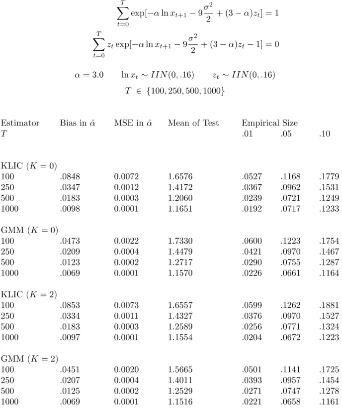
0,2,4,6. Results with automatic bandwidth selection were similar, and so are not shown. Each set is followed by the iterated GMM estimator using the matching lag length. As mentioned earlier, the Newey-West bandwith is equal to the the degree of smoothing in KLIC estimation, so that the estimators can be compared fairly. The first column shows the average bias ˆα−α, which is positive for all experiments, and falls as T rises. GMM yields smaller bias than do the KLIC estimators, at each sample size. The second column gives the mean-squared error in estimating α. Again this is smaller for GMM, at each sample size and degree of smoothing.

The third column gives the mean of the test statistic based on the overidentifying restriction. For GMM this is the usual J-test statistic while for KLIC it is the J K -statistic (10) proposed by Kitamura and Stutzer. With one restriction, the mean of the

χ2(1) tests should be 1 for both test statistics in large samples. All the sample means here exceed one, reflecting the well-known tendency for the J-test to over-reject in small samples. The remaining columns provide further information on this tendency, by giving the empirical sizes of the tests at nominal sizes of 1, 5, and 10 percent.

The comparison of GMM and KLIC test means or sizes shows that KLIC estimation does not solve the over-rejection problem. The KLIC test statistic has a mean very close to that of the J-test statistic, for each sample size and degree of smoothing, except when the estimator adopts a high degree of smoothing with a short sample. As this laboratory environment has no dependence, Table 1 also shows the effects of smoothing when it is not necessary. Here the conclusion is that, provided the ratioT /K is large enough, smoothing does not hurt the finite-sample properties of KLIC estimators or tests, even when there is no persistence in the underlying moments.

Figure 1 provides graphical information on test size, using the P value discrepancy plots described by Davidson and MacKinnon (1998). These are based on the empirical density function (EDF) of the P values, p_r, from R replications. This EDF is is defined as: ˆ F(s_i) = 1 R R r=1 I(p_r ≤s_i) (20)

for s_i ∈(0,1) and whereI is the indicator function taking the value 1 if its argument holds and zero otherwise. The figure shows the discrepancy between empirical size and nominal size, ˆF(s_i)− s_i, graphed against nominal size s_i. The horizontal line is the 5 percent critical value for the Kolmogorov-Smirnov test. Size discrepancies greater than this value are unlikely to have arisen from experimental randomness.

Figure 1 shows the discrepancies for the version of the DGP with i.i.d. data, at T = 250. The tests studied are J and J K (each with smoothing of 0 or 6 lags) and the LM

test. The degree of smoothing is shown in brackets in the figure. TheP value discrepancies for the twoJ-tests are shown in bold as a benchmark. Clearly theLM test is the superior choice at sizes of practical interest, as Imbens, Spady, and Johnson (1998) found. Among the other four tests, the J-tests generally have the smallest distortions at T = 250. We also found that the J K-tests had the smallest distortions once T = 500. By that sample size, though, many of the size discrepancies are not significant.

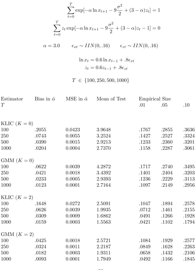
Table 2 studies the version of the simulation model with dependent data. Again the conclusion is that iterated GMM yields less bias and smaller mean-squared errors than than KLIC estimation. Not until the sample size is 1000 do the smoothed KLIC estimators resemble the GMM estimators, to which they are asymptotically equivalent. As for the properties of tests, Table 2 shows that smoothing is necessary to avoid severe over-rejection using either the J or J K test. In conjunction with Table 1, this finding suggests that smoothing should be used in any macroeconomic application where the moments may have persistence, provided that T /K is relatively large.

Figure 2 gives P value discrepancy plots for the DGP with dependent data. Here the P value discrepancies are much larger, as all tests over-reject more strongly. The vertical scale is quite different from that of Figure 1. Figure 2 illustrates the importance of smoothing. While the smoothed J and J K tests have size distortions, they are clearly much better than the tests which do not allow for dependence.

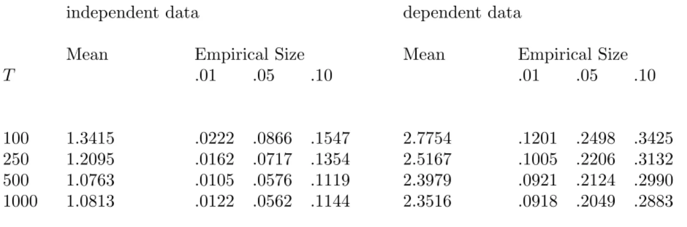
Table 3 summarizes evidence on the LM test (12) proposed by Imbens, Spady, and Johnson. For the i.i.d. DGP (Table 1) this test is better sized than the J-test, as those authors found in the same experiment. For the dependent-data DGP (Table 2) though,

the LM test greatly over-rejects (because it has the appropriate distribution only with independent data), while the smoothed J-test and J K-test do not. The smoothed J -test or the J K-test thus seem the best choices for the macroeconomic practitioner who is concerned about test size but agnostic about persistence.

3.3 Power

The same simulation environment may be used to compare the power of the J tests with that of the KLIC-based tests. In the moment conditions (18) we change the 3 to 4 while keepingα= 3, so that the cross-moment restrictions of log normality no longer hold. Tests of the over-identifying restrictions should be able to detect this violation of the null hypothesis. We examined the power of the tests in the case with dependent data, which is the most relevant to macroeconomics. We also considered other departures from the null hypothesis and found results similar to those reported here.

Figure 3 graphs size-power tradeoff curves for theJ-test and theJ K-test (withK = 0 or 6), at the two sample sizesT = 250 and 500. Again properties of the J-tests are shown as dark lines, while the J K-tests are lighter lines. The degree of smoothing had little effect, and so graphs are not labelled with the value of K. The curves are generated by varying the critical value for the test. At each critical value, we measure the proportion of rejections under the null hypothesis (size) and under the alternative hypothesis (power). The horizontal axis shows size, computed for the DGP satisfying the null, while the vertical axis shows adjusted power. Thus the power comparison is adjusted for the greater size-distortion of the unsmoothed tests. A graph value below the 45◦ line indicates a biased test, with size less than power.

The lower lines in Figure 3 show the size-power curves at a sample size of 250. At this sample size the J-test is biased for sizes less than 0.1. The KLIC-based tests clearly have much higher size-adjusted power. They also have similar properties for each degree of smoothing. The upper lines in Figure 3 show the same properties at a larger sample size of 500, where power increases for all tests. Now theJ-test is no longer biased but again it has much less power against this alternative than do the KLIC tests.

We also calculated P value discrepancies and size-power curves for Hall’s (2000) J C -test, though the results are omitted from Figures 1-3 for ease of viewing. In the simulations, the J C-tests had slightly greater size distortions than the comparable J-tests. In turn, their size-adjusted power was greater than that of the J-tests, but less than that of the

J K-tests.

Our finding low power for the J-test is similar to a conclusion of Smith (1999), who studied the finite-sample properties of tests of the Epstein-Zin asset pricing model. He found that the J-test had low size-adjusted power against some economically interesting alternative DGPs. One possible explanation for the low power of GMM-based test statistics is collinearity in moments, which affects the covariance matrix and reduces the precision of estimators. KLIC estimation avoids this problem because this covariance matrix is not used directly in estimators or test statistics. While a lack of power is not typically a problem in macroeconomic applications, the simulation results suggest that KLIC tests, with a size adjustment, may be very useful diagnostics.

4. Macroeconomic Applications

We next study KLIC and GMM estimators in two macroeconomic applications. In each case we estimate the preference parameters of the intertemporal Euler equation char-acterizing the optimal saving decisions of an infinitely-lived, representative agent. The first application studies constant absolute risk aversion (CARA) while the second application studies constant relative risk aversion (CRRA) utility.

4.1 Consumption with CARA Utility

The first application involves estimating preference parameters from consumption data alone. The consumption problem again is to maximize lifetime utility (14) subject to a budget constraint (15). The period utility function is of the CARA form:

u(c_t) = −exp(−αct)

α (21)

where c_t is real consumption and α is the coefficient of absolute risk aversion. CARA utility has several undesirable properties, including admitting negative consumption. But

Caballero (1990) argued that it is consistent with a range of evidence concerning aggregate consumption. Kimball and Mankiw (1989) applied CARA utility in a theoretical study of tax timing. Few studies attempt to estimate α though. We chose this problem because it has an analytical solution, given a linear, Gaussian model of labour income, and because precautionary saving may be an important component of aggregate saving.

The Euler equation from the maximization problem (14) now is:

exp(−αc_t) =E_t1 +r

1 +θ exp(−αct+1). (22)

The ratio (1 + r)/(1 +θ) generally is not identifiable, so we set r = θ. We define the Euler-equation error for use in estimation as:

_t+1 = exp[−α(ct+1−ct)]−1

α , (23)

then estimate α with the sample versions of the moment conditions:

E[_t+1·z_t] = 0, (24)

with instrumentsz_t. The division byαis consistent with theory, since this lies in the infor-mation set. This division rules out the trivial solution α = 0. Ferson and Constantinides (1991) used a similar transformation in estimating parameters of habit persistence.

Real consumption is measured as monthly U.S. consumption expenditure on non-durables and services, in chain-weighted billions of 1992 dollars, seasonally adjusted. The source is CITIBASE gmcnq + gmcsq. As an instrument we use U.S. real personal dispos-able income in chain-weighted billions of 1992 dollars, gmydpq. Both series are seasonally adjusted and expressed in per capita terms by dividing by population, p16. The sample runs from January 1959 to June 1998, giving 474 observations.

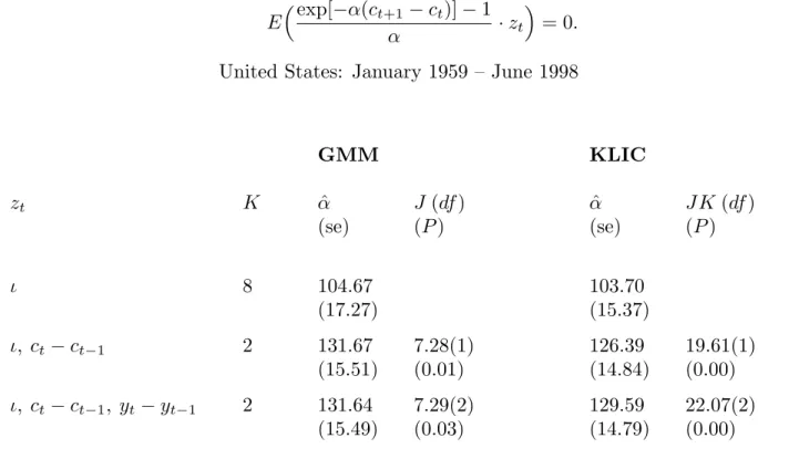
The left side of Table 4 contains iterated GMM estimates of the coefficient of ab-solute risk aversion, α. While various fixed bandwidths were applied, we present only the results based on Newey and West’s (1994) automatic procedure, without prewhiten-ing. We consider three different sets of instruments: z_t = {ι}, z_t = {ι, c_t −c_t−1}, and

z_t ={ι, c_t−c_t−1, y_t−y_t−1}, whereι is a vector of ones. These sets correspond to the cases with exact identification, one overidentifying restriction, and two overidentifying restric-tions respectively. In the first case the Newey-West procedure sets K = T13 = 8 while in the other two cases it gave K = 2. The preference parameter is estimated quite precisely, though the over-identifying restrictions are rejected at conventional significance levels. The implied average coefficients of relative risk aversion are found by multiplying by mean con-sumption, and range from 167 to 209, depending on the instrument set. As in numerous other studies, the elasticity of intertemporal substitution is thus very low. Notice that α

is identified even when z_t contains only a constant, showing that the preference parameter can be estimated even when consumption changes are unpredictable.

The right side of Table 4 contains the corresponding KLIC estimates. The bandwidth

K for smoothing moments is set equal to the Newey-West lag length, as in the Monte Carlo experiments. In this application there is very little persistence in the moments. The first-order autocorrelation of the moment condition, evaluated at the iterated GMM estimates, ranges from -0.10 to 0.04, depending on the instrumentz_t. Thus the choice of K does not have a large effect, as was the case in the i.i.d. simulation environment studied in section 3. The J K test statistic (10) used to assess the overidentifying restrictions rejects them more decisively than does the J test.

The main economic finding is that the KLIC estimators find risk aversion measures similar to those found by GMM. Moreover, the overidentifying restrictions are rejected with both estimators. In fact, the information-theoretic test rejects more resoundingly than the GMM J-test, just as occurred in the Monte Carlo experiments. The table shows asymptotic P values in brackets. We also approximated P values (for the case with one over-identifying restriction) using the i.i.d. version of the simulation model in section 3, with T = 500, and again found very low values.

The light line in Figure 4 shows the Euler equation residuals, exp[−αˆ(c_t+1−c_t)]−1 evaluated at the KLIC estimate with three instruments shown in Table 4. Two other residuals, corresponding to the instruments Δc_t and Δy_t, are not shown here, but of course also play roles in determining the weights on each observation. The KLIC weights,

{ωˆ_t}, are shown as the dark line. They are multiplied by T so as to fit on the same scale as the residuals. The weights clearly are are highly variable over time, dipping down near zero at several observations with large Euler equation residuals. This variation is consistent with the rejection of the overidentifying restrictions. Several observations are essentially omitted in calculating the moments, while several others are over-weighted by more than 100 percent relative to their weights in GMM, which are 1 at this scale. The weights provide a useful, graphical diagnostic when there are multiple instruments and moment conditions.

The data set in this application, with 474 monthly observations, is quite large by the standards of macroeconomics. Even so, there are some differences between the GMM and KLIC estimates and tests in Table 4. We next explore the differences in a second application, with quarterly data.

4.2 CRRA Asset-Pricing

Our second application assumes that period utility is of the power or CRRA form, with parameter α:

u(c_t) = c 1−α t

1−α, (25)

or log utility if α = 1. Asset-pricing with this utility function was the setting for Monte Carlo studies of GMM by Tauchen (1986), Kocherlakota (1990), Hansen, Heaton, and Yaron (1996) and Hansen and Singleton (1996). Again let x be the gross growth rate of consumption and π be the gross growth rate of the corresponding deflator. R_i denotes the gross, nominal yield on a discount bond of maturity i. For one-period and two-period bonds these yields are given by:

1 R_1t = 1 1 +θEt x−α_t+1 π_t+1 1 R2_2t = 1 1 +θ 2 E_t x −α t+1x−αt+2 π_t+1π_t+2 (26)

which exploits the fact that the nominal yields are known at time t.

In this application t counts quarters. R₁ and R₂ are the yields on Canadian three-month and six-three-month treasury bills. The yield data are from CANSIM, seriesb14060 and

b14061and are averages of monthly series. The consumption series is per capita, quarterly, consumption expenditure excluding durables, seasonally adjusted in 1992 dollars: (d15372

- d15373)/d1. The corresponding deflator, used to measure the inflation rate, is the CPI, seriesp100000. The sample includes 104 observations, from 1974 to 1999. We also studied the U.S. data set examined by Hansen, Heaton, and Yaron (1996) but we found a global optimum at unreasonably high risk aversion, as they did.

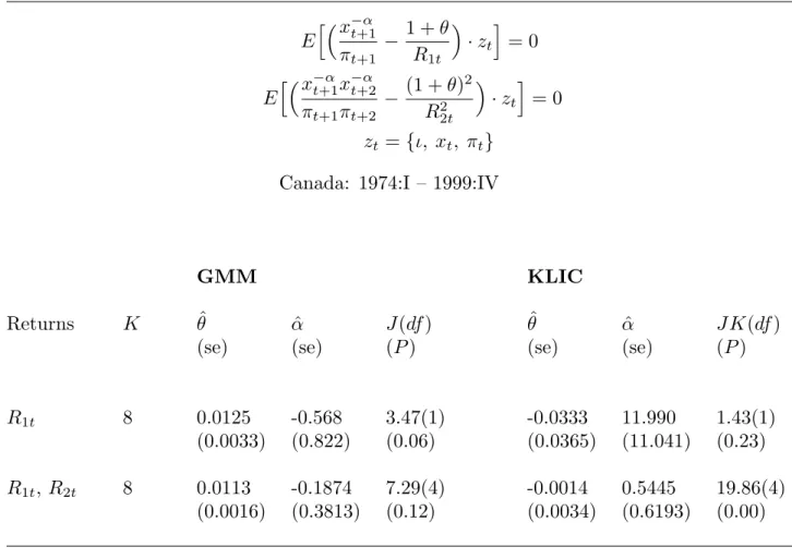
Table 5 contains GMM and KLIC estimates of the preferences parameters α and θ, with K = 8 determined automatically. The instrument set is z_t = {ι, x_t, π_t}. On the left side of the table, GMM finds a significant, positive discount rate of roughly 5% at annual rates. Meanwhile, estimates of α, the coefficient of relative risk aversion, are negative and insignificant, whether estimation uses one yield or two. The J-test does not reject the over-identifying restrictions, at conventional significance levels. Results were very similar with alternate sets of instruments.

KLIC estimation, on the right side of Table 5, yields larger estimates ofα but smaller estimates of θ than GMM does. Both are insignificant. The J K test yields a rejection when two returns are used.

At the iterated GMM estimates (using two asset yields), the first-order autocorrelation coefficient for each moment condition is 0.6. These autocorrelations are not sensitive to the instrument setz_t. Thus this problem resembles the simulation environment with dependent data studied in section 3. As one would expect then, the LM test statistics (not shown) are much larger than the correspondingJ-test statistics. Again the table shows asymptotic

P values in brackets. In the first row of the table, with one over-identifying restriction, we also approximated P values by Monte Carlo methods using the dependent-data version of the simulation model of section 3, with T = 100. In each case, these were larger than the asymptotic values shown, as one would expect.

We also inspected Euler equation residuals and weights from KLIC estimation with two asset returns. As in the previous application, there is a great deal of variation over time. Residuals from the Euler equations are largest when the nominal yields spike in the early 1980s and again in the early 1990s. The weights have a striking pattern: data from

the 1980s are much more consistent with the power-utility CCAPM than are data from the 1990s. Again the weights are a complement to presenting multiple Euler equation residuals and their cross-products with instruments.

5. Summary

KLIC estimation has been proposed by Kitamura and Stutzer (1997) and Imbens, Spady, and Johnson (1998) as an alternative to GMM estimation. This paper has com-pared the two estimation strategies in the task of estimating preference parameters from macroeconomic data. We compared iterated GMM estimators to KLIC estimators with comparable degrees of smoothing. The comparison took place in applications and in sim-ulations.

KLIC estimation provides helpful diagnostics in the form of estimated weights on each observation, but it is computationally somewhat more demanding than GMM. In simula-tions the KLIC estimators had greater bias and mean-squared error than the comparable iterated GMM estimator. Tests arising in KLIC estimation do not appear to provide a so-lution to the problem of over-rejection familiar in GMM estimation and testing. However, KLIC-based tests had size-adjusted power superior to that of the J-test in simulations. Bootstrap corrections along the lines suggested for GMM by Hall and Horowitz (1996) might also be helpful in reducing the size distortions in KLIC estimation.

References

Altonji, J.G. and L.M. Segal, 1996, Small-sample bias in GMM estimation of covariance structures, Journal of Business and Economic Statistics 14, 353-366.

Caballero, R.J., 1990, Consumption puzzles and precautionary savings, Journal of Mone-tary Economics 25, 113-136.

Csisz´ar, I., 1975,I-divergence geometry of probability distributions and minimization prob-lems, Annals of Probability 3, 146-158.

Davidson, R. and MacKinnon, J., 1998, Graphical methods for investigating the size and power of hypothesis tests, Manchester School 66, 1-26.

Ferson, W.E. and G.M. Constantinides, 1991, Habit persistence and durability in aggregate consumption, Journal of Financial Economics 29, 199-240.

Golan, A., G. Judge, and D. Miller, 1996, Maximum entropy econometrics, (Wiley, New York).

Hall, A.R., 2000, Covariance matrix estimation and the power of the overidentifying re-strictions test. Econometrica 68, 1517-1527.

Hall, P. and J. Horowitz, 1996, Bootstrap critical values for tests based on generalized-method-of-moments estimators, Econometrica 64, 891-916.

Hansen, L.P., 1982, Large sample properties of generalized method of moments estimators, Econometrica 50, 1029-1054.

Hansen, L.P. and K.J. Singleton, 1982, Generalized instrumental variables estimation of nonlinear rational expectations models, Econometrica 50, 1269-1286.

Hansen, L.P. and K.J. Singleton, 1996, Efficient estimation of linear asset-pricing models with moving average errors, Journal of Business and Economic Statistics 14, 53-68. Hansen, L.P., J. Heaton and A. Yaron, 1996, Finite-sample properties of some alternative

GMM estimators, Journal of Business and Economic Statistics 14, 262-280.

Imbens, G.W., R.H. Spady and P. Johnson, 1998, Information theoretic approaches to inference in moment condition models, Econometrica 66, 333-357.

Kimball, M.S. and N.G. Mankiw, 1989, Precautionary saving and the timing of taxes, Journal of Political Economy 97, 863-879.

Kitamura, Y. and M. Stutzer, 1997, An information-theoretic alternative to generalized method of moments estimation, Econometrica 65, 861-874.

Kocherlakota, N., 1990, On tests of representative consumer asset pricing models, Journal of Monetary Economics 25, 43-48.

Kullback, S. and R.A. Leibler, 1951, On information and sufficiency, Annals of Mathemat-ical Statistics 22, 79-86.

Newey, W.K. and K.D. West, 1987, A simple, positive semidefinite, heteroskedastic and autocorrelation consistent covariance matrix, Econometrica 55, 703-708.

Newey, W.K. and K.D. West, 1994, Automatic lag selection in covariance matrix estima-tion, Review of Economic Studies 61, 631-654.

Owen, A., 1990, Empirical likelihood ratio confidence regions, Annals of Statistics 18, 90-120.

Owen, A., 1997, Empirical Likelihood, in Encyclopedia of Statistical Sciences. update volume 1. (Wiley, New York).

Qin, J. and J. Lawless, 1994, Empirical likelihood and general estimating equations, Annals of Statistics 22, 300-325.

Smith, D.C., 1999, Finite-sample properties of tests of the Epstein-Zin asset pricing model, Journal of Econometrics 93, 113-148.

Smith, R., 2000, Generalized empirical likelihood criteria for generalized method of mo-ments estimation and inference. mimeo, Department of Economics, University of Bristol.

Stock, J.H. and J.H. Wright, 2000, GMM with weak identification, Econometrica 68, 1055-1096.

Tauchen, G., 1986, Statistical properties of generalized method-of-moment estimators of structural parameters obtained from financial market data, Journal of Business and Economic Statistics 4, 397-416.

Zellner, A., 1997, The Bayesian method of moments: theory and applications, Advances in Econometrics 12, 85-105.

Table 1: Monte Carlo Evidence (i.i.d. data) T t=0 exp[−αlnx_t+1 −9σ 2 2 + (3−α)zt] = 1 T t=0 z_texp[−αlnx_t+1−9σ 2 2 + (3−α)zt −1] = 0 α= 3.0 lnx_t ∼IIN(0, .16) z_t ∼IIN(0, .16) T ∈ {100,250,500,1000}

Estimator Bias in ˆα MSE in ˆα Mean of Test Empirical Size

T .01 .05 .10 KLIC (K = 0) 100 .0848 0.0072 1.6576 .0527 .1168 .1779 250 .0347 0.0012 1.4172 .0367 .0962 .1531 500 .0183 0.0003 1.2060 .0239 .0721 .1249 1000 .0098 0.0001 1.1651 .0192 .0717 .1233 GMM (K = 0) 100 .0473 0.0022 1.7330 .0600 .1223 .1754 250 .0209 0.0004 1.4479 .0421 .0970 .1467 500 .0123 0.0002 1.2717 .0290 .0755 .1287 1000 .0069 0.0001 1.1570 .0226 .0661 .1164 KLIC (K = 2) 100 .0853 0.0073 1.6557 .0599 .1262 .1881 250 .0334 0.0011 1.4327 .0376 .0970 .1527 500 .0183 0.0003 1.2589 .0256 .0771 .1324 1000 .0097 0.0001 1.1554 .0204 .0672 .1223 GMM (K = 2) 100 .0451 0.0020 1.5665 .0501 .1141 .1725 250 .0207 0.0004 1.4011 .0393 .0957 .1454 500 .0125 0.0002 1.2529 .0271 .0747 .1278 1000 .0069 0.0001 1.1516 .0221 .0658 .1161

KLIC (K = 4) 100 .0874 0.0077 2.1170 .0658 .1327 .1957 250 .0342 0.0012 1.4808 .0408 .1011 .1559 500 .0184 0.0003 1.2803 .0263 .0786 .1331 1000 .0096 0.0001 1.1641 .0209 .0675 .1226 GMM (K = 4) 100 .0458 0.0021 1.4606 .0400 .1088 .1679 250 .0207 0.0004 1.3649 .0377 .0938 .1448 500 .0125 0.0002 1.2396 .0256 .0740 .1267 1000 .0069 0.0001 1.1476 .0218 .0649 .1161 KLIC (K = 6) 100 .0825 0.0068 3.3672 .0755 .1456 .2050 250 .0349 0.0012 1.6039 .0442 .1059 .1615 500 .0185 0.0003 1.3044 .0282 .0800 .1362 1000 .0096 0.0001 1.1736 .0216 .0681 .1240 GMM (K = 6) 100 .0468 0.0022 1.3827 .0305 .1007 .1644 250 .0209 0.0004 1.3332 .0352 .0908 .1429 500 .0125 0.0002 1.2267 .0247 .0729 .1251 1000 .0069 0.0001 1.1432 .0213 .0649 .1161

Notes: α is the coefficient of relative risk aversion in the simulation model, K is the bandwidth in KLIC estimation and the Newey-West lag length in GMM estimation. The test statistic follows an asymp-totic χ2(1) distribution and so should have a mean of 1. Entries labelled .01, .05, and .10 are the actual sizes of the test with these nominal sizes. Empirical test sizes can be compared using binomial standard errors. With 10,000 replications the standard error at size ˆsis.01[ˆs(1−sˆ)]12.

Table 2: Monte Carlo Evidence (dependent data) T t=0 exp[−αlnx_t+1 −9σ 2 2 + (3−α)zt] = 1 T t=0 z_texp[−αlnx_t+1−9σ 2 2 + (3−α)zt −1] = 0 α= 3.0 _xt ∼IIN(0, .16) _zt∼IIN(0, .16) lnx_t = 0.6 lnx_t−1+.8_xt z_t = 0.6z_t−1+.8_zt T ∈ {100,250,500,1000}

Estimator Bias in ˆα MSE in ˆα Mean of Test Empirical Size

T .01 .05 .10 KLIC (K = 0) 100 .2055 0.0423 3.9648 .1767 .2855 .3636 250 .0743 0.0055 3.2524 .1427 .2527 .3324 500 .0390 0.0015 2.9213 .1233 .2360 .3201 1000 .0204 0.0004 2.7370 .1158 .2287 .3061 GMM (K = 0) 100 .0622 0.0039 4.2872 .1717 .2740 .3495 250 .0421 0.0018 3.4392 .1401 .2404 .3203 500 .0233 0.0005 2.9393 .1236 .2229 .3113 1000 .0123 0.0001 2.7164 .1097 .2149 .2956 KLIC (K = 2) 100 .1648 0.0272 2.5091 .1047 .1894 .2578 250 .0626 0.0039 1.9935 .0712 .1461 .2155 500 .0309 0.0009 1.6862 .0491 .1266 .1928 1000 .0159 0.0003 1.5563 .0421 .1102 .1794 GMM (K = 2) 100 .0425 0.0018 2.5721 .1084 .1929 .2577 250 .0324 0.0011 2.2187 .0849 .1628 .2263 500 .0182 0.0003 1.9311 .0658 .1432 .2106 1000 .0093 0.0001 1.7949 .0492 .1166 .1845

KLIC (K = 4) 100 .1540 0.0238 3.4948 .0978 .1814 .2449 250 .0614 0.0038 1.8727 .0651 .1346 .1979 500 .0293 0.0008 1.5551 .0423 .1111 .1757 1000 .0149 0.0002 1.4231 .0358 .0944 .1602 GMM (K = 4) 100 .0449 0.0020 2.0438 .0805 .1663 .2300 250 .0287 0.0008 1.8956 .0691 .1396 .1988 500 .0163 0.0003 1.6686 .0501 .1207 .1815 1000 .0081 0.0001 1.5669 .0451 .1086 .1715 KLIC (K = 6) 100 .1360 0.0185 5.7943 .1069 .1867 .2477 250 .0613 0.0038 1.8719 .0656 .1327 .1964 500 .0288 0.0008 1.5235 .0415 .1062 .1694 1000 .0146 0.0002 1.3817 .0336 .0896 .1529 GMM (K = 6) 100 .0508 0.0026 1.7835 .0605 .1488 .2144 250 .0272 0.0007 1.7255 .0598 .1289 .1861 500 .0154 0.0002 1.5475 .0429 .1104 .1695 1000 .0074 0.0001 1.4643 .0396 .0974 .1585

Notes: α is the coefficient of relative risk aversion in the simulation model, K is the bandwidth in KLIC estimation and the Newey-West lag length in GMM estimation. The test statistic follows an asymp-totic χ2(1) distribution and so should have a mean of 1. Entries labelled .01, .05, and .10 are the actual sizes of the test with these nominal sizes. Empirical test sizes can be compared using binomial standard errors. With 10,000 replications the standard error at size ˆsis.01[ˆs(1−sˆ)]12.

Table 3: Monte Carlo Evidence (LM Test)

independent data dependent data

Mean Empirical Size Mean Empirical Size

T .01 .05 .10 .01 .05 .10

100 1.3415 .0222 .0866 .1547 2.7754 .1201 .2498 .3425

250 1.2095 .0162 .0717 .1354 2.5167 .1005 .2206 .3132

500 1.0763 .0105 .0576 .1119 2.3979 .0921 .2124 .2990

1000 1.0813 .0122 .0562 .1144 2.3516 .0918 .2049 .2883

Notes: The LM test statistic follows an asymptotic χ2(1) distribution when the moments are serially uncorrelated and so should have a mean of 1. Entries labelled .01, .05, and .10 are the actual sizes of the test with these nominal sizes.

Table 4: Estimation of Constant Absolute Risk Aversion (CARA) E _exp[−α(c t+1−ct)]−1 α ·zt = 0.

United States: January 1959 – June 1998

GMM KLIC z_t K αˆ J(df) αˆ J K(df) (se) (P) (se) (P) ι 8 104.67 103.70 (17.27) (15.37) ι, c_t−c_t−1 2 131.67 7.28(1) 126.39 19.61(1) (15.51) (0.01) (14.84) (0.00) ι, c_t−c_t−1, y_t −y_t−1 2 131.64 7.29(2) 129.59 22.07(2) (15.49) (0.03) (14.79) (0.00)

Notes: ιis a vector of ones;cis expenditure on nondurables and services; yis personal disposable income; both time series are real, per capita, monthly, and seasonally adjusted.

Table 5: Estimation of Constant Relative Risk Aversion (CRRA) E _x−α t+1 π_t+1 − 1 +θ R_1t ·z_t = 0 E _x−α t+1x−αt+2 π_t+1π_t+2 − (1 +θ)2 R2_2t ·z_t = 0 z_t ={ι, x_t, π_t}

Canada: 1974:I – 1999:IV

GMM KLIC

Returns K θˆ αˆ J(df) θˆ αˆ J K(df)

(se) (se) (P) (se) (se) (P)

R_1t 8 0.0125 -0.568 3.47(1) -0.0333 11.990 1.43(1)

(0.0033) (0.822) (0.06) (0.0365) (11.041) (0.23)

R_1t, R_2t 8 0.0113 -0.1874 7.29(4) -0.0014 0.5445 19.86(4) (0.0016) (0.3813) (0.12) (0.0034) (0.6193) (0.00)

Notes: ι is a vector of ones; xis the gross growth rate of expenditure on nondurables and services (real, quarterly, seasonally adjusted, per capita);π is the gross cpi inflation rate;R1 is the gross yield on