Consistent Multitask Learning with
Nonlinear Output Relations
Carlo Ciliberto•,1 Alessandro Rudi•,∗,2 Lorenzo Rosasco3,4,5 Massimiliano Pontil1,5 {c.ciliberto,m.pontil}@ucl.ac.uk [email protected] [email protected]
1
Department of Computer Science, University College London, London, UK. 2
INRIA - Sierra Project-team and École Normale Supérieure, Paris, France. 3
Massachusetts Institute of Technology, Cambridge, USA. 4
Università degli studi di Genova, Genova, Italy. 5
Istituto Italiano di Tecnologia, Genova, Italy. •Equal Contribution
Abstract
Key to multitask learning is exploiting the relationships between different tasks in order to improve prediction performance. Most previous methods have focused on the case where tasks relations can be modeled as linear operators and regularization approaches can be used successfully. However, in practice assuming the tasks to be linearly related is often restrictive, and allowing for nonlinear structures is a challenge. In this paper, we tackle this issue by casting the problem within the framework of structured prediction. Our main contribution is a novel algorithm for learning multiple tasks which are related by a system of nonlinear equations that their joint outputs need to satisfy. We show that our algorithm can be efficiently implemented and study its generalization properties, proving universal consistency and learning rates. Our theoretical analysis highlights the benefits of non-linear multitask learning over learning the tasks independently. Encouraging experimental results show the benefits of the proposed method in practice.
1
Introduction
Improving the efficiency of learning from human supervision is one of the great challenges in machine learning. Multitask learning is one of the key approaches in this sense and it is based on the assumption that different learning problems (i.e. tasks) are often related, a property that can be exploited to reduce the amount of data needed to learn each individual tasks and in particular to learn efficiently novel tasks (a.k.a. transfer learning, learning to learn [1]). Special cases of multitask learning include vector-valued regression and multi-category classification; applications are numerous, including classic ones in geophysics, recommender systems, co-kriging or collaborative filtering (see [2, 3, 4] and references therein). Diverse methods have been proposed to tackle this problem, for examples based on kernel methods [5], sparsity approaches [3] or neural networks [6]. Furthermore, recent theoretical results allowed to quantify the benefits of multitask learning from a generalization point view when considering specific methods [7, 8].
A common challenge for multitask learning approaches is the problem of incorporating prior as-sumptions on the task relatedness in the learning process. This can be done implicitly, as in neural networks [6], or explicitly, as done in regularization methods by designing suitable regularizers [5]. This latter approach is flexible enough to incorporate different notions of tasks’ relatedness expressed, for example, in terms of clusters or a graph, see e.g. [9, 10]. Further, it can be extended tolearnthe tasks’ structures when they are unknown [3, 11, 12, 13, 14, 15, 16]. However, most
∗
Work performed while A.R. was at the Istituto Italiano di Tecnologia.
regularization approaches are currently limited to imposing, or learning, tasks structures expressed by linear relations (see Sec.5). For example an adjacency matrix in the case of graphs or a block matrix in the case of clusters. Clearly while such a restriction might make the problem more amenable to statistical and computational analysis, in practice it might be a severe limitation.
Encoding and exploitingnonlineartask relatedness is the problem we consider in this paper. Previous literature on the topic is scarce. Neural networks naturally allow to learn with nonlinear relations, however it is unclear whether such relations can be imposed a-priori. As explained below, our problem has some connections to that of manifold valued regression [17]. To our knowledge this is the first work addressing the problem of explicitly imposing nonlinear output relations among multiple tasks. Close to our perspective is [18], where however a different approach is proposed, implicitly enforcing a nonlinear structure on the problem by requiring the parameters of each task predictors to lie on a shared manifold in the hypotheses space.
Our main contribution is a novel method for learning multiple tasks which arenonlinearlyrelated. We address this problem from the perspective of structured prediction (see [19, 20] and references therein) building upon ideas recently proposed in [21]. Specifically we look at multitask learning as the problem of learning a vector-valued function taking values in a prescribed set, which models tasks’ interactions. We also discuss how to deal with possible violations of such a constraint set. We study the generalization properties of the proposed approach, proving universal consistency and learning rates. Our theoretical analysis allows also to identify specific training regimes in which multitask learning is clearly beneficial in contrast to learning all tasks independently.
2
Problem Formulation
Multitask learning (MTL) studies the problem of estimating multiple (real-valued) functions
f1, . . . , fT :X →R (1)
from corresponding training sets(xit, yit)ni=1t withxit∈ Xandyit∈R, fort= 1, . . . , T. The key
idea in MTL is to estimatef1, . . . , fT jointly, rather than independently. The intuition is thatifthe
different tasks arerelatedthis strategy can lead to a substantial decrease of sample complexity, that is the amount of data needed to achieve a given accuracy. The crucial question is then how to encode and exploit such relations among the tasks.
Previous work on MTL has mostly focused on studying the case where the tasks are linearly related (see Sec.5). Indeed, this allows to capture a wide range of relevant situations and the resulting problem can be often cast as a convex optimization, which can be solved efficiently. However, it is not hard to imagine situations where different tasks might be nonlinearly related. As a simple example consider the problem of learning two functionsf1, f2: [0,2π]→R, withf1(x) = cos(x)
andf2(x) = sin(x). Clearly the two tasks are strongly related one to the other (they need to satisfy f1(x)2+f2(x)2−1 = 0for allx∈[0,2π]) but such structure in nonlinear (here an equation of
degree2). More realistic examples can be found for instance in the context of modeling physical systems, such as the case of a robot manipulator. A prototypical learning problem (see e.g. [22]) is to associate the current state of the system (position, velocity, acceleration) to a variety of measurements (e.g. torques) that are nonlinearly related one to the other by physical constraints (see e.g. [23]). Following the intuition above, in this work we model tasks relations as a set ofPequations. Specifi-cally we consider aconstraint functionγ:RT →
RPand require thatγ(f1(x), . . . , fT(x)) = 0for
allx∈ X. Whenγis linear, the problem reverts to linear MTL and can be addressed via standard approaches (see Sec.5). On the contrary, the nonlinear case becomes significantly more challenging and it is not clear how to address it in general. The starting point of our study is to consider the tasks predictors as a vector-valued functionf = (f1, . . . , fT) :X →RT but then observe thatγ
imposes constraints on its range. Specifically, in this work we restrictf :X → Cto take values in theconstraint set
C=
y∈RT |γ(y) = 0 ⊆ RT (2)
and formulate the nonlinear multitask learning problem as that of finding a good approximation b
f :X → Cto the solution of the multi-taskexpected riskminimization problem
minimize f:X →C E(f), E(f) = 1 T T X t=1 Z X ×R `(ft(x), y)dρt(x, y) (3)
where`:R×R→Ris a prescribed loss function measuring prediction errors for each individual
task and, for everyt = 1, . . . , T,ρtis the distribution onX ×Rfrom which the training points (xit, yit)ni=1t have been independently sampled.
Nonlinear MTL poses several challenges to standard machine learning approaches. Indeed, whenC
is a linear space (e.g.γis a linear map) the typical strategy to tackle problem (3) is to minimize the empirical riskT1PT
t=1 1 nt
Pnt
i=1`(ft(xit), yit)over some suitable space of hypothesesf :X → C
within which optimization can be performed efficiently. However, if C is a nonlinear subset of
RT, it is not clear how to parametrize a “good” space of functions since most basic properties
typically needed by optimization algorithms are lost (e.g.f1, f2:X → Cdoes not necessarily imply
f1+f2:X → C). To address this issue, in this paper we adopt thestructured predictionperspective
proposed in [21], which we review in the following.
2.1 Background: Structured Prediction and the SELF Framework
The term structured prediction typically refers to supervised learning problems with discrete outputs, such as strings or graphs [19, 20, 24]. The framework in [21] generalizes this perspective to account for a more flexible formulation of structured prediction where the goal is to learn an estimator approximating the minimizer of
minimize f:X →C
Z
X ×Y
L(f(x), y)dρ(x, y) (4) given a training set(xi, yi)ni=1of points independently sampled from an unknown distributionρon X × Y, whereL:Y × Y →Ris a loss function. The output setsY andC ⊆ Yare not assumed
to be linear spaces but can be either discrete (e.g. strings, graphs, etc.) or dense (e.g. manifolds, distributions, etc.) sets of “structured” objects. This generalization will be key to tackle the question of multitask learning with nonlinear output relations in Sec.3since it allows to consider the case whereCis a generic subset ofY=RT. The analysis in [21] hinges on the assumption that the lossL
is “bi-linearizable”, namely
Definition 1(SELF). LetYbe a compact set. A function`:Y × Y →Ris aStructure Encoding
Loss Function (SELF)if there exists a continuous feature mapψ:Y → H, withHa reproducing kernel Hilbert space onYand a continuous linear operatorV :H → Hsuch that for ally, y0∈ Y
`(y, y0) =hψ(y), V ψ(y0)iH. (5)
In the original work the SELF definition was dubbed “loss trick” as a parallel to thekernel trick[25]. As we discuss in Sec.4, most MTL loss functions indeed satisfy the SELF property. Under this assumption, it can be shown that a solutionf∗:X → Cto Eq. (4) must satisfy
f∗(x) = argmin c∈C hψ(c), V g∗(x)iH with g∗(x) = Z Y ψ(y)dρ(y|x) (6) for allx∈ X (see [21] or the Appendix). Sinceg∗ :X → His a function with values in a linear space, we can apply standard regression techniques to learn abg:X → Hto approximateg∗given
(xi, ψ(yi))ni=1and then obtain the estimatorfb:X → Cas b
f(x) = argmin c∈C
hψ(c), V bg(x)iH ∀x∈ X. (7)
The intuition here is that ifbgis close tog∗, so it will be
b
f tof∗(see Sec.4for a rigorous analysis of
this relation). Ifbgis thekernel ridge regressionestimator obtained by minimizing the empirical risk
1 n
Pn
i=1kg(xi)−ψ(yi)k2H(plus regularization), Eq. (7) becomes
b f(x) = argmin c∈C n X i=1 αi(x)L(c, yi), α(x) = (α1(x), . . . , αn(x))>= (K+nλI)−1Kx (8)
sincebgcan be written as the linear combinationbg(x) =Pn
i=1αi(x)ψ(yi)and the loss functionLis
SELF. In the above formulaλ >0is a hyperparameter,I∈Rn×nthe identity matrix,K∈Rn×n
the kernel matrix with elementsKij =k(xi, xj),Kx∈Rnthe vector with entries(Kx)i=k(x, xi)
The SELF structured prediction approach is therefore conceptually divided into two distinct phases: alearningstep, where the score functionsαi:X →Rare estimated, which consists in solving the
kernel ridge regression inbg, followed by apredictionstep, where the vectorc∈ Cminimizing the weighted sum in Eq. (8) is identified. Interestingly, while the feature mapψ, the spaceHand the operatorV allow to derive the SELF estimator,their knowledge is not needed to evaluatefb(x)in practicesince the optimization at Eq. (8) depends exclusively on the lossLand the score functions αi.
3
Structured Prediction for Nonlinear MTL
In this section we present the main contribution of this work, namely the extension of the SELF framework to the MTL setting. Furthermore, we discuss how to cope with possible violations of the constraint set in practice. We study the theoretical properties of the proposed estimator in Sec.4. We begin our analysis by applying the SELF approach to vector-valued regression which will then lead to the MTL formulation.
3.1 Nonlinear Vector-valued Regression
Vector-valued regression (VVR) is a special instance of MTL where for each input, all output examples are available during training. In other words, the training sets can be combined into a single dataset(xi, yi)in=1, withyi= (yi1, . . . , yit)>∈RT. If we denoteL:RT ×RT →Rthe separable
lossL(y, y0) =T1P
t=1`(yt, y 0
t), nonlinear VVR coincides with the structured prediction problem
in Eq. (4). IfLis SELF, we can therefore obtain an estimator according to Eq. (8).
Example 1(Nonlinear VVR with Square Loss). LetL(y, y0) =PT
t=1(yt−yt0)2. Then, the SELF
estimator for nonlinear VVR can be obtained asfb:X → Cfrom Eq. (8) and corresponds to the projection ontoC b f(x) = argmin c∈C kc−b(x)/a(x)k22= ΠC(b(x)/a(x)) (9) with a(x) = Pn i=1αi(x)andb(x) = P n i=1αi(x)yi. Interestingly, b(x) = P n i=1αi(x)yi =
Y>(K+nλI)−1Kxcorresponds to the solution of the standard vector-valued kernel ridge regression
withoutconstraints (we denotedY ∈Rn×T the matrix with rowsyi>). Therefore, nonlinear VVR
consists in:1)computing theunconstrainedkernel ridge regression estimatorb(x),2)normalizing it bya(x)and3)projecting it ontoC.
The example above shows that for specific loss functions the estimation offb(x)can be significantly simplified. In general, such optimization will depend on the properties of the constraint setC(e.g. convex, connected, etc.) and the loss`(e.g. convex, smooth, etc.). In practice, ifC is a discrete (or discretized) subset ofRT, the computation can be performed efficiently via a nearest neighbor
search (e.g. usingk-d treesbased approaches to speed up computations [26]). IfCis a manifold, recentgeometric optimizationmethods [27] (e.g. SVRG [28]) can be applied to find critical points of Eq. (8). This setting suggests a connection with manifold regression as discussed below.
Remark 1(Connection to Manifold Regression). WhenCis a Riemannian manifold, the problem of learningf :X → Cshares some similarities to themanifold regressionsetting studied in [17] (see also [29] and references therein). Manifold regression can be interpreted as a vector-valued learning setting where outputs are constrained to be inC ⊆RT and prediction errors are measured according
to thegeodesic distance. However, note that the two problems are also significantly different since,
1)in MTL noise could make output examplesyilie close but not exactly on the constraint setCand
moreover,2)the loss functions used in MTL typically measure errors independently for each task (as in Eq. (3), see also [5]) and rarely coincide with a geodesic distance.
3.2 Nonlinear Multitask Learning
Differently from nonlinear vector-valued regression, the SELF approach introduced in Sec.2.1cannot be applied to the MTL setting. Indeed, the estimator at Eq. (8) requires knowledge of all tasks outputs yi∈ Y =RT for every training inputxi∈ X while in MTL we have a separate dataset(xit, yit)ni=1t
Therefore, in this work we extend the SELF framework to nonlinear MTL. We begin by proving a characterization of the minimizerf∗:X → Cof the expected riskE(f)akin to Eq. (6).
Proposition 2. Let`:R×R→Rbe SELF, with`(y, y0) =hψ(y), V ψ(y0)iH. Then, the expected
riskE(f)introduced at Eq. (3) admits a measurable minimizerf∗ :X → C. Moreover, any such minimizer satisfies, almost everywhere onX,
f∗(x) = argmin c∈C T X t=1 hψ(ct), V g∗t(x)iH, with gt∗(x) = Z R ψ(y)dρt(y|x). (10)
Prop. 2extends Eq. (6) by relying on the linearity induced by the SELF assumption combined with theAumann’s principle[30], which guarantees the existence of a measurable selectorf∗for the minimization problem at Eq. (10) (see Appendix). By following the strategy outlined in Sec.2.1, we propose to learnTindependent functionsbgt:X → H, each aiming to approximate the corresponding
gt∗:X → Hand then definefb:X → Csuch that
b f(x) = argmin c∈C T X t=1 hψ(ct), V bgt(x)iH ∀x∈ X. (11)
We choose thebgtto be the solutions toT independent kernel ridge regressions problems
minimize g∈H⊗G 1 nt nt X i=1 kg(xit)−ψ(yit)k2+λtkgk2H⊗G (12)
for t = 1, . . . , T, where G is a reproducing kernel Hilbert space on X associated to a kernel k:X × X →Rand the candidate solutiong:X → His an element ofH ⊗ G. The following result
shows that in this setting, evaluating the estimatorfbcan be significantly simplified.
Proposition 3(The Nonlinear MTL Estimator). Letk:X × X →Rbe a reproducing kernel with
associated reproducing kernel Hilbert spaceG. Letbgt :X → Hbe the solution of Eq. (12) for
t= 1, . . . , T. Then the estimatorfb:X → Cdefined at Eq. (11) is such that
b f(x) = argmin c∈C T X t=1 nt X i=1 αit(x)`(ct, yit), (α1t(x), . . . , αntt(x)) >= (K t+ntλtI)−1Ktx (13)
for allx ∈ X andt = 1, . . . , T, whereKt ∈ Rnt×nt denotes the kernel matrix of thet-th task,
namely(Kt)ij =k(xit, xjt), andKtx∈Rntthe vector withi-th component equal tok(x, x
it). Prop. 3provides an equivalent characterization for nonlinear MTL estimator at Eq. (11) that is more amenable to computations (it does not require explicit knowledge ofH,ψorV) and generalizes the SELF approach (indeed for VVR, Eq. (13) reduces to the SELF estimator at Eq. (8)). Interestingly, the proposed strategy learns the score functionsαim : X →Rseparately for each task and then
combines them in the joint minimization overC. This can be interpreted as the estimator weighting predictions according to how “reliable” each task is on the inputx∈ X. We make this intuition more clear in the following.
Example 2(Nonlinear MTL with Square Loss). Let`be the square loss. Then, analogously to Example 1we have that for anyx∈ X, the multitask estimator at Eq. (13) is
b f(x) = argmin c∈C T X t=1 at(x) ct−bt(x)/at(x) 2 (14) withat(x) = P nt i=1αit(x)andbt(x) = P nt
i=1αit(x)yit, which corresponds to perform the
pro-jectionfb(x) = ΠCA(x)(w(x))of the vectorw(x) = (b1(x)/a1(x), . . . , bT(x)/aT(x))according to
the metric deformation induced by the matrixA(x) = diag(a1(x), . . . , aT(x)). This suggests to
interpretat(x)as a measure of confidence of tasktwith respect tox∈ X. Indeed, tasks with small
3.3 Extensions: ViolatingC
In practice, it is natural to expect the knowledge of the constraints setCto be not exact, for instance due to noise or modeling inaccuracies. To address this issue, we consider two extensions of nonlinear MTL that allow candidate predictors to slightly violate the constraintsCand introduce a hyperparameter to control this effect.
Robustness w.r.t. perturbations of C. We soften the effect of the constraint set by requiring candidate predictors to take valuewithina radiusδ >0fromC, namelyf :X → Cδ with
Cδ ={c+r|c∈ C, r∈RT,krk ≤δ}. (15)
The scalarδ >0is now a hyperparameter ranging from0(C0=C) to+∞(C∞=RT).
Penalizing w.r.t. the distance fromC. We can penalize predictions depending on their distance from the setCby introducing a perturbed version`t
µ:RT ×RT →Rof the loss
`tµ(y, z) =`(yt, zt) +kz−ΠC(z)k2/µ for ally, z∈RT (16)
whereΠC :RT → Cdenotes the orthogonal projection ontoC(seeExample 1). Below we report the
closed-from solution for nonlinear vector-valued regression with square loss.
Example 3(VVR and Violations ofC). With the same notation asExample 1, letf0:X → Cdenote
the solution at Eq. (9) of nonlinear VVR withexactconstraints, letr=b(x)/a(x)−f0(x)∈RT. Then,
the solutions to the problem with robust constraintsCδ and perturbed loss functionLµ=T1P
t` t µ
are respectively (see Appendix for the MTL) b
fδ(x) =f0(x) +r min(1, δ/krk) and fbµ(x) =f0(x) +r µ/(1 +µ). (17)
4
Generalization Properties of Nonlinear MTL
We now study the statistical properties of the proposed nonlinear MTL estimator. Interestingly, this will allow to identify specific training regimes in which nonlinear MTL achieves learning rates significantly faster than those available when learning the tasks independently. Our analysis revolves around the assumption that the loss function used to measure prediction errors is SELF. To this end we observe that most multitask loss functions are indeed SELF.
Proposition 4. Let`¯: [a, b] → Rbe differentiable almost everywhere with derivative Lipschitz
continuous almost everywhere. Let ` : [a, b]×[a, b] → R be such that `(y, y0) = ¯`(y−y0)
or `(y, y0) = ¯`(yy0) for all y, y0 ∈ R. Then: (i) ` is SELF and (ii) the separable function L:YT × YT →
Rsuch thatL(y, y0) =T1
PT
t=1`(yt, y 0
t)for ally, y0 ∈ YT is SELF.
Interestingly, most (mono-variate) loss functions used in multitask and supervised learning satisfy the assumptions ofProp. 4. Typical examples are the square loss(y−y0)2, hingemax(0,1−yy0)
or logisticlog(1−exp(−yy0)): the corresponding derivative with respect toz=y−y0orz=yy0 exists and it is Lipschitz almost everywhere on compact sets.
The nonlinear MTL estimator introduced in Sec.3.2relies on the intuition that if for eachx∈ X
the kernel ridge regression solutionsbgt(x)are close to the conditional expectations g∗t(x), then
alsofb(x)will be close tof∗(x). The following result formally characterizes the relation between the two problems, proving what is often referred to as acomparison inequalityin the context of surrogate frameworks [31]. Throughout the rest of this section we assumeρt(x, y) =ρt(y|x)ρX(x)
for eacht= 1, . . . , T and denotekgkL2
ρX theL
2 ρX =L
2(X,H, ρX)norm of a functiong:X → H
according to the marginal distributionρX.
Theorem 5(Comparison Inequality). With the same assumptions ofProp. 2, fort = 1, . . . , T let f∗:X → Candgt∗:X → Hbe defined as in Eq. (10), letbgt:X → Hbe measurable functions
and letfb:X → Csatisfy Eq. (11). LetV∗be the adjoint ofV. Then,
E(fb)− E(f∗)≤qC,`,T v u u t 1 T T X t=1 kbgt−gt∗k2Lρ2 X , qC,`,T = 2 sup c∈C v u u t 1 T T X t=1 kV∗ψ(c t)k2H. (18)
The comparison inequality at Eq. (18) is key to study the generalization properties of our nonlinear MTL estimator by showing that we can control itsexcess riskin terms of how well thebgtapproximate
the truegt∗(see Appendix for a proof ofThm. 5).
Theorem 6. LetC ⊆[a, b]T, letX be a compact set andk:X × X →
Ra continuous universal
reproducing kernel (e.g. Gaussian). Let`: [a, b]×[a, b]→Rbe a SELF. LetfbN :X → Cdenote
the estimator at Eq. (13) withN= (n1, . . . , nT)training points independently sampled fromρtfor
each taskt= 1, . . . , T andλt=n −1/4
t . Letn0= min1≤t≤Tnt. Then, with probability1 lim
n0→+∞
E(fbN) = inf
f:X →CE(f). (19)
The proof ofThm. 6relies on the comparison inequality inThm. 5, which links the excess risk of the MTL estimator to the square error betweenˆgtandg∗t. Standard results from kernel ridge
regression allow to conclude the proof [32] (see a more detailed discussion in the Appendix). By imposing further standard assumptions, we can also obtain generalization bounds onkbgt−g∗tkL2
that automatically apply to nonlinear MTL again via the comparison inequality, as shown below.
Theorem 7. With the same assumptions and notation ofThm. 6letfbN :X → Cdenote the estimator
at Eq. (13) withλt=n−1 /2
t and assumeg∗t ∈ H ⊗ G, for allt= 1, . . . , T. Then for anyτ >0we
have, with probability at least1−8e−τ, that E(fbN)− inf
f:X →CE(f) ≤ qC,`,T h` τ
2 n−1/4
0 logT, (20)
whereqC,`,T is defined as in Eq. (18) andh`is a constant independent ofC, N, nt, λt, τ, T.
The the excess risk bound inThm. 7is comparable to that in [21] (Thm.5). To our knowledge this is the first result studying the generalization properties of a learning approach to MTL with constraints.
4.1 Benefits of Nonlinear MTL
The rates inThm. 7strongly depend on the constraintsCvia the constantqC,`,T. The following result
studies two special cases that allow to appreciate this effect.
Lemma 8. LetB ≥1,B= [−B, B]T,S ⊂
RT be the sphere of radiusBcentered at the origin
and let`be the square loss. ThenqB,`,T ≤2 √
5B2andqS,`,T ≤2 √
5B2T−1/2. To explain the effect ofCon MTL, definen=PT
t=1ntand assume thatn0=nt=n/T.Lemma 8
together with Thm.7shows that when the tasks are assumed not to be related (i.e.C=B) the learning rate of nonlinear MTL is ofOe((Tn)1/4), as if the tasks were learned independently. On the other hand, when the tasks have a relation (e.g.C=S, implying a quadratic relation between the tasks) nonlinear MTL achieves a learning rate ofOe((nT1 )1/4), which improves as the number of tasks increases and as the total number of observed examples increases. Specifically, forT of the same order ofn, we obtain a rate ofOe(n−1/2)which is comparable to the optimal rates available for kernel ridge regression with only one task trained on the total numbernof examples[32]. This observation corresponds to the intuition that if we have many related tasks with few training examples each, we can expect to achieve significantly better generalization by taking advantage of such relations rather than learning each task independently.
5
Connection to Previous Work: Linear MTL
In this work we formulated the nonlinear MTL problem as that of learning a functionf :X → C
taking values in a set of constraintsC ⊆RTimplicitlyidentified by a set of equationsγ(f(x)) = 0. An
alternative approach would be to characterize the setCvia anexplicitparametrizationθ:RQ → C, for
Q∈N, so that the multitask predictor can be decomposed asf =θ◦h, withh:X →RQ. We can
learnh:X →RQusing empirical risk minimization strategies such as Tikhonov regularization,
minimize h=(h1,...,hQ)∈HQ 1 n n X i=1 L(θ◦h(xi), yi) +λ Q X q=1 khqk2H (21)
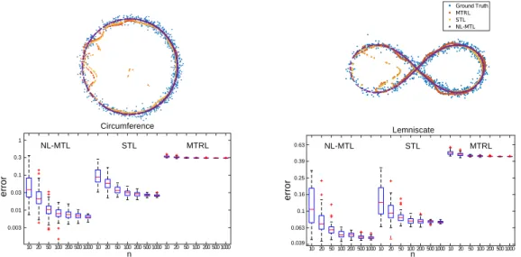
Figure 1: (Bottom) MSE (logaritmic scale) of MTL methods for learning constrained on a circumference (Left) or a Lemniscate (Right). Results are reported in a boxplot across10trials. (Top) Sample predictions of the three methods trained on100points and compared with the ground truth.
since candidatehtake value inRQand thereforeHcan be a standard linear space of hypotheses.
However, while Eq. (21) is interesting from the modeling standpoint, it also poses several problems:
1)θcan be nonlinear or even non-continuous, making Eq. (21) hard to solve in practice even for
Lconvex;2)θis not uniquely identified byC and therefore different parametrizations may lead to very differentfb=θ◦bh, which is not always desirable;3) There are few results on empirical risk minimization applied to generic loss functionsL(θ(·),·)(via so-called oracle inequalities, see [30] and references therein), and it is unclear what generalization properties to expect in this setting. A relevant exception to the issues above is the case where θ is linear. In this setting Eq. (21) becomes more amenable to both computations and statistical analysis and indeed most previous MTL literature has been focused on this setting, either by designing ad-hoc output metrics [33], linear output encodings [34] or regularizers [5]. Specifically, in this latter case the problem is cast as that of minimizing the functional
minimize f=(f1,...,fT)∈HT n X i=1 L(f(xi), yi) +λ T X t,s=1 Atshft, fsiH (22)
where the psd matrix A = (Ats)Ts,t=1 encourages linear relations between the tasks. It can be
shown that this problem is equivalent to Eq. (21) when theθ ∈ RT×Q is linear andAis set to
the pseudoinverse ofθθ>. As shown in [14], a variety of situations are recovered considering the
approach above, such as the case where tasks are centered around a common average [9], clustered in groups [10] or sharing the same subset of features [3, 35]. Interestingly, the above framework can be further extended to estimate the structure matrixAdirectly from data, an idea initially proposed in [12] and further developed in [2, 14, 16].
6
Experiments
Synthetic Dataset. We considered a model of the formy=f∗(x) +, with∼N(0, σI)noise
sam-pled according to a normal distribution andf∗:X → C, whereC ⊂R2was either a circumference or
a lemniscate (see Fig.1) of equationγcirc(y) =y12+y22−1 = 0andγlemn(y) =y41−(y21−y22) = 0
fory∈R2. We setX = [−π, π]andfcirc∗ (x) = (cos(x), sin(x))orflemn∗ (x) = (sin(x), sin(2x))
the parametric functions associated respectively to the circumference and Lemniscate. We sampled from10to1000points for training and1000for testing, with noiseσ= 0.05.
We trained and tested three regression models over10trials. We used a Gaussian kernel on the input and chose the corresponding bandwidth and the regularization parameterλby hold-out cross-validation on30%of the training set (see details in the appendix). Fig.1(Bottom) reports the mean
Table 1: Explained variance of the robust (NL-MTL[R]) and perturbed (NL-MTL[P]) variants of nonlinear MTL, compared with linear MTL methods on the Sarcos dataset reported from [16].
STL MTL[36] CMTL[10] MTRL[11] MTFL[13] FMTL[16] NL-MTL[R] NL-MTL[P]
Expl. 40.5 34.5 33.0 41.6 49.9 50.3 55.4 54.6
Var. (%) ±7.6 ±10.2 ±13.4 ±7.1 ±6.3 ±5.8 ±6.5 ±5.1
Table 2: Rank prediction error according to the weighted binary loss in [37, 21].
NL-MTL SELF[21] Linear[37] Hinge[38] Logistic[39] SVMStruct[20] STL MTRL[11]
Rank 0.271 0.396 0.430 0.432 0.432 0.451 0.581 0.613
Loss ±0.004 ±0.003 ±0.004 ±0.008 ±0.012 ±0.008 0.003 ±0.005
square error (MSE) of our nonlinear MTL approach (NL-MTL) compared with the standard least squares single task learning (STL) baseline and the multitask relations learning (MTRL) from [11], which encourages tasks to belinearlydependent. However, for both circumference and Lemniscate, the tasks are stronglynonlinearlyrelated. As a consequence our approach consistently outperforms its two competitors which assume only linear relations (or none at all). Fig.1(Top) provides a qualitative comparison on the three methods (when trained with100examples) during a single trial.
Sarcos Dataset. We report experiments on the Sarcos dataset [22]. The goal is to predict the torque measured at each joint of a7degrees-of-freedom robotic arm, given the current state, velocities and accelerations measured at each joint (7tasks/torques for21-dimensional input). We used the10
dataset splits available online for the dataset in [13], each containing2000examples per task with15
examples used for training/validation while the rest is used to measure errors in terms of theexplained variance, namely1- nMSE (as a percentage). To compare with results in [13] we used the linear kernel on the input. We refer to the Appending for details on model selection.
Tab.1reports results from [13, 16] for a wide range of previouslinearMTL methods [36, 10, 3, 11, 13, 16], together with our NL-MTL approach (both robust and perturbed versions). Since, we did not find Sarcos robot model parameters online, we approximated the constraint setCas a point cloud by collecting1000random output vectors that did not belong to training or test sets in [13] (we sampled them from the original dataset [22]). NL-MTL clearly outperforms the “linear” competitors. Note indeed that the torques measured at different joints of a robot are highly nonlinear (see for instance [23]) and therefore taking such structure into account can be beneficial to the learning process.
Ranking by Pair-wise Comparison.We consider a ranking problem formulated withing the MTL setting: givenD documents, we learn T = D(D−1)/2 functionsfp,q : X → {−1,0,1}, for
each pair of documentsp, q = 1, . . . , Dthat predict whether one document is more relevant than the other for a given input queryx. The problem can be formulated as multi-label MTL with0-1
loss: for a given training queryxonly some labelsyp,q ∈ {−1,0,1}are available in output (with 1corresponding to documentpbeing more relevant thanq,−1the opposite and0that the two are equivalent). We have thereforeT separate training sets, one for each task (i.e. pair of documents). Clearly, not all possible combinations of outputsf :X → {−1,0,1}T are allowed since predictions
need to be consistent (e.g. ifpq(read “pmore relevant thanq”) andqr, then we cannot have r p). As shown in [37] these constraints are naturally encoded in a setDAG(D)inRT of all
vectorsG∈RT that correspond to (the vectorized, upper triangular part of the adjacency matrix of)
a Directed Acyclic Graph withDvertices. The problem can be cast in our nonlinear MTL framework withf :X → C=DAG(D)(see Appendix for details on how to perform the projection ontoC). We performed experiments on Movielens100k [40] (movies =documents, users =queries) to compare our NL-MTL estimator with both standard MTL baselines as well as methods designed for ranking problems. We used the (linear) input kernel and the train, validation and test splits adopted in [21] to perform10independent trials with 5-fold cross-validation for model selection. Tab.2reports the average ranking error and standard deviation of the (weighed)0-1loss function considered in [37, 21] for the ranking methods proposed in [38, 39, 37], the SVMStruct estimator [20], the SELF estimator considered in [21] for ranking, the MTRL and STL baseline, corresponding to individual SVMs trained for each pairwise comparison. Results for previous methods are reported from [21]. NL-MTL outperforms all competitors, achieving better performance than the the original SELF estimator. For the sake of brevity we refer to the Appendix for more details on the experiments.
References
[1] Sebastian Thrun and Lorien Pratt.Learning to learn. Springer Science & Business Media, 2012. [2] Mauricio A. Álvarez, Neil Lawrence, and Lorenzo Rosasco. Kernels for vector-valued functions: a review.
Foundations and Trends in Machine Learning, 4(3):195–266, 2012.
[3] Andreas Argyriou, Theodoros Evgeniou, and Massimiliano Pontil. Multi-task feature learning.Advances in neural information processing systems, 19:41, 2007.
[4] Sinno Jialin Pan and Qiang Yang. A survey on transfer learning.IEEE Transactions on knowledge and data engineering, 22(10):1345–1359, 2010.
[5] Charles A Micchelli and Massimiliano Pontil. Kernels for multi–task learning. InAdvances in Neural Information Processing Systems, pages 921–928, 2004.
[6] Christopher M Bishop. Machine learning and pattern recognition. Information Science and Statistics. Springer, Heidelberg, 2006.
[7] Andreas Maurer and Massimiliano Pontil. Excess risk bounds for multitask learning with trace norm regularization. InConference on Learning Theory (COLT), volume 30, pages 55–76, 2013.
[8] Andreas Maurer, Massimiliano Pontil, and Bernardino Romera-Paredes. The benefit of multitask represen-tation learning.Journal of Machine Learning Research, 17(81):1–32, 2016.
[9] Theodoros Evgeniou, Charles A. Micchelli, and Massimiliano Pontil. Learning multiple tasks with kernel methods. InJournal of Machine Learning Research, pages 615–637, 2005.
[10] Laurent Jacob, Francis Bach, and Jean-Philippe Vert. Clustered multi-task learning: a convex formulation.
Advances in Neural Information Processing Systems, 2008.
[11] Yu Zhang and Dit-Yan Yeung. A convex formulation for learning task relationships in multi-task learning. InConference on Uncertainty in Artificial Intelligence (UAI), 2010.
[12] Francesco Dinuzzo, Cheng S. Ong, Peter V. Gehler, and Gianluigi Pillonetto. Learning output kernels with block coordinate descent.International Conference on Machine Learning, 2011.
[13] Pratik Jawanpuria and J Saketha Nath. A convex feature learning formulation for latent task structure discovery.International Conference on Machine Learning, 2012.
[14] Carlo Ciliberto, Youssef Mroueh, Tomaso A Poggio, and Lorenzo Rosasco. Convex learning of multiple tasks and their structure. InInternational Conference on Machine Learning (ICML), 2015.
[15] Carlo Ciliberto, Lorenzo Rosasco, and Silvia Villa. Learning multiple visual tasks while discovering their structure. InProceedings of the IEEE Conference on Computer Vision and Pattern Recognition, pages 131–139, 2015.
[16] Pratik Jawanpuria, Maksim Lapin, Matthias Hein, and Bernt Schiele. Efficient output kernel learning for multiple tasks. InAdvances in Neural Information Processing Systems, pages 1189–1197, 2015. [17] Florian Steinke and Matthias Hein. Non-parametric regression between manifolds. InAdvances in Neural
Information Processing Systems, pages 1561–1568, 2009.
[18] Arvind Agarwal, Samuel Gerber, and Hal Daume. Learning multiple tasks using manifold regularization. InAdvances in neural information processing systems, pages 46–54, 2010.
[19] Thomas Hofmann Bernhard Schölkopf Alexander J. Smola Ben Taskar Bakir, Gökhan and S.V.N Vish-wanathan.Predicting structured data. MIT press, 2007.
[20] Ioannis Tsochantaridis, Thorsten Joachims, Thomas Hofmann, and Yasemin Altun. Large margin methods for structured and interdependent output variables. InJournal of Machine Learning Research, 2005. [21] Carlo Ciliberto, Lorenzo Rosasco, and Alessandro Rudi. A consistent regularization approach for structured
prediction.Advances in Neural Information Processing Systems 29 (NIPS), pages 4412–4420, 2016. [22] Carl Edward Rasmussen and Christopher K. I. Williams. Gaussian processes for machine learning.The
MIT Press, 2006.
[23] Lorenzo Sciavicco and Bruno Siciliano.Modeling and control of robot manipulators, volume 8. McGraw-Hill New York, 1996.
[24] Sebastian Nowozin, Christoph H Lampert, et al. Structured learning and prediction in computer vision.
Foundations and Trends in Computer Graphics and Vision, 2011.
[25] Bernhard Schölkopf and Alexander J Smola.Learning with kernels: support vector machines, regulariza-tion, optimizaregulariza-tion, and beyond. MIT press, 2002.
[26] Thomas H Cormen.Introduction to algorithms. MIT press, 2009.
[27] Suvrit Sra and Reshad Hosseini. Geometric optimization in machine learning. InAlgorithmic Advances in Riemannian Geometry and Applications, pages 73–91. Springer, 2016.
[28] Hongyi Zhang, Sashank J. Reddi, and Suvrit Sra. Riemannian svrg: Fast stochastic optimization on riemannian manifolds. InAdvances in Neural Information Processing Systems 29. 2016.
[29] Florian Steinke, Matthias Hein, and Bernhard Schölkopf. Nonparametric regression between general riemannian manifolds.SIAM Journal on Imaging Sciences, 3(3):527–563, 2010.
[30] Ingo Steinwart and Andreas Christmann.Support Vector Machines. Information Science and Statistics. Springer New York, 2008.
[31] Peter L Bartlett, Michael I Jordan, and Jon D McAuliffe. Convexity, classification, and risk bounds.
Journal of the American Statistical Association, 101(473):138–156, 2006.
[32] Andrea Caponnetto and Ernesto De Vito. Optimal rates for the regularized least-squares algorithm.
Foundations of Computational Mathematics, 7(3):331–368, 2007.
[33] Vikas Sindhwani, Aurelie C. Lozano, and Ha Quang Minh. Scalable matrix-valued kernel learning and high-dimensional nonlinear causal inference.CoRR, abs/1210.4792, 2012.
[34] Rob Fergus, Hector Bernal, Yair Weiss, and Antonio Torralba. Semantic label sharing for learning with many categories.European Conference on Computer Vision, 2010.
[35] Guillaume Obozinski, Ben Taskar, and Michael I Jordan. Joint covariate selection and joint subspace selection for multiple classification problems.Statistics and Computing, 20(2):231–252, 2010.
[36] Theodoros Evgeniou and Massimiliano Pontil. Regularized multi–task learning. InProceedings of the tenth ACM SIGKDD international conference on Knowledge discovery and data mining. ACM, 2004. [37] John C Duchi, Lester W Mackey, and Michael I Jordan. On the consistency of ranking algorithms. In
Proceedings of the 27th International Conference on Machine Learning (ICML-10), pages 327–334, 2010. [38] Ralf Herbrich, Thore Graepel, and Klaus Obermayer. Large margin rank boundaries for ordinal regression.
Advances in neural information processing systems, pages 115–132, 1999.
[39] Ofer Dekel, Yoram Singer, and Christopher D Manning. Log-linear models for label ranking. InAdvances in neural information processing systems, page None, 2004.
[40] F Maxwell Harper and Joseph A Konstan. The movielens datasets: History and context.ACM Transactions on Interactive Intelligent Systems (TiiS), 5(4):19, 2015.