Estimation of Primary Traffic Statistics Based on Spectrum Sensing

Based on Spectrum Sensing

Thesis submitted in accordance with the requirements of the University of Liverpool for the degree of Doctor in Philosophy by

Ahmed Abdulkareem Jaafar Al-Tahmeesschi

Cognitive Radio (CR) systems can benefit from the knowledge of the activity statistics of primary channels, which can use this information to intelligently adapt their spectrum use to the operating environment and work more efficiently and reduce interference on primary users. Particularly relevant statistics are the minimum, mean and variance of the on/off period durations, the channel duty cycle and the governing distribution. The main aim of this thesis is to improve the estimation of the primary user statistics under different environments. At the beginning of operation, the CR does not have any information about the primary traffic statistics. Spectrum sensing is one of the key methods to obtain this knowledge. Unfortunately, the estimation of primary traffic statistics based on spectrum sensing suffers from some flaws, which are investigated in detail in this thesis.

In general, two main working environments for the CRs can be identified based on the primary signal power, namely low and high signal-to-noise ratio (SNR) at the secondary users. For the high SNR scenario, an analytical model to link the sensing period with the observed spectrum occupancy and quantify its impact is proposed. Simulation results show that the proposed model captures with reasonable accuracy the spectrum occupancy observed at the CR. Moreover, the effect of the sample size (number of on/off periods) on the estimated accuracy is studied as well. Closed form expressions to estimate the statistics of the primary channel to a certain desired level of accuracy are derived to link such sample size with the accuracy of the observed primary activity statistics. The accuracy of the obtained analytical results is validated and corroborated with both simulation and experimental results, showing a perfect agreement.

For the low SNR scenario, both local and cooperative estimation are considered based on the number of SUs performing the estimation. For the single estimation sce-nario, three novel algorithms are proposed to enhance the estimation of primary user activity statistics under imperfect spectrum sensing given the knowledge of minimum transmission time. Simulation results show that the proposed methods enable an accu-rate estimation for the primary user statistics. For the cooperative estimation scenario, a new reporting mechanism is proposed in order to increase the spectrum and energy efficiency of the cooperative network and improve resilience under Byzantine attacks. The proposed method is compared in terms of efficiency with methods proposed in the literature and the default periodic reporting method. Simulation results show that the proposed scheme not only reduces significantly the signalling overhead, but with a minor modification it can estimate the primary user distribution under Byzantine attacks with high accuracy.

In summary, this thesis contributes a holistic set of mathematical models and novel methods for an accurate estimation of the primary traffic statistics in CR networks based solely on spectrum sensing.

Another part of my study life comes to an end. Looking back makes me realise how lucky I am for meeting many people which in one way or another, helped me to reach this point. My deepest gratitude to all those who were with me and gave support during the last four years.

First of all, I want to express my deep thanks and gratitude to my supervisor, Dr. Miguel L´opez-Ben´ıtez for the kind support, guidance, and encouragement over the years. His valuable comments have definitely improved the quality of this thesis. I feel deeply indebted for everything. It has been a great pleasure to make this long journey under his supervision.

I would like to thank Dr. Kenta Umebayashi, Dr. Janne. Lehtom¨aki, Dr. Dhaval Patel, Dr.Valerio Selis and Dr. Xu Zhu for their contributions and collaborations in editing and enriching the quality of the published work and the thesis. Also, I want to thank the members of the Advanced Network Group for providing such a lovely environment for research.

Finally, special thanks to my mother, brother, the soul of my father, family, and friends, for their unconditional support and understanding during my long journey. This journey would have never been possible without them.

Abstract iii

Acknowledgements v

List of Abbreviations xiv

1 Introduction 1

1.1 Dynamic Spectrum Access . . . 1

1.2 Cognitive Network Architecture . . . 3

1.3 Dynamic Spectrum Access Approaches . . . 4

1.4 Spectrum Sensing . . . 5

1.4.1 Non-Cooperative Sensing . . . 5

1.4.2 Cooperative Sensing . . . 6

1.5 Spectrum Availability Modelling . . . 6

1.5.1 Two State Markov Chain . . . 6

1.5.1.1 Discrete-Time Markov Chain . . . 7

1.5.1.2 Continuous-Time Markov Chain . . . 7

1.6 Estimation of Primary Statistics . . . 8

1.7 Motivation and Objectives . . . 8

1.8 Thesis Contributions . . . 10

1.9 Thesis Outline . . . 11

1.10 List of Publications . . . 12

2 Impact of the Sensing Period under Perfect Spectrum Sensing 15 2.1 Introduction . . . 15

2.2 System Model . . . 16

2.3 Distribution of the Estimated Periods . . . 17

2.3.1 Calculation of the Estimated distribution . . . 17

2.3.2 Error of the Estimated Distribution . . . 19

2.3.3 Numerical Results . . . 21

2.4 Methods for Accurate Estimation of the Distribution . . . 22

2.4.1 Estimation of the Minimum Period Duration . . . 26

2.4.2 Estimation of the Mean and Variance of Period Durations . . . 26

2.4.3 Considered Estimation Methods . . . 27

2.4.3.1 Direct Estimation . . . 27

2.4.3.2 Estimation based on Method of Moments (MoM) . . . . 28 vii

2.5 Summary . . . 36

3 Impact of the Sample Size under Perfect Spectrum Sensing 39 3.1 Introduction . . . 39

3.2 System Model and Problem Formulation . . . 40

3.3 Estimation of the Minimum Period . . . 40

3.4 Estimation of the Mean and Variance . . . 43

3.5 Estimation of the Duty Cycle . . . 46

3.6 Estimation of the Distribution . . . 47

3.7 Iterative Stopping Algorithm . . . 50

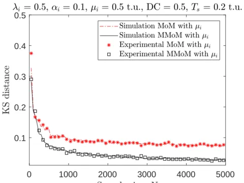
3.8 Simulation and Experimental Results . . . 52

3.9 Discussion of practical aspects . . . 57

3.10 Summary . . . 60

4 Estimation of Primary Activity Statistics under Imperfect Spectrum Sensing 63 4.1 Introduction . . . 63

4.2 System Model . . . 64

4.3 Methods Proposed to Overcome the Effect of Spectrum Sensing Errors on the Estimated Statistics . . . 65

4.3.1 Method 1 . . . 67

4.3.2 Method 2 . . . 68

4.3.3 Method 3 . . . 69

4.3.4 Other related Methods . . . 70

4.4 Simulation Results . . . 71

4.5 Configuration of the Proposed Methods . . . 76

4.6 Impact of the Primary User Activity Pattern . . . 78

4.7 Summary . . . 86

5 Cooperative Estimation of Primary Activity Statistics under Imperfect Spectrum Sensing 87 5.1 Introduction . . . 87

5.2 System Model and Problem Formulation . . . 88

5.3 Cooperative Estimation of the Distribution of Primary Channel Holding Times . . . 90

5.3.1 Direct Estimation Method (DEM) . . . 90

5.3.2 Method of Moments (MoM) . . . 90

5.3.2.1 Direct estimation of minimum . . . 90

5.3.2.2 Minimum based on MoM . . . 91

5.3.2.3 Minimum based on modified MoM . . . 91

5.4 Local State Reporting methods and Overhead . . . 91

5.4.1 Periodic Reporting Mechanism . . . 92

5.4.2 On/Off Reporting Mechanism . . . 92

5.4.3 Proposed Differential Reporting Mechanism . . . 93

5.4.4 Analysis of the Required Number of Reports . . . 94

5.5 Spectrum Sensing Data Falsification . . . 96 viii

5.6 Simulation and Experimental Methodology . . . 99 5.7 Simulation and Experimental Results . . . 100 5.8 Summary . . . 107

6 Conclusions and Future Work 113

6.1 Conclusions . . . 113 6.2 Future Work . . . 115

Bibliography 117

1.1 DSA/CR network architecture . . . 3 1.2 Dynamic spectrum access techniques. . . 5 1.3 Discrete-Time Markov chain model. . . 7 2.1 Considered model. Ts, T1,Tb₁ represent the sensing period, original busy

pe-riod duration and estimated busy pepe-riod duration, respectively. T_ex and Tey are the errors in period estimation. . . 16 2.2 The PDF of the error components: (a)fTx

e(t), (b) fTey(t). . . 18

2.3 The PDF of the combined error componentfTe(t). . . 18

2.4 Validation of the PDF of the estimated periods (λ1= 0.15, µ1 = 10t.u,E{T1}=

16.66 t.u.and Ψ = 0.5.) . . . 23 2.5 Validation of the CDF of the estimated periods (λ1 = 0.15, µ1= 10t.u,E{T1}=

16.66 t.u.and Ψ = 0.5.) . . . 24 2.6 KS distance for the observed and analytical model CDFs. . . 25 2.7 KS distance for the observed and analytical model CDFs. . . 25 2.8 Distribution estimation methods : (a) Direct estimation, (b) Method of

Mo-ments (MoM), (c) Modified Metod of MoMo-ments MMoM. . . 27 2.9 Block diagram of the PECAS prototype employed for hardware experiments

[103]. . . 30 2.10 PECAS hardware implementation [103]: (a) Transmitter, (b) Receiver. . . . 31 2.11 Relative error of the estimated minimum period _bµi. . . 32 2.12 Relative error of the calculated variance using (2.16) and (2.19). . . 33 2.13 The KS distance using direct estimation, MoM and MMoM. . . 34 2.14 KS distance for MoM and MMoM versus the sample size, both of the methods

assumed with perfectµ1 knowledge. . . 36

3.1 Required observation sample size for the estimation of the minimum period as a function of the sensing period (duty cycle Ψ = 0.5). . . 54 3.2 Maximum relative error of the estimated mean observed at the 95%

per-centile (ρ= 0.95) as a function of the sample size (duty cycle Ψ = 0.5). . . . 55 3.3 Maximum relative error of the estimated variance observed at the 95%

per-centile (ρ= 0.95) as a function of the sample size (duty cycle Ψ = 0.5). . . . 55 3.4 Maximum relative error of the estimated duty cycle at the 95% percentile

(ρ= 0.95) as a function of the sample size (duty cycle Ψ = 0.5). . . 56 3.5 KS distance of the estimated distribution at the 95% percentile (ρ = 0.95)

as a function of the sample size (duty cycle Ψ = 0.5). . . 56 3.6 Required sample size as a function of the desired estimation error for: (a)

mean, (b) variance, (c) channel duty cycle, and (d) distribution (µi = 0.1 t.u.,λi = 0.3 t.u.,αi = 0.05,Ts= 0.01 t.u., Ψ = 0.5,ρ= 0.95). . . 57 3.7 Estimated available data rate as a function of the estimated duty cycle. . . . 58

4.1 Estimation of period durations from spectrum sensing decisions: (a) under

perfect spectrum sensing, (b) under imperfect spectrum sensing [81]. . . 65

4.2 Sensing errors according to their location: (a) Original period, (b) Single de-tectable incorrect period, (c) Two dede-tectable incorrect periods, (d) Multiple detectable incorrect periods. . . 66

4.3 PMF of the number of consecutive sensing events affected by sensing errors (duty cycle (Ψ) = 0.8,µi = 10 time unit (t.u.),E{Ti}= 50 t.u.). . . 67

4.4 Estimated PU channel duty cycleΨ as a function of the number of periodsb used in the estimation (Ψ = 0.8,µi = 10 t.u., E{Ti}= 50 t.u.). . . 70

4.5 Performance of method 1. . . 73

4.6 Performance of method 2. . . 74

4.7 Performance of method 3. . . 77

4.8 Performance comparison of the methods considered in this chapter. . . 78

4.9 CDF of idle/busy periods (µi = 10 t.u.,E{Ti}= 50 t.u., Ψ = 0.5). . . 81

4.10 Estimation accuracy for the considered distributions under PSS. . . 82

4.11 Estimation accuracy with no reconstruction under ISS. . . 83

4.12 Estimation accuracy with method 4 under ISS. . . 84

4.13 Estimation accuracy with method 1 under ISS. . . 85

5.1 System model for cooperative primary traffic estimation with malicious users. 88 5.2 The operation for the considered reporting mechanisms. (a) The sensing stage at SU (it shows the required number of sensing events per SU. (b) Periodic reporting mechanism. (c) On/Off reporting mechanism (report for busy periods case). (d) Differential reporting mechanism. . . 93

5.3 Accuracy of the estimated distribution for different fusion rules and periodic reporting under sensing errors. . . 101

5.4 Different methods to estimate the distribution under periodic reporting: (a) Ts = 0.01 t.u., (b)Ts= 0.05 t.u., (c) Ts = 0.09 t.u. . . 102

5.5 Accuracy of the estimated distribution for different reporting mechanisms. . 103

5.6 Required number of reports under sensing errors (Pf a=Pmd= 0.1) for: (a) Periodic reporting, (b) On/Off reporting, (c) Differential reporting. . . 104

5.7 Reduction in the number of reports under PSS (Pf a=Pmd= 0). . . 105

5.8 Reduction in the number of reports under ISS (Pf a=Pmd= 0.1). . . 106

5.9 Accuracy of the estimated distribution for different fusion rules under both ISS (Pf a =Pmd= 0.01) and random attacks (MUs =K/4,Pa= 0.75). . . . 106

5.10 Accuracy of the estimated distribution under blind attacks: (a) MUs =K/2, (b) MUs = K/3, (c) MUs =K/4. . . 108 5.11 Accuracy of the estimated distribution under smart attacks: (a) MUs =K/2

and Pa= 0.25, (b) MUs = K/2 and Pa= 0.5, (c) MUs = K/2 andPa= 0.75.109 xii

= K/3 and Pa = 1 (Blind attack), (c) MUs = K/2 and Pa = 0.5 (Smart attack). . . 110

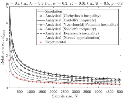
2.1 KS distance estimated using PECAS (experiment) versus simulation. . . 35 3.1 Relation between κ andρ for various concentration inequalities [108]. . . 46 4.1 Computational cost (complexity) analysis for the considered methods (Ψ =

0.8,µi= 10t.u.,Ts= 9.9 t.u.,Pf a=Pmd= 0.01). . . 76 4.2 Considered probability distribution models for PU idle/busy period durations. 80 4.3 Distribution parameters. . . 81

Symbol Description

CDF Cumulative Distribution Function

CR Cognitive Radio

CTMC Continuous-Time Markov Chain

CTSMC Continuous-Time Semi-Markov Chain

DC Duty Cycle

DEM Direct Estimation Method

Diff Differential

DSA Dynamic Spectrum Access

DTMC Discrete-Time Markov Chain

E Exponential Distribution

ECMA European Computer Manufacturers Association

ED Energy Detection

FC Fusion Centre

FCC Federal Communications Commission

G Gamma Distribution

GE Generalised Exponential Distribution

GP Generalised Pareto Distribution

GSM Global System for Mobile Communications

IEEE Institute of Electrical and Electronics Engineers

ISS Imperfect Spectrum Sensing

KS Kolmogorov-Smirnov

LTE Long-Term Evolution

LTM Longer Than the Minimum

MD Missed Detection

MMoM Modified Method of Moments

MoM Method of Moments

MU Malicious User

P Pareto Distribution

PDF Probability Distribution Function

PECAS Prototype for the Estimation of Channel Activity Statistics

PMF Probability Mass Function

PSS Perfect Spectrum Sensing

SDR Software Defined Radio

SINR Signal to Noise plus Interference Ratio

SNR Signal to Noise Ratio

SSDF Spectrum Sensing Data Falsification

STM Shorter Than the Minimum

SU Secondary User

W Weibull Distribution

WLAN Wireless Local Area Network

WRAN Wireless Regional Area Network

WS White Space

Introduction

Over the years, wireless technologies have evolved significantly to cope with increasingly challenging demands and trends ever since the first radio was invented by Nicola Tesla [1], blessed with the wide range of applications for wireless communications from wireless controlling devices to satellite systems and smart-phones. Wireless communications have had a huge impact on human lifestyle and having an internet access at any-time and any place has become essential. This popularity is followed by an exponential growth in the number of wireless connected devices. For instance, the expected number of connected devices per person by 2020 is 6.58 [2]. These devices could include smart-phones, TVs, computers and a wider range.

The growth in the number of users, applications, and the required bandwidth of mod-ern wireless communication systems has resulted in the Radio Frequency (RF) spectrum becoming increasingly crowded and plagued with interference. Hence, governmental agencies took control of RF management among transmitters [3].

Several field measurements of spectrum usage have demonstrated that the allocated spectrum is underutilized [4–8], with variations depending on access time (day/night) and geographical region (urban/rural), which means that the spectrum scarcity problem is a direct result from a fixed spectrum allocation. Therefore, new spectrum manage-ment paradigms are essential to efficiently access the radio resources. This situation motivated the introduction of more flexible spectrum allocation policies to overcome the shortcomings of the static allocation. As a result, the Dynamic Spectrum Access (DSA) paradigm based on the Cognitive Radio (CR) technology [9] has gained popularity to overcome the drawbacks and shortcomings of the currently inefficient static allocation schemes.

1.1

Dynamic Spectrum Access

The term Cognitive Radio was first proposed by Joseph Mitola [9]. In essence, a CR is a smart wireless device that is capable of tuning its communication parameters to adapt to the surrounding radio-environment. The DSA principle [10–12], relying on the CR paradigm, has been proposed to improve spectral efficiency [13]. In a CR network,

Secondary Users (SU) access the Primary User (PU) spectrum that is not being utilised (also known asspectrum holes) in an opportunistic manner to support spectrum reuse and increase spectrum efficiency [11, 14]. DSA/CR is a promising solution for the spectrum scarcity problem given the huge increase in the demand of wireless connected devices and sensors. It is expected from a CR to sense the primary channel in a periodic manner, to detect the presence of a PU. When a PU signal is detected, the SU has to stop operating at that frequency and has to search for a new empty frequency band. It is essential for a DSA/CR system to operate with minimal, non-harmful interference to the PU network even though PUs may use different modulations, transmission rates and powers, which adds more complexity to the operation of DSA/CR networks. DSA/CR networks are required to enable SUs to:

1. Determine the PU signal availability over the licensed spectrum. 2. Select the most appropriate channel for SU transmission.

3. Coordinate the access to available (idle) primary channels between SUs.

The access of CRs to TV white space is one of the examples of DSA systems [15], where the aim is to have CRs share the geographically unused TV bands in a non-interfering manner. Several standards for CR systems have been designed and deployed in TV white space including:

• The IEEE 802.22 Wireless regional area network (WRAN), which is the first cog-nitive radio standard [16, 17]. The IEEE 802.22 targets the use of UHF/VHF TV bands (54-862MHz) by SUs on a non-interfering basis, thus spectrum sensing is essential. In [18], different sensing methodologies for compatibility with 802.22 standard were investigated.

• While the IEEE 802.11 standard is well known for Wireless Local Area Network (WLAN) systems, the IEEE 802.11af standard aims to enable WLAN to operate in TV WS in an opportunistic manner [19].

• The IEEE 802.15.4m standard aims to enable ZigBee systems (low power and

complexity devices) to operate in television WS [20]. Some example applications include smart grid/utility, advanced sensor networks, and machine-to-machine net-works.

• The ECMA 392 standard aims to provide access to personal devices on television WS [21, 22]. Information on the TV channel occupancy can be obtained from databases accumulated by spectrum sensing to ensure interference-free coexistence with TV signal. The ECMA 392 standard fixes the available bandwidth to 6 MHz, 7 MHz, or 8 MHz, unlike IEEE 802.11af which provides flexibility on the SU available bandwidth.

Figure 1.1: DSA/CR network architecture [12].

Other examples include CRs access underutilised cellular network channels with higher channel capacity and lower intercell interference [23–26]. Benefiting from the ability to learn information on the primary network and adapt to it (by using previous channel knowledge to select the most appropriate channel with both higher SINR and WS) to create a cognition-inspired 5G cellular network [25]. Another example is cellular networks accessing the WS (unlicensed WiFi spectrum) dynamically in an opportunistic manner without causing interference or unfairness to WiFi networks as preserving fair coexistence is a main goal for DSA systems [27, 28].

1.2

Cognitive Network Architecture

The generic architecture of a DSA/CR network is shown in Fig. 1.1. Two main network components can be identified: the primary network and secondary network [12].

• Primary network. A primary network or a licensed network is an existing network infrastructure which has the right to access a specific spectrum band. For instance, cellular networks and TV broadcast are common examples of primary networks. A primary network consists of:

– Primary user. Primary or licensed is a user with a license to operate in a licensed band. The access to the channel is organised by the primary base station with a minimum interference by secondary users. For example, the

primary user is the TV receiver in the licensed TV band or the mobile phone in cellular networks.

– Primary base-station. Primary or licensed base station is the access point in the fixed infrastructure of the primary network. Primary base-station may have the capability to support both legacy and new protocols for network access by secondary users.

• Secondary network. A secondary or unlicensed network is a network with fixed infrastructure but without a license to operate in a spectrum band, thus accesses the spectrum in an opportunistic manner. A secondary network consists of:

– Secondary user. A secondary or unlicensed user is a network user without a license over the spectrum band. It can only access the spectrum in an opportunistic manner during spectrum holes (PU idle time or vacant areas).

– Secondary base-station. A secondary or unlicensed base station is part of the fixed infrastructure component which provides SUs with spectrum access capabilities without a spectrum license. As for cooperative spectrum sensing, the secondary base-station also serves as a fusion centre (FC) which gathers information from cooperative SUs to provide a global decision on spectrum availability.

– Spectrum broker. A spectrum broker or a scheduling server is a central net-work node that is in-charge of allocating spectrum resources to SUs (not necessarily from the same network).

1.3

Dynamic Spectrum Access Approaches

Hierarchical spectrum access allows the SU to access the primary spectrum under strict interference restrictions. There are three sub-categories of this scheme as illustrated in Fig. 1.2.

1. Interweave1. The SU is required to identify spectrum holes (when the PU channel is idle) and utilise this time and geographical location for transmission. As a result, the interference on the PU network would not exist since PU and SU transmissions are orthogonal. Such sharing model is not required to follow any constraints on transmission power. However, SUs are required to periodically monitor the PU channel to determine the activity status (i.e., busy or idle) and vacate the channel when PU is active [29].

2. Underlay. The SU accesses the PU channel at any time but with low transmission power to reduce harmful interference on PU [30–32]. Such sharing model can be utilised for short range communication devices. In this model, the tolerable

Time Time Time Power Power Power PU signal SU signal Interweave Underlay Overlay

Portion of SU power used to improve PU signal

Figure 1.2: Dynamic spectrum access techniques.

interference level at PU is defined by the interference temperature which is specified by the Federal Communications Commission (FCC) [33].

3. Overlay. The SU also accesses the PU channel at any time but some of the SU power is utilised to assist the transmission of PU and compensate for the interference generated by the remaining power allocated to the SU transmission [34].

This work focuses on the interweave approach.

1.4

Spectrum Sensing

Spectrum sensing is a key enabling technology for CR operation in interweave mode, as it allows SUs to detect the presence/absence of PU traffic, which is essential to reduce the interference [14, 35–39]. Spectrum sensing can also be utilised to capture PU traffic activity for the analysis stage of spectrum characterization. Spectrum sensing can be sub-characterised to two different techniques: non-cooperative and cooperative based sensing.

1.4.1 Non-Cooperative Sensing

The main hypothesis here is the presence of the PU signal. Usually, the received signal at the SU is composed of PU’s signal plus noise when the PU is active. Otherwise, the SU receives only noise when the PU is idle. There are three main methods for PU detection.

• Energy detection. Energy detection (ED) provides an optimal solution for detection when no information on the signal is available [40]. However, the performance of ED is highly dependent on the received signal energy and noise level [41, 42]. The received signal energy is compared with a predefined threshold and a decision is made stating that PU is active if the signal energy is higher than the threshold. Otherwise, the PU is assumed to be idle. The ED proved to be the most practical one, as most of the time spectrum sensing is performed using low cost devices in practice and this method works regardless of the PU signal format.

• Matched filter detection. Matched filter approach provides an optimal solution for additive noise type as it maximises the SNR, however it requires a prior knowledge of the PU signal, for example the modulation type, the pulse shape, and the packet format [12]. Matched filter techniques proved to deliver a good detection performance under low SNR environment [43, 44].

• Feature detection. Feature detection targets exploiting the partial knowledge of PU signal. For instance cyclostationary feature detection utilises the periodicity in modulated signals (periodic for modulated signals and aperiodic for noise) [45, 46]. The autocorrelation based detection assumes a wide-sense stationary PU signal and exploits the autocorrelation feature to identify PU signal [47].

1.4.2 Cooperative Sensing

Single based sensing faces reliability problems during the detection of weak signals (due to fading/shadowing) at levels well below the noise floor [48, 49]. Cooperative sensing exploits the spatial diversity of SUs to enhance spectrum sensing [50–52]. In general, cooperative sensing can be classified into distributed cooperative sensing and centralized cooperative sensing. In the distributed cooperative sensing, the SUs exchange their local sensed PU states [53]. While in the centralized cooperative sensing, the SUs report their local sensed PU states to a central server known as the fusion centre (FC) for a global decision based on a specific fusion rule [54].

1.5

Spectrum Availability Modelling

An SU access the licensed user spectrum during idle time in an opportunistic and non-interfering manner. Hence, the performance of an SU is highly dependent on PU activity. Several approaches have been proposed in the literature to model PU activity pattern [11, 55]. In this section, time-dimension models based on Markov chain approach are discussed as it is the most popular modelling method for PU activity pattern.

1.5.1 Two State Markov Chain

At any given time instant, the primary channel may be either busy or idle (binary state). The binary state space for PU channel may be denoted by S ={s0, s1}, where the s0

S

S

p01

p10

p11 p00

Figure 1.3: Discrete-Time Markov chain model.

indicates an idle channel and thes1 indicates a busy channel. At any given timet, the

channel state can be either S(t) = {s0} or S(t) = {s1}. The two state Markov chain

process can be modelled as either discrete-time or continuous-time based on the time indext. The discussion on both these models are provided below.

1.5.1.1 Discrete-Time Markov Chain

In a Discrete-Time Markov chain (DTMC), the PU channel state changes at discrete time intervals (i.e., t = tx = xTc, where x is a non-negative integer representing the step number and Tc the time duration between two consecutive state changes [56]. The probability of state transition is defined as pij. Hence, if the current state is i, the probability of state changejis defined aspij [57]. The transition matrix of probabilities can be expressed as:

P = " p00 p01 p10 p11 # = " 1−Ψ Ψ 1−Ψ Ψ # , (1.1)

where Ψ is the duty cycle of the PU. pij represents the probability of system transition between idleS0 and busyS1 states.

1.5.1.2 Continuous-Time Markov Chain

In the Continuous-Time Markov Chain (CTMC), the time index takes any continuous value. The channel remains in one state for a random time before shifting the state. The next transition is independent of the state history. The channel holding times (activity time) are modelled as an exponentially distributed random variable. In the literature, CTMC is one of the most commonly deployed models for DSA/CR [58–62].

Field measurements for real wireless communications have shown that the exponen-tial distribution is not the most accurate model for PU holding times. Instead, the Continuous-Time Semi-Markov Chain (CTSMC) model is used to model the occupancy activity [63–65]. In CTSMC, the PU holding times can follow any arbitrary distribution [11].

Other differences between the CTMC/CTSMC and DTMC models is in CTM-C/CTSMC it is possible to control the mean, variance and minimum transmission dura-tion of the produced occupancy periods, while this is not possible for DTMC as only the

duty cycle is controllable. In this thesis, both the CTMC and CTSMC are considered to model PU activity time.

1.6

Estimation of Primary Statistics

The estimation of PU traffic statistics (duration of the idle/busy periods of a channel) is inferred from the spectrum sensing decisions. SUs sense the channel with a finite sensing periodTs(shorter than the minimum period duration). At every sensing event, a binary decision is made,H0 for idle and H1 for busy. When a change in the observed

state occurs, the time interval elapsed since the last is computed to make the estimation of the original real period. The process is repeated for a sufficiently large number of periods until enough data is available. The set of observed periods is then used by the CR to estimate the activity statistics of the PU channel. Some examples of relevant statistics commonly used in the DSA/CR literature are the minimum period duration, the moments (mainly, the mean and the variance), the channel duty cycle and the underlying distribution. The estimation of these statistics will be investigated in this thesis.

Unfortunately, spectrum sensing suffers from practical impairments. The impair-ments include: i) the estimation of primary statistics based on a finite sensing period, which determines the resolution of estimation for each individual period and imposes a fundamental limit on the accuracy of estimation of individual periods and the corre-sponding statistics; ii) the finite number of observed periods given that the time required to observe the channel to obtain accurate estimation of the statistics is limited; iii) the presence of sensing errors in the estimation process. The individual estimated period durations will be affected significantly by these practical impairments, which could lead to either under/over estimation of statistics. The impact of all these degrading effects will be investigated in this thesis.

1.7

Motivation and Objectives

The knowledge of the primary activity statistics such as the minimum, mean and variance of the on/off period durations, the channel duty cycle, and the underlying distribution can be employed to access the spectrum more effectively and improve the CR system performance [66–68]. This can be achieved by selecting the most appropriate channel for transmission [69], reducing the switching time delay [70, 71], adapting the parameters of CRs’ medium access control (MAC) layer [72], selecting an appropriate threshold in case of using energy detection [73], forecasting the primary occupancy pattern to minimise the interference [74–76], or fight against attacks [77] for the case of cooperative spectrum sensing and thus increase the overall spectrum efficiency.

An example on the benefits of having knowledge of the primary distribution is when a packet needs to be transmitted. The packet size is used to estimate the approximated

time that its transmission would require based on known operation parameters (e.g., channel bandwidth, modulation and coding schemes and so on). Once the estimated transmission time required for the packet is known, the DSA/CR system selects the primary channel with the highest probability to provide a continuous idle/off period that is at least as long as the time required for the packet transmission. Such probability can be obtained from the distribution of idle/off times.

This information could be obtained from spectrum sensing or other alternatives such as databases. However, the sensing-based approach has significant advantages including lower cost and complexity, independence of external systems and better suitability for highly dynamic radio environments [78]. In this thesis, the problem of estimating the PU traffic statistics based on spectrum sensing is investigated.

In the literature, several studies have considered the problem of estimating primary activity statistics based on sensing decisions, mostly focusing on the estimation of the channel duty cycle. In [79], the estimation of the channel occupancy rate (duty cycle) based on different approaches was studied analytically in the presence of sensing errors. A mathematical analysis on the estimation of the mean on/off durations, as well as the duty cycle under DSA, was presented in [80]. In [10] several methods for the classifi-cation of such distribution were proposed under the assumption of no sensing errors. To overcome the degrading effect of sensing errors on the estimated primary activity statistics, several algorithms were proposed in [81]. Nevertheless, several questions re-main without sufficient answers such as closed form expressions for the estimation of the distribution of busy/idle periods based on spectrum sensing, how big the sample size of busy/idle periods should be to have an accurate estimation of the statistics, and new methods to improve the estimation of the statics under sensing errors.

In this context, this thesis aims at filling the existing gaps by providing answers to these questions. The objective in this line is to provide closed-form expressions that characterise the accuracy of the estimated statistics as function of the practical impairments such as the use of finite sensing period and/or sample size (for the PSS case) and develop new methods to accurately estimate the PU traffic statistics in the presence of sensing errors (for the ISS case).

Moreover, the potential benefits arising from cooperative estimation of the PU statis-tics is investigated as well, as a means to improve the detection performance taking advantage of the spatial diversity for multiple cooperating nodes [82, 83], it is utilised here to provide an accurate estimation of the primary traffic under imperfect spectrum sensing (ISS). Unfortunately, the improvement in performance achieved by cooperation is hindered by the increase of cooperation overhead. Several studies have aimed at im-proving energy efficiency in cooperative spectrum sensing by reducing the consumed power at each step of the cooperative sensing operation [84]. For instance, reducing the power consumed during the sensing stage [85, 86], or at the reporting stage [87–89] by selecting the most useful SUs for local states reporting to the fusion centre (FC). Another problem that has not attracted enough attention is the estimation of primary

traffic statistics under spectrum sensing data falsification (SSDF) attacks. CR systems are more susceptible to SSDF attacks (also known as Byzantine attacks) and to the presence of greedy users who send false reports to gain more access to primary channels. Multiple studies have considered the effect of attacks on the sensing process [90–92], however their main aim is the estimation of the probability of primary signal detection instead of the PU traffic statistics. In this thesis, another objective is to investigate the effect of these attacks on the estimation of primary traffic statistics and develop a new reporting mechanism with the aim of reducing the number of required transmissions at each reporting stage while guaranteeing a secure sensing reporting and therefore an accurate estimation of the PU traffic statistics.

1.8

Thesis Contributions

This thesis aims to address the fundamental problem of accurately estimating the pri-mary traffic statistics under different scenarios. The main contributions can be sum-marised as follows:

1. An analytical model is developed to link the spectrum sensing period with the observed PU traffic statistics and quantify the effects of the spectrum sensing period on the resulting estimation accuracy.

2. A novel approach based on a modified version of the Method of Moments (MoM) is proposed to remove the impact of using a finite sensing period on the estimated PU distribution and improve its accuracy.

3. An analytical model is developed to link the sample size with the observed PU traffic statistics and quantify the effects of the observed sample size on the resulting estimation accuracy.

4. Three novel algorithms are proposed to enhance the estimation of primary activity statics under imperfect spectrum sensing given the knowledge of the minimum transmission duration. Moreover, the impact of different primary distributions on the performance is investigated as well.

5. A detailed study on the cooperative estimation of the PU activity statistics (in particular, the distribution of the channel holding times) under both spectrum sensing errors and SSDF attacks is carried out, which shows improvements in the estimation accuracy. A novel algorithm to reduce both the signalling overhead and estimation errors under SSDF attacks in the cooperative scenario is proposed and compared to other algorithms from the literature showing performance improve-ments.

1.9

Thesis Outline

The remainder of this thesis is organised as follows.

Chapter 2, investigates the impact of the sensing period on the accuracy of the estimated primary actively statistics. Closed-form expressions for the PDF and CDF of the periods observed at the SU as a function of the original distribution at the PU and the sensing period employed by the SU are derived. Then, closed form expressions for the maximum observed error as a function of the sensing period and distribution parameters are provided as well. New methods to improve the estimation of the distribution are proposed. Finally, the simulation and experimental results of the proposed methods are analysed thoroughly.

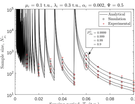
The problem of sample size effect on the distribution estimation accuracy is dis-cussed in Chapter 3. First, a detailed mathematical analysis on the sample size required to provide an arbitrarily accurate estimation of the minimum period, the mean and variance of the observed periods, the channel duty cycle and the underlying distribu-tion of the observed periods is provided. The obtained analytical results depend on the real/actual parameters of the PU traffic, which are unknown to the SU; this problem is overcome with an iterative stopping algorithm that enables an accurate estimation of the required sample size in practical implementations. Finally, the simulation and experimental methodology employed to validate the correctness and accuracy of the analytical results is described along with the obtained results.

In Chapter 4, the formal description of the problem of estimating the PU activ-ity statistics under imperfect spectrum sensing is first provided. The novel proposed algorithms to mitigate the impact of sensing errors are explained in detail along with other previous methods proposed in the literature. The performance of the proposed algorithms (obtained by simulation) are analysed and compared with other algorithms along with the discussion on the configuration of spectrum sensing based on the obtained results. Then, different statistical distributions to model the PU activity are introduced and the performance of the proposed algorithms is assessed through simulations under the different considered PU traffic models.

In Chapter 5, the cooperative estimation of primary traffic statistics is considered. First, the structure of the cooperative system is considered along with the cooperative estimation of primary signal durations and cooperative algorithms utilised. Different estimation methods for the cooperative estimation of the primary governing distribution are described. The problem of increasing overhead along with an efficient reporting mechanism are described as well and the problem of SSDF attacks and how to protect against them are also discussed. The performance of the proposed methods is analysed thoroughly by means of simulation and hardware experiments.

Finally, Chapter 6 highlights the main findings and conclusions of this thesis and suggests some ideas for extension in future work.

1.10

List of Publications

Relevant Journal Publications

1. A. Al-Tahmeesschi, M. L´opez-Ben´ıtez, D. Patel, J. Lehtom¨aki and K. Ume-bayashi, “On the Sample Size for the Estimation of Primary Activity Statistics Based on Spectrum Sensing,” IEEE Transactions on Cognitive Communications and Networking. (Accepted)

2. A. Al-Tahmeesschi, M. L´opez-Ben´ıtez, V. Selis, D. Patel, J. Lehtom¨aki and K. Umebayashi, “Cooperative Estimation of Primary Traffic Under Imperfect Spec-trum Sensing and Byzantine Attacks,” IEEE Access. (Accepted)

3. M. L´opez-Ben´ıtez, A. Al-Tahmeesschi, D. Patel, J. Lehtom¨aki and K. Ume-bayashi, “Estimation of Primary Channel Activity Statistics in Cognitive Radio Based on Periodic Spectrum Sensing Observations,” IEEE Transactions on Wire-less Communications. (Under revision)

Relevant Conference Publications

1. A. Al-Tahmeesschi, M. L´opez-Ben´ıtez, J. Lehtom¨aki and K. Umebayashi, “In-vestigating the Estimation of Primary Occupancy Patterns under Imperfect Spec-trum Sensing,” 2017 IEEE Wireless Communications and Networking Conference Workshops (WCNCW), San Francisco, CA, 2017, pp. 1-6

2. A. Al-Tahmeesschi, M. L´opez-Ben´ıtez, K. Umebayashi and J. Lehtom¨aki, “Ana-lytical study on the estimation of primary activity distribution based on spectrum sensing,” 2017 IEEE 28th Annual International Symposium on Personal, Indoor, and Mobile Radio Communications (PIMRC), Montreal, QC, 2017, pp. 1-5. 3. A. Al-Tahmeesschi, M. L´opez-Ben´ıtez, J. Lehtom¨aki and K. Umebayashi,

“Ac-curate estimation of primary user traffic based on periodic spectrum sensing,” 2018 IEEE Wireless Communications and Networking Conference (WCNC), Barcelona, 2018, pp. 1-6.

4. A. Al-Tahmeesschi, M. L´opez-Ben´ıtez, J. Lehtom¨aki and K. Umebayashi, “Im-proving primary statistics prediction under imperfect spectrum sensing,” 2018 IEEE Wireless Communications and Networking Conference (WCNC), Barcelona, 2018, pp. 1-6.

5. M. L´opez-Ben´ıtez,A. Al-Tahmeesschi, K. Umebayashi and J. Lehtom¨aki, “PECAS: A Low-Cost Prototype for the Estimation of Channel Activity Statistics in Cog-nitive Radio,” 2017 IEEE Wireless Communications and Networking Conference (WCNC), San Francisco, CA, 2017, pp. 1-6.

6. M. L´opez-Ben´ıtez, A. Al-Tahmeesschi and D. Patel, “Accurate Estimation of the Minimum Primary Channel Activity Time in Cognitive Radio Based on Pe-riodic Spectrum Sensing Observations,” European Wireless 2018; 24th European Wireless Conference, Catania, Italy, 2018, pp. 1-6.

Other Publications

1. Z. Wei, X. Zhu, S. Sun, Y. Huang, A. Al-Tahmeesschi and Y. Jiang, “Energy-Efficiency of Millimeter-Wave Full-Duplex Relaying Systems: Challenges and So-lutions,” in IEEE Access, vol. 4, pp. 4848-4860, 2016.

2. Z. Wei, X. Zhu, S. Sun, Y. Jiang,A. Al-Tahmeesschiand M. Yue, “Research Is-sues, Challenges, and Opportunities of Wireless Power Transfer-Aided Full-Duplex Relay Systems,” in IEEE Access, vol. 6, pp. 8870-8881, 2018.

Impact of the Sensing Period

under Perfect Spectrum Sensing

2.1

Introduction

DSA/CR users can utilize spectrum sensing decisions to obtain information on PU chan-nel activity. The PU chanchan-nel is sensed periodically by DSA/CR users to decide the channel state (busy or idle) at every sensing event based on a signal detection algorithm [36]. These spectrum decisions can be used to estimate the durations of the idle and busy periods. Unfortunately, the estimation of PU activity periods and statistics by means of spectrum sensing (periodic channel observations) suffers from practical limitations, such as finite sensing duration and limited observation time. These limitations reduce the accuracy of PU parameters estimated by DSA/CR users as discussed in Section 1.6. The main interest and focus of this chapter is to first analyse the impact of the spec-trum sensing period on the accuracy of the estimated PU activity statistics in particular, the distribution of PU busy/idle periods. A complete characterisation of the PU activity statistics is provided. Despite being an elemental problem of crucial importance for CR systems, this has never been considered or analysed before in the existing literature. Second, to improve the estimation of PU activity statistics (focusing on the distribution of PU busy/idle periods), a novel approach is proposed based on the Method of Moments (MoM) to improve the PU distribution estimation under finite spectrum sensing. The impact of sensing errors (i.e., false alarms and missed detections) is out of the scope of this chapter and hence a high signal-to-noise ratio (SNR) scenario with no sensing errors is considered. The imperfect sensing scenario will be addressed in Chapters 4 and 5.

The contributions of this chapter can be summarised as follow:

1. Analytical expressions are derived for both the Probability Density Function (PDF) and the Cumulative Distribution Function (CDF) observed at the SU taking into account the effect of the spectrum sensing period.

2. Analytical expressions are derived for the maximum error in the distribution taking into account the effect of the spectrum sensing period.

Idle

Idle

𝑇

𝑇

𝑇

𝑇

𝑇

𝑇

𝑇

𝑇

𝑇

…

…

Busy

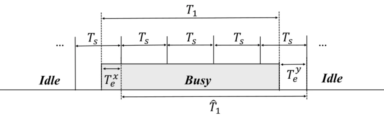
Figure 2.1: Considered model. Ts, T1,Tb1 represent the sensing period, original busy

period duration and estimated busy period duration, respectively. Tx

e andTey are the

errors in period estimation.

3. The effect of the spectrum sensing period on the distribution observed at the SU is studied.

4. A novel method to palliate the effects of spectrum sensing on the distribution estimation is proposed. Experimental results are provided to validate the proposed method and simulations.

2.2

System Model

A single SU is considered to detect PU activity. The SU performs spectrum sensing decisions with periodicity Ts time units (t.u.) to detect the presence/absence of PU signal on a specific frequency band. The results of the decisions are introduced as a binary alternating state: busy when the PU signal is present at the SU and idle when the PU signal is absent at the SU. The computed elapsed time (at SU) between two PU state changes is considered as an estimationTb_i of the real period duration T_i (i= 0 for

idle periods andi= 1 for busy periods) as illustrated in Fig. 2.1, where the estimation of the duration of a busy period is shown (idle periods can be estimated using the same method). The estimated period durations are integer multiples of Ts (i.e., Tb_i = kT_s,

with k ∈ N+, where k represents the number of sensing events within the estimated period. A similar model was considered in [81].

As discussed in Section 2.1, a high SNR scenario is assumed with no sensing errors so that the only degrading effect considered in this study is the impact of the finite sensing period Ts, which is the aspect of interest in this chapter. The PU activity periods Ti can be sensed accurately in case the channel is sensed exactly at the points of PU state change. In practice the SU is de-synchronised with the PU channel activity and the PU channel is sensed at arbitrary time instants every Ts time units (t.u.). As a result,

the estimated periods Tb_i depend not only on the original periods T_i but also on the

employed sensing period Ts. The first main objective of this chapter is to explore the relation between the original periodsTi and the estimated periodsTb_i as a function of the

sensing periodTs. To this end, closed-form expressions are developed for the PDF/CDF of Tb_i as a function of the PDF/CDF ofT_i and T_s.

2.3

Distribution of the Estimated Periods

2.3.1 Calculation of the Estimated distribution

The estimated periods Tb_i can be expressed as a function of the original periods T_i as b

Ti=Ti+Te, whereTeis the error component, which according to the model of Fig. 2.1 is given byTe=Tey−Tex. As it can be appreciated from Fig. 2.1, bothTexandT

y

e can take any value between 0 and Ts. Reasonable and intuitive assumptions that both of them are independent and follow a uniform distribution (i.e., T_ex and Tey ∼ U(0, Ts)). Both assumptions can be verified from Fig. 2.2, which was obtained by simulating the sensing of a sufficiently high number of exponentially distributed periods Ti using a sensing period Ts = 5 t.u., recording the error components Tex and T

y

e, and computing their normalized histograms (i.e., PDFs). As it can be observed, the assumptions of uniform distribution and independences for the T_ex and Tey error components are correct. In some specific cases, this assumption might not be completely accurate, depending on the particular value of the involved parameters. The effect, however, was observed to be minimal, with just a small ripple in the shape of the PDF of Te which is negligible. Moreover, the assumption of independency betweenT_ex andTey is necessary to make the problem under study analytically tractable.

The PDF for the triangular distribution of Te is:

fTe(t) =                0 t < −Ts Ts+t T2 s −Ts≤t≤0 Ts−t T2 s 0≤t≤Ts 0 t > Ts. (2.1)

This model can be verified from simulation results as shown in Fig. 2.3.

The PU state holding times (T0 and T1) are random variables assumed to be

inde-pendent and exponentially distributed [71]. The exponential distribution is the most common model used to describe the periods of the on/off states in the literature [80, 93] even though it is proven not to be the most accurate since other distributions provide better fit for real scenarios such as the generalized Pareto, Gamma or even more compli-cated distributions [64]. The exponential distribution is utilised because of its analytical traceability. The PDF and CDF for the exponential distribution are given as [94]:

(a) (b)

Figure 2.2: The PDF of the error components: (a)fTx

e(t), (b)fTey(t).

Figure 2.3: The PDF of the combined error componentfTe(t).

fTi(t) =    0 t < µi λie−λi(t−µi) t≥µi, (2.2) FTi(t) =    0 t < µi 1−e−λi(t−µi) _t≥µ i, (2.3)

whereλiis the distribution scale parameter andµiis the distribution location parameter (also the smallest value for the PU activity period).

f b Ti(t) =fTi(t)∗fTe(t) = Z ∞ −∞ fTi(τ)·fTe(t−τ)dτ, (2.4)

where fTi(t) and fTe(t) are given by (2.2) and (2.1) respectively. The operator ∗ refers

to the convolution operation. The resulting expression for the PDF f

b

Ti(t) is shown in

(2.5) while the CDF F

b

Ti(t) can be obtained through the direct integration of fTbi(t) as

shown below: F b Ti(t) = Z t −∞ f b Ti(τ)dτ. (2.6)

The final CDF expression can be seen in (2.7).

Note that the distributions in (2.5) and (2.7) have a continuous domain, while the actual distributions of the periods observed at a SU are discrete since the periods esti-mated from spectrum sensing as shown in Fig. 2.1 are integer multiples of the employed sensing period (i.e.,Tb_i =kT_s, k= 1,2,3. . .). Such discrete distribution can be obtained

by evaluating (2.5) and (2.7) at the right points of each interval/bin of the PDF and CDF, respectively, as: g b Ti(k) =fTbi(kTs), (2.8) G_Tb i(k) =FTb_i((k+ 1/2)Ts). (2.9)

The set of obtained expressions provide closed-form relations between the distribu-tions of the original periodsTi resulting from the PU transmission (and its parameters

µi, λi), the distribution of the estimated periods Tb_i as observed by the SU based on

spectrum sensing decisions, and the employed sensing period Ts. These mathematical results are useful to evaluate the impact of the employed sensing period on the accuracy of the distributions estimated by the SU and can find many practical applications such as mathematical analysis, simulation or system design (e.g., determine the maximum value of Ts required for a given level of estimation accuracy).

2.3.2 Error of the Estimated Distribution

To better understand the sensing period effect on the observed distribution, we utilize the well-known Kolmogorov-Smirnov (KS) distance. This is the most commonly used metric to quantify the error between two distributions. The KS distance is defined as the largest absolute error between two continuous CDFs and given as follows [96]:

DKS = sup t FTi(t)−FTbi(t) . (2.10)

To find the value of t that maximises the distance (DKS), the partial derivative of the absolute difference in the KS distance is taken and equated to zero as follows:

∂[FTi(t)−FTbi(t)]

f b T i ₍ t ) =                    0 t < µ i₋ T s T s + t − µ i T 2 s − 1 λ i_T 2 s 1 − 1 λ i _f T i₍ t + T s₎ µ i − T s ≤ t < µ i T s − t + µ i T 2 s + 1 λ i_T 2 s 1 + 1 λ i _f T i₍ t + T s₎ − 2 λ i _f T i₍ t ) µ i ≤ t ≤ µ i + T s 1 ( λ i_T s₎ 2 f T i₍ t + T s₎ − 2 f T i₍ t ) + f T i₍ t − T s₎ t > µ i + T s (2.5) F b T i ₍ t ) =                          0 t < µ i − T s t ₂ − ( µ i − T s₎ 2 2 T 2 s − h 1 − λ i₍ T s − µ i₎ i ( t + T s − µ i₎ λ i_T 2 s + 1 ( λ i_T s₎ 2 F T i₍ t + T s₎ µ i₋ T s ≤ t < µ i µ 2 i − t ₂ 2 T 2 s − 2 − λ i_T s 2 λ i_T s + h 1 + λ i₍ T s + µ i₎ i ( t − µ i₎ λ i_T 2 s + 1 ( λ i_T s₎ 2 F T i₍ t + T s₎ − 2 F T i₍ t ) µ i ≤ t ≤ µ i + T s 1 + 1 ( λ i_T s₎ 2 F T i₍ t + T s₎ − 2 F T i₍ t ) + F T i₍ t − T s₎ t > µ i + T s (2.7)

The largest difference occurs at t= µi which is found through numerical methods. Since FTi(µi) is zero at t=µi, the final expression for the KS distance will be:

DKS =F_Tb i(µi) = 1 2− 1 λiTs +1−e −λiTs (λiTs)2 . (2.12)

Expression (2.12) provides an easy and accurate tool to mathematically calculate the KS distance between the estimated and original CDFs as a function of the employed sensing period. Moreover, expression (2.12) can be used to calculate theTsrequired for a given target estimation error.

2.3.3 Numerical Results

In this section, first the accuracy of the proposed model for both PDF and CDF will be assessed, then the effect of the sensing period on the distribution estimation. For all the considered cases the sensing period is lower than the minimum PU activity time (Ts< µi). This is required to ensure that no activity periods are missed in the sensing process (the shortest detectable period isTs), which would otherwise lead to significant estimation errors. Notice that this consideration implicitly assumes that the minimum PU activity timeµi is known to the SU so that the value ofTscan be configured not to exceed µi. This assumption is realistic since the value of µi is available for some well-known standardised radio technologies (e.g., the time-slot duration of GSM or LTE) or can be obtained with other methods such as blind recognition/estimation [97] or from PU beacon signals [98].

The simulation results are obtained by following steps listed below:

1. Generate idle/busy periods’ lengths Ti following a generalized exponential distri-bution.

2. Perform idle/busy sensing decisions H0/H1 on the generated sequence in step 1

everyTs time units (t.u.).

3. Calculate the idle/busy lengths Tb_i using H₀/H₁ sequence from step 2 estimated

under PSS.

4. Compute the CDF/PDF of the idle/busy lengths obtained in step 3, and compare with the CDF/PDF of the original lengths in step 1.

On the other hand, analytical results are obtained by applying the system parameters into the derived expressions. For example, 2.12 is used find the error in the CDF (KS distance).

Fig. 2.4 shows the busy periods PDFsf_Tb

i(t) obtained from simulation and analytical

= 1, 3 and 5 t.u.). The discrete expressiong

b

Ti(k) has not been included for clarity but

its corresponding values can be easily obtained as the values of the analytical expression

f

b

Ti(t) atkTs. It can be appreciated that the closed form analysis provides an excellent

fit with the simulation results for all the considered scenarios, which verifies the validity of the mathematical expression obtained for the PDF. Moreover, Fig. 2.4 shows the effect of sensing period Ts on the discrete estimated PDF gTbi(k). High sensing periods

give higher estimation errors and vice versa.

Fig. 2.5 shows the busy periods CDFs obtained from simulation G

b

Ti(t) (discrete)

and analytical expressionF

b

Ti(t) versus the original distributionFTi(t) for multiple values

of sensing periods (Ts = 1, 3 and 5 t.u.). The closed form analysis provides an excellent fit with the simulation results for all the considered scenarios, which verifies the validity of the mathematical expression obtained for the CDF. The stair shape of the observed CDF G_Tb

i(t) represents the effect of the spectrum sensing operation and the resulting

discrete observed periods.

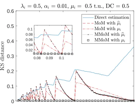
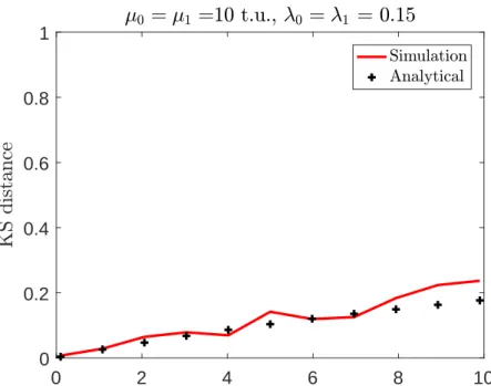
Fig. 2.6 shows the KS distance for the simulated and analytical CDF with respect to the original distribution. The x-axis represents the duration of sensing period in time units and the y-axis represents the KS distance. Since the sensed CDF is a discrete distributionG

b

Ti(t), it is to be transformed to a continuous form for comparison purposes.

To this end, the CDF frequency polygons are utilised [99], where the mid points of the discrete CDF are joined together and extended to include the zero frequency cases from left of the normalised histogram and hence obtain the continuous form of the CDF. As it can be appreciated from Fig. 2.6, the analytical expression (2.12) gives an excellent prediction of the estimation error. High Ts values will result in larger errors in the estimation of the PU activity pattern, however the resulting estimation error can be reduced by decreasing Ts.

Fig. 2.7 analyses the impact of different λi values (λi = 0.15,0.25,0.35 and 0.45) on the KS distance based on (2.12). Fig. 2.7 implies that not only the value of Ts has an impact on the estimated error (KS distance) but also the value ofλi (distribution scale). The KS distance increases with higher values of λi. The analytical result in (2.12) can be used as shown in Fig. 2.7 to determine the maximum value ofTs required for a given level of estimation accuracy of the distribution.

2.4

Methods for Accurate Estimation of the Distribution

This section proposes new methods to overcome the impact of a finite sensing period on the estimated distribution. To this end, it is first necessary to analyse how the sensing period affects the estimation of the minimum period, as well as the mean and variance of the estimated periods.

Figure 2.4: Validation of the PDF of the estimated periods (λ1 = 0.15, µ1 =

0 10 20 30 40 50 0 0.2 0.4 0.6 0.8 1 0 10 20 30 40 50 0 0.2 0.4 0.6 0.8 1 0 10 20 30 40 50 0 0.2 0.4 0.6 0.8 1

Figure 2.5: Validation of the CDF of the estimated periods (λ1 = 0.15, µ1 =

0 2 4 6 8 10 0 0.2 0.4 0.6 0.8 1

Figure 2.6: KS distance for the observed and analytical model CDFs.

0 2 4 6 8 10 0 0.2 0.4 0.6 0.8 1

2.4.1 Estimation of the Minimum Period Duration

As mentioned earlier, CR systems estimate the PU activity pattern based on the discrete observation periodsbτi ={Tbi,n}

N

n=1, whereN represents the number of observed periods

(sample size of_bτi). In order to have accurate estimations of the distribution, the sample size N has to be sufficiently large. The minimum activity duration was simulated in [81], nevertheless a closed form expression for the estimation of minimum PU activity time (µ_bi) is provided with a link to the sensing period (Ts). It can be shown that the estimated periods can also be expressed as:

b Ti = Ti Ts +ξ Ts, (2.13)

where b·cdenotes the floor operator and ξ ∈ {0,1} is a Bernoulli random variable [57], introduced to reflect the fact that the same original period Ti can lead to two possible estimated periods, eitherTb_i=kT_sorTb_i= (k+ 1)Ts, depending on the relative (random)

position of the sensing events with respect to the beginning/end ofTi. Hence, µbi can be

expressed as:

b

µi= min(τbi)≈min(Tbi) = min

Ti Ts +ξ Ts = µi Ts Ts, (2.14)

note that the minimum value in (2.14) corresponds to min(Ti) =µi and min(ξ) = 0.

2.4.2 Estimation of the Mean and Variance of Period Durations

Given a set of N (discrete) estimated periods τ_bi = {Tb_i,n}N_n=1, the mean E(Tb_i) and

variance V(Tbi) of the provided durations can be estimated based on the corresponding

sample moments: E(Tbi) = 1 N N X n=1 b Ti,n, (2.15) V(Tbi) = 1 N−1 N X n=1 (Tb_i,n−_E(Tbi))2. (2.16)

The impact of Ts on the estimated moments (first and second) can be determined as follows:

E(Tb_i) =E(T_i) +E(T_e) =E(T_i), (2.17) V(Tbi) =V(Ti) +V(Te) =V(Ti) +

T_s2

6 , (2.18)

where Ti and Te are assumed to be mutually independent, and E(Tb_e) and V(Tb_e) have

been replaced with the mean and variance of the triangular distribution in (2.1). The triangular distribution in this case has a mean value of zero (i.e., E(Te) = 0), which means that the duration of Ts does not affect the calculation of the mean value. On

the other hand, the calculation of the variance is affected by a factor ofT_s2/6. Based on (2.18), the effect ofTscan be minimized by applying to (2.16) the appropriate correction factor:

V(Tei) =V(Tbi)−

T_s2

6 , (2.19)

where V(Te_i) is the observed variance after correction. This approach eliminates the

impairments imposed by the sensing operation with duration of Ts in the estimated moments and is able to provide an accurate estimation of the real moments ofTi, based on the estimated period durationsτ_bi, as long as the sample sizeN is sufficiently large.

Spectrum

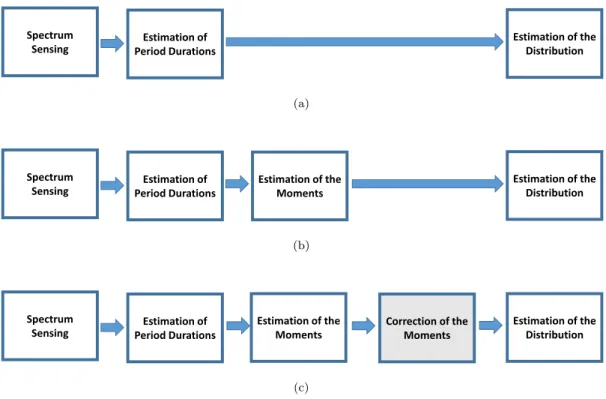
Sensing Period DurationsEstimation of

Estimation of the Distribution

(a)

Spectrum

Sensing Period DurationsEstimation of

Estimation of the Moments Estimation of the Distribution (b) Spectrum

Sensing Period DurationsEstimation of

Estimation of the Moments Correction of the Moments Estimation of the Distribution (c)

Figure 2.8: Distribution estimation methods : (a) Direct estimation, (b) Method of

Moments (MoM), (c) Modified Metod of Moments MMoM.

2.4.3 Considered Estimation Methods

Three methods are considered to estimate the distribution.

2.4.3.1 Direct Estimation

The direct estimation method is based on the calculation of the empirical cumulative distribution function (ecdf function in MATLAB). The ecdf function calculates the Kaplan-Meier estimate of the provided samples [100]. The flowchart of this strategy is illustrated in Fig. 2.8(a). The main drawback of this method is that the estimated distribution is discrete as the values of the estimated periods are integer multiples of the

sensing period (i.e., Tb_i =kT_s, k= 1,2,3, . . .). Moreover, it is not possible to apply any

correction factors to this estimation method, which affects its accuracy.

2.4.3.2 Estimation based on Method of Moments (MoM)

To overcome the first drawback of the direct estimation method, a solution based on the Method of Moments (MoM) is utilised. Instead of estimating the distribution of the PU activity periods directly from the observed periods themselves, which produces a discrete distribution, this method computes first the moments (mean and variance of the PU activity periods) and then estimates the parameters of the distribution based on the MoM assuming a certain distribution model. The flowchart of this strategy is illustrated in Fig. 2.8(b). The sample moments are equated to the distribution moments and then by solving the resulting equations the distribution parameters are obtained. As opposed to the previous method, the resulting distribution with this approach is continuous instead of discrete, thus offering the possibility to minimize the impact of sensing period.

Various methods have been proposed to estimate the distribution parameters besides MoM such as, Maximum likelihood Estimation and Least Squares Estimation [101, 102]. In this work, we only consider MoM-based solutions. Even though other methods might provide a better distribution parameters fit, they require the complete history of past observed period durations while with MoM the distribution moments can be estimated from sample moments, which can be computed recursively based on last samples. As a result, the practical implementation of MoM-based solutions would result in significantly lower computation and memory cost for CR devices.

Here, we assume the state holding times of PU (T0 and T1) follow a Generalized

Pareto (GP) distribution, which was proven to give best accuracy fit with a reasonable complexity in comparison with other more complex distributions [64]. The busy and idle durations are also assumed to be independent of each other [71]. The PDF and CDF for the GP distribution are given, respectively, as [94]:

fTi(t) =    0 t < µi 1 λi h 1 +αi(t−µi) λi i−(1/αi+1) t ≥ µi, (2.20) FTi(t) =    0 t < µi 1−h1 +αi(t−µi) λi i−1/αi t ≥ µi, (2.21)

whereαiandλi are the shape and scale of the GP distribution respectively, andµi is the location (also the minimum PU activity duration). Moreover, Ti ≥µi, αi ≥ 0, λi ≥0. The mean and variance of the GP distribution are expressed as:

E(Ti) =µi+

λi 1−αi

V(Ti) =

λ2_i

(1−αi)2(1−2αi)

. (2.23)

The expressions needed to estimate the parameters of the GP distribution from the sample moments can be obtained by solving (2.22) and (2.23) for such parameters, which yields: b µi= min(Tbi), (2.24) b αi = 1 2 1− (E(Tbi)− b µi)2 V(Tb_i) ! , (2.25) b λi = 1 2 1 + (E(Tb_i)−µ_bi)2 V(Tb_i) ! E(Tb_i)−µ_bi , (2.26)

wherebλ_i andα_bi are the estimated values of originalλ_iandα_i. Introducing the MoM

es-timates provided by (2.24), (2.25) and (2.26) into (2.20) and (2.21) provides a continuous estimation of the distribution of PU activity periods.

Notice that the location parameter µi can be estimated as shown in (2.24) since it corresponds to the minimum period duration. However, such estimation will be affected by the employed sensing period Ts. In many cases SU may be able to have a per-fect knowledge of this parameter, for example in the case of primary systems that use some form of regional beacon signals with real-time information [98] or when the radio technology of the primary system is standardised and known (e.g., the slot duration of GSM).

2.4.3.3 Estimation based on Modified Method of Moments (MMoM)

The MoM solution discussed in the previous section solves the problem of the estimation error introduced by the discrete distribution resulting from the direct estimation method. However, as shown in the analysis of Section 2.4.2, the estimated moments may have an error component resulting from the use of a finite sensing period Ts. This motivates the introduction of a Modified Method of Moments (MMoM) solution. The flowchart of this proposed strategy is illustrated in Fig. 2.8(c). The main difference with respect to the MoM method is the correction of the estimated moments, which is shaded in Fig. 2.8(c)

Based on (2.19), the new distribution parameters can be estimated as follows:

e αi = 1 2 1− (E(Tbi)−µ_bi)2 V(Te_i) ! , (2.27) e λi = 1 2 1 + (E(Tb_i)−µ_bi)2 V(Tei) ! E(Tb_i)−µ_bi . (2.28)

Notice that (2.27) and (2.28) are similar to their counterparts in (2.25) and (2.26), respectively, but are based on a corrected version of the moments. In particular, the