Towards Optimizing WLANs Power Saving: Novel
Context-Aware Network Traffic Classification
Based on a Machine Learning Approach
AHMED SAEED AND MARIO KOLBERG, (Senior Member, IEEE)
Department of Computing Science and Mathematics, Faculty of Natural Sciences, The University of Stirling, Stirling FK9 4LA, U.K.
Corresponding author: Ahmed Saeed ([email protected])
ABSTRACT Energy is a vital resource in wireless computing systems. Despite the increasing popularity of wireless local area networks (WLANs), one of the most important outstanding issues remains the power consumption caused by wireless network interface controller. To save this energy and reduce the overall power consumption of wireless devices, most approaches proposed to-date are focused on static and adaptive power saving modes. Existing literature has highlighted several issues and limitations in regards to their power consumption and performance degradation, warranting the need for further enhancements. In this paper, we propose a novel context-aware network traffic classification approach based on machine learning (ML) classifiers for optimizing WLAN power saving. The levels of traffic interaction in the background are contextually exploited for application of ML classifiers. Finally, the classified output traffic is used to optimize our proposed context-aware listen interval power saving modes. A real-world dataset is recorded, based on nine smartphone applications’ network traffic, reflecting different types of network behavior and interaction. This is used to evaluate the performance of eight ML classifiers in this initial study. The comparative results show that more than 99% of accuracy can be achieved. This paper indicates that ML classifiers are suited for classifying smartphone applications’ network traffic based on the levels of interaction in the background.
INDEX TERMS 802.11, energy consumption, machine learning (ML), power save mode (PSM), traffic
classification, WLAN.
I. INTRODUCTION
In the last few years, IEEE 802.11 Wireless Local Area Networks (WLANs) have become one of the most popular technologies that play an integral role in our lives. In WLANs, wireless devices such as laptops, smartphones and tablets are equipped with the Wireless Network Interface Controller (WNIC). WNIC allows wireless devices to share, commu-nicate and access information wirelessly through an Access Point (AP) [1]. One of the most important outstanding issues reaming in WLANs is the power consumption caused by WNIC during its communication with an AP. The high level of power consumption during the communication of WNIC directly affects the battery life of a wireless device, if is not connected to a power outlet [2].
To save energy caused by WNIC and reduce the overall power consumption of wireless devices, the 802.11 stan-dard defined a Static Power Save Mode (SPSM). In SPSM, a WNIC of a wireless device can sleep to save energy,
and wakes up periodically to receive its buffered packets from an AP [3].
The study of the existing literature [8]–[10] highlights several issues within SPSM, such as the overhead added by PS-Poll frames and delay of 100 to 300ms when the WNIC is off between the beacon intervals; this affects the performance of interactive applications such as web browser and real-time traffic of voice and video applications [12], [13].
To overcome the associated issues of SPSM, Adaptive PSM (APSM) has been deployed in the latest generation of mobile devices. APSM [7], [14] eliminates the delay of 100 to 300ms when the WNIC is off between beacon intervals, and the overhead caused by PS-Poll frames. However, the APSM does not consider the type of network traffic. As the WNIC switches from sleep to awake mode based on network activity thresholds. This may trigger the WNIC to be switched into awake mode unnecessarily in order to receive unimportant traffic and waste energy.
To eliminate the issue of the threshold mechanism built in APSM, Smart Adaptive PSM (SAPSM) proposed in [7]. Unlike SPSM and APSM which have been commercially deployed, SAPSM is still a research topic. SAPSM labels each network based application of smartphone into two set of priorities; high and low, with aid of a Machine Learn-ing (ML) classifier. SAPSM replaced the threshold mech-anism of APSM with set of two priorities, high and low. Thus for applications set as high priority, the WNIC will be adaptively switched into awake mode, and stays in the SPSM with applications set as low priority. No further modes have been considered in SAPSM for applications that afford to stay in a lower mode than SPSM. For example, applications that receive network updates after longer periods of time and or applications with buffer streaming.
This paper builds on SAPSM and provides a comprehen-sive study of classifying smartphone applications’ network traffic based on levels of interaction in the background, and proposes a new machine learning based approach to classify network traffic of wireless devices in WLANs. The lev-els of traffic interaction in the background are contextually exploited for the classification. The following contributions have been reported in this paper:
• The evaluation study applied to the smartphone applications network traffic, reflecting different levels of interaction in the background of each application.
• Nine selected smartphone applications depicting dif-ferent levels of interactions in the background; includ-ing, two VoIP applications, two applications of video calls, two applications of varied network interaction, two applications of very low network interaction, and finally one application representing applications with buffer streaming.
• Real-time instances of the nine selected applications
were captured, resulted in a construction of a novel dataset of 1350 instances, with 6 features per instance, named as Dataset 1.
• Further datasets were constructed by the application of different feature selection algorithms, Dataset 2CBFS is based on consistency feature selection algorithm and Dataset 3IGFS is based on information gain feature selection algorithm.
• Finally, eight ML classifiers were applied to three datasets and evaluated in terms of classification accu-racy, precision, recall, f-measure and processing time to build a classification model.
The rest of the paper is organized as follows. Section II reviews related work, specifically commercialized and state-of-the-art WLAN power saving protocols and approaches reported in the literature. This is followed by a review of internet traffic classification approaches, including machine learning approaches. Section III describes the data col-lection methodology employed in this study and the pro-posed framework. In particular, levels of traffic interaction in the background are exploited to provide contextual inputs for machine learning-driven network traffic classification.
Section IV presents simulation results and discussion. Finally, Section V outlines conclusions and future research directions.
II. RELATED WORKS
This section initially reviews existing power saving pro-tocols that are being commercially deployed in WLANs, specifically SPSM and APSM approaches, their comparative limitations and further developments in the area. This is fol-lowed by a critical overview of state-of-the art power saving approaches reported in the scientific literature.
A. REVIEW OF COMMERCIALIZED POWER SAVING PROTOCOLS
1) STATIC PSM
The SPSM in the infrastructure Basic Service Set (BSS), where each of wireless devices is connected to AP, the WNIC of a wireless device will be in one of these two modes, awake mode or sleep mode. In the awake mode, the wireless device is fully powered and is ready to transmit or receive; in con-trast, the wireless device in sleep mode is not fully powered and consumes very low power, and also cannot transmit or receive [4].
Thus, in SPSM the wireless device remains in sleep mode, and periodically wakes up from a time to another in order to listen for the Traffic Indication Map (TIM) in the beacon frame. The AP broadcasts the presence of any buffered pack-ets that destined to wireless device through a TIM in a beacon frame. If TIM indicates the presence of buffered packets for the wireless device, the wireless device remains awake and sends PS-poll frames requesting its buffered packets from the AP [5].
The awake wireless device keeps requesting for the buffered packets from the AP till all the packets are received, and AP indicates to a wireless device no there is no more buffered packets are left, then the wireless device goes back to sleep mode. A listen interval is the time interval which a wireless device wakes up periodically and listens to TIM. The listening interval is a multiple of the beacon interval. An example of 802.11 SPSM in infrastructure network is illustrated in Fig. 1.
So, the Wireless device wakes up and turning on its receiver in the listen interval to listen for TIM, TIM which sent by AP through beacon frame indicates that, the AP has no any buffered packet for the wireless device, so the wireless device immediately goes back into sleep mode, and skips the following beacon, because the listen interval is a multiple of beacon interval. Now again the wireless device wakes up and listen to the third beacon interval, this time the TIM indicates the presence of buffered packets for the wireless device in the AP.
Now, the wireless device sends a PS-Poll frame to AP requesting its buffered packets, these PS-Poll frames are sent by the wireless device according to Carrier Sense Multiple Access with Collision Avoidance (CSMA/CA). AP receives
FIGURE 1. Static PSM.
the Poll-Frame from the wireless device and then starts trans-mitting the buffered packets one by one, (transmits one packet and receives its corresponding ack frame from the wireless device and so on).
So the wireless device keeps sending the PS-Poll frames till the value of more data field in the data frame set to zero, which means there are no more packets buffered in AP for the wireless device [6].
2) ADAPTIVE PSM
To overcome the latency issues of the SPSM, APSM has been implemented in last generation of mobile devices. With APSM, mobile device switches between sleep to awake mode only if there is network traffic.
The WNIC does not take in consideration the type of network traffic whereas this type of network traffic is important or not, instead it switches from sleep to awake mode based on network activity thresholds. Thus, this enables WNIC to be switched into awake mode unneces-sarily in order to receive unimportant traffic and waste the energy [7].
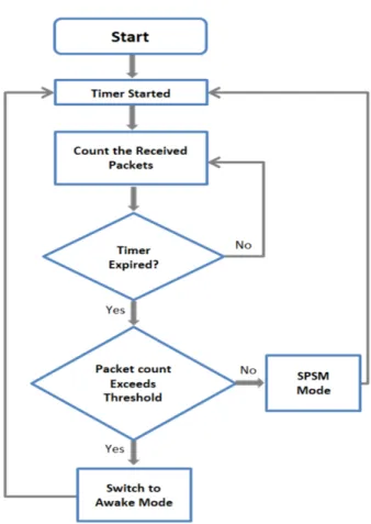
To switch from the sleep mode or vice versa, a null frame with power field disabled is sent to the AP, upon receiving this null frame, the AP stops buffering the packets for this wireless device. Now if a wireless device wants to switch back to the SPSM, then it sends a null frame but this time with power field enabled. So the AP starts buffering the packet for the wireless device. The threshold technique of APSM is shown in Fig. 2, where the frames are counted immediately after the timer start time and before the timer expiry time. If the number of counted packets exceeds the threshold, then WNIC switches to the awake mode, in case the number of counted fames less than the threshold, then WNIC switches back to SPSM [8].
FIGURE 2. Threshold mechanism of APSM.
3) LIMITATIONS AND FURTHER DEVELOPMENTS
The original mechanism of power saving mode that built into 802.11 standard, has several issues which leads to power con-sumption and performance degradation issues. For example, even in the power saving mode, the wireless device lasts for
long in the transmitting or awake state while the PS-Poll frames are sent to AP in order to retrieve the buffered frames once at a time from the AP [9], [10]. Nevertheless, the SPSM adds delay of 100 to 300ms when the WNIC of a wireless device is off between the beacon intervals, this delay impacts and causes issues regarding performance on both interactive applications such as web browsers and real-time applications such as VoIP [11]–[13].
The APSM eliminates the both issues in SPSM, the added delay of 100 to 300ms when the WNIC is off between the beacon intervals, and the overhead caused by PS-Poll frames, but, the WNIC does not take in consideration the type of network traffic whereas this type of network traffic is important or not, instead it switches from sleep to awake mode based on network activity thresholds. Thus, this enables WNIC to be switched into awake mode unnecessarily in order to receive unimportant traffic and waste the energy [7], [14]. An enhanced version of Automatic Power Save Delivery (APSD) mode been introduced in 802.11n, called Power Save Multi Poll (PSMP) mode which has two modes, Unscheduled PSMP (U-PSMP) and Scheduled PSMP (S-PSMP).
In U-PSMP, the wireless device informs the AP to buffer all the frames destined to the wireless device, and deliver these frames only when the AP sees a frame coming from that wireless device. Thus a frame coming from the wireless device acts like a trigger which allows the AP immediately transmitting frames to the wireless device [15].
With S-PSMP, AP sends schedules to wireless devices con-taining information about the time they are going to receive frames, so wireless devices go to sleep for the rest of time and awake only at the time determined on schedules [16].
The problem with PSMP is that, frames will be buffered for longer period of time at the AP which might also cause buffer overflow and packet loss.
Another mechanism that is concerned with antennas, called Spatial Multiplexing Power Save (SMPS) also has been intro-duced in 802.11n, which allows the wireless device to power down all of the receiving chains except one, but the problem with this mode, is that, the reduced number of receiving chains leads to less overall performance gained [10].
The Multiple Input Multiple Output (MIMO) antenna technique which was first introduced in 802.11n and further enhanced in 802.11ac, provides redundancy by using multi-ple antennas through spatial diversity, and provides higher bitrates through spatial multiplexing which allow multiple antennas to send independent information through each spa-tial path.
Despite the benefits of this technique (MIMO), this has significant implications in terms of energy consumption as the recent standard 802.11ac supports the use of 8 spatial streams [17], [18].
B. STATE-OF-THE-ART LITERATURE REVIEW
This section outlines and critically reviews a number of key power saving approaches reported in the scientific literature.
1) AP SIDE
He and Yuan [19] developed a time slicing PSM called scheduled PSM, which divides the period of beacon frame into multiple time slices. Buffered data are assigned to each time slices by the AP. They have redesigned the structure of TIM so it holds the slice assignment information. To avoid channel accessing issues, the TIM indicates all the relevant information about buffered data for the wireless device, so the wireless device knows if it has any buffered data assigned to it, if yes then also knows the delivery procedure. Thus during the time slicing for other wireless devices, it goes to sleep mode and save energy. The proposed technique by He and Yuan [19] reduces the energy consumption as there is no any channel contention, but if any wireless device does not wake up during its time slot, the time slot will be wasted. Also, He and Yuan [19] did not consider the packet length or the load of traffic with the time slots, all the time slots have the same length, thus the allocated time slot could be used inefficiently of light traffic.
Kwon and Cho [20] proposed simple priority scheme inter-user QoS. In this proposed scheme, the priority of each wire-less device is already defined. So the AP retrieves the user profile information from the Authentication, Authorization and Accounting (AAA) server upon the registration of the wireless device. Thus after determining the priority for each of wireless device, the wireless device with high priority is allowed to send the PS-POLL frames to retrieve its buffered packets immediately and earlier than wireless device which has been assigned as low priority. Thus the high priority device goes to sleeping mode for the rest of the beacon interval. Wireless devices set with the same priority levels are contended to access channel according to the Distributed Coordination Function (DCF) scheme. However the proposed scheme is only beneficial and in the favor of high priority wireless devices, as high priority wireless devices can fetch their buffered packets faster with minimal delay. But caus-ing delay and energy consumption for low priority wireless devices, as they keep sensing the channel till other wireless devices with higher priorities finish capturing their buffered packets from the AP.
Agrawal et al. [21] proposed Opportunistic Power Save Mode (OPSM) that operates well in a certain scenario such as short file downloads with short durations of think times in between two downloads. The authors observed that, the per-formance of wireless devices in SPSM is degraded when there are many numbers of wireless devices associated to an AP, which also leads to more power consumption. Thus in the proposed OPSM, the wireless device goes back to sleeping mode when the AP serving other wireless device, in other words, the wireless device waits for the opportu-nity to download its file with least energy consumption, when AP is not serving any of wireless devices. The one added bit in beacon frames which is transmitted periodi-cally by the AP, informs the wireless device that whether the AP is currently serving any other wireless devices or not.
To address the problem of wireless devices keep waking up during the communication of other wireless device with an AP. Omori et al. [22] proposed a PSM where wireless devices can sleep during Network Allocation Vector (NAV) period set by Request To Send/Clear To Send (RTS/CTS) handshake, to preserve delay the NAV duration is extended to allow burst transmission. If a wireless device overhears RTS or CTS is not destined to it, the wireless device goes to sleep during the NAV which is set by the RTS or CRT. Thus saves power by being sleep for the NAV duration. In order to address the energy consumption in exchanging the RTS/CTS packets, multiple packets are transmitted at a burst to wireless device by extending the NAV period set by RTS/CTS hand-shake. As multiple packets been transmitted at a burst to a wireless device, packets to other wireless devices will not be transmitted. To avoid delay of other wireless devices’ packets, the numbers of packets sent in burst transmission are adapted based on acceptable delay of each packet.
To reduce the number of wake-up listening intervals of a wireless device. This is a case when a wireless device wakes-up during its listen interval, turns on its WNIC and find no buffer packets for it in AP. Rozner et al. [8] presented a Network Assistant Power Management solution (NAPman) which is deployable through the AP. In this work they firstly have conducted experiments on APs and SPSM wireless devices to prove high level of energy consummation. Then they presented energy-aware fair scheduling algorithm in the First Come First Served (FCFS) manner, which applied only to packets of awake wireless devices. To avoid any con-tention, NAPman leverages virtualization, where one phys-ical AP acts as multiple virtual APs, thereby, each wireless device is isolated from another during downloading or fetch-ing packets from AP. But their approach can cause long delay for SPSM wireless device with much power left. Another limitation regarding to the virtualization is that, only very few number of virtual APs can be created with one physical AP. For example, Atheros chipset allows only up to 4 virtual APs to be created.
2) CLIENT SIDE
To reduce the number of wake-ups listening intervals of a wireless device, Li et al. [23] proposed a dynamic listen interval (DLI). Thus, in this scheme if a wireless device wakes up and finds no buffer packets for it at an AP, then the value of listen interval will be increased by one. In case, a wireless device wakes up and finds that there are buffered packets in AP. The value of the listen interval will be reset to the original value of listen interval during the SPSM. The proposed scheme might conserve energy of a wireless device comparing to the SPSM in term of increasing the sleeping time of a wireless device. But more delay will be added to the buffered packets belonging to interactive and VoIP applications when the listen interval is increased.
Pyles et al. [7] proposed SAPSM, which labels each network based application as high or low priority with aid of a ML classifier. SAPSM set each application with
a priority, so the application’s network traffic will be adap-tively switched to awake mode when the priority of an appli-cation is set to high. In contrast, appliappli-cation’s network traffic will not be switched to awake mode and remains in SPSM when the priority of an application is set to low. To train the classifier, Pyleset al.[7] conducted a user study where users have interacted with range of applications that have varied network patterns. After observing the usage patterns of an application, a comparison has taken place between these existing usage patterns and the usage patterns learned from classifier, and then the priority is estimated with minimal user intervention. When the priority is determined, the SAPSM stays in SPSM for low priority applications transmitting net-work data, and switches to awake mode when high priority applications transmitting network data.
In SAPSM, there is no priority for applications that can operate in lower mode than SPSM. Pyleset al.[7] imple-mented the technique by replacing the threshold method of APSM with high and low priorities, thus for high priority application the WNIC will be switched into awake mode while with low priority application will be switching into SPSM. Therefore, another mode must be considered for applications that afford to stay in a lower mode then SPSM. In other words, the sleeping time of a wireless device must be increased with applications that have network updates between long periods.
Liet al.[24] proposed a measurement based prioritization scheme which is motivated from SAPSM [7]. The proposed scheme is an online solution that prioritizes applications on smartphones. The main contributions of their work can be summarized as follows: Firstly, they have conducted mea-surements for application usage for the period of 6 weeks on smartphone; these measurements of the application usage were based on SystemSens. Based on measurement results, two key features have been extracted from netlog, receiving rate and screen touch rate. These two features are used to enhance the accuracy of prioritization scheme as well as reflecting the network interactivity. Based on the two selected features, the authors proposed an online solution that priori-tizes applications on smartphones. The demonstrated results shown that, the proposed scheme can prioritize applications based on two set of priorities only, high and low and conserve power most of the time.
C. REVIEW OF INTERNET TRAFFIC CLASSIFICATION APPROACHES
1) OVERVIEW
Traffic analysis is critical for evaluating and analyzing the performance of the networks, depending on the usage of the resources. The fundamental reason for analyzing the traffic of network is to assess the quality of service, trou-bleshoot the problems, and maintaining the overall security of the network [25]. Network classification is vital for ser-vice providers for managing the overall performance of the network, including certain aspects like Intrusion Detection
Systems (IDS) etc. For classifying the network on bigger scale and to understand which type of applications move within the network, another method is proposed named machine learning method [26]. With the technology moving towards cell phone and mobile phone applications, traffic classification has become even more important in the present era.
2) IMPORTANCE OF TRAFFIC CLASSIFICATION
Network traffic classification is important for identifying issues such as bandwidth, resource provisioning and the efficient usage of network resources [27]. The purpose of ML classifiers discussed by Al-Naymatet al. [28], suggests building a model consisting of classified instances and then using those instances for future classification, as accurately as possible. Traffic classification technology has gained sub-stantial importance of maintaining the quality of service implementation, book-keeping, and billing services as well as for managing security and network [29]. It is also found that the ML techniques are used vividly and can be con-sidered a vital aspect of the classification of internet traf-fic [30]. The importance of network traftraf-fic analysis also deals with customer services, overall bandwidth consumption of users, application of security rules, developing counteracting accounting and billing issues [31].
3) TRAFFIC CLASSIFICATION TECHNIQUES
IP network traffic classification has become a wide area of research with the substantial increase in the usage of internet. Traditional network traffic classification techniques; i.e. port based and payload based traffic classification techniques, suffer from a number of drawbacks [32]. In a port based technique, classification performed based on port numbers assigned by Internet Assigned Numbers Authority (IANA). Modern P2P applications have no standard port numbers [33]. Or other ports might be assigned to an application in order to avoid restrictions of some of the operating systems.
Payload based traffic classification, eliminates issues in the reliance on port numbers. By checking the payload of IP packet and matching the signature in the payload of each packet with the well-known signatures. Application of payload technique is ineffective with encrypted traf-fic; furthermore, significant computational cost is generated when payload classification technique is applied [34].
The area of the present research deals with such ML clas-sification that does not include the inspection of the packet payload data [31]. ML classification methods are used widely and are also investigated deeply.
Qin et al.[35] suggest that there are four possible steps for conducting traffic classification, first one is to define the important features of the network such as, packet lengths, packet interval of arrival, constructing a ML model, training the model to attain the level of classification required, and usage of the designed model to identify the unidentified flow of traffic in the classification system.
D. MACHINE LEARNING CLASSIFICATION OF SMART PHONE APPLICATIONS
A ML technology researched by Zhaoet al. [36] and proposed RobotDroid, which is based on Support Vector Machine (SVM) algorithm. The proposed framework detects unknown malware attacks on smartphones and mainly focuses on the disclosure of the confidential information, like private infor-mation of the users, payment/sales related inforinfor-mation, etc.
On the other hand, Stöberet al.[37] suggest a scheme in order to identify the network by utilizing the characteristics of the traffic patterns coming from the devices. The research also suggested that the 70 percent of the traffic belongs to the activities that are running in the background; hence, creating fingerprints by using those activities. By creating those fin-gerprints, the model can compare the incoming traffic from the fingerprints and then identifying the network traffic.
Another research, conducted by Taylor et al. [38] has suggested the alternative method in which a system is used to identify smartphone applications, which are encrypted through 802.11 frames. They gather data from the researched applications by running them vigorously and training them to classify the traffic by using the encrypted frames.
Similarly, Pyleset al.[7] employed SVM to classify the background traffic of number of applications, with the appli-cation of 6-folds cross-validation technique. The resultant maximal value of accuracy reported by them for SVM clas-sification model was 88.1%.
E. REVIEW OF MACHINE LEARNING ALGORITHMS
The main goal of ML is to construct a computer system that can adapt and learn from its experience. Each instance of a dataset used by ML algorithm is presented with the same set of features. If instances are labeled to the output class then this is called supervised. In contrast with unsupervised, instances are unlabelled. So the clustering algorithms will be applied in order to find unknown but useful categories of items [39]. This section reviews the eight commonly used ML that have been employed in this study.
1) MULTILAYER PERCEPTRON (MLP)
MLP is a feed forward neural network based model which consists of three different layers of nodes or neurons linked to each other, these layers are input, output and hidden layers. In MLP a set of input(s) data is mapped or assigned to a set of right output(s). For the purpose of training the net-work, the error signal of the output between the actual and desired, is propagated between the three layers in backward direction [40].
2) NAÏVE BAYES
Naïve Bayes is a classifier that is based upon probabilistic Bayes’ theorem; the classifier does not relate one attribute of a class to another for the assumption. Each attribute of class is independently linked to the parent class. Fig. 3, shows the simple formation of Naïve Bayes, the main class,
FIGURE 3. Naïve bayes.
and A, B and C are the features; there is no any other connec-tion between one attribute and other to the class [41].
3) DECISION TREE C4.5
The concept of decision tree classifier is to build a model based on a tree formation. Thus in this ML algorithm a certain attribute or feature is chosen in order to divide its samples into subsets. It is based upon the criteria of maximizing Standard Deviation Reduction (SDR). The attribute with highest SDR is chosen for each node and the decision will be processed. The same procedure will be repeated to smaller subset [42].
4) SUPPORT VECTOR MACHINE (SVM)
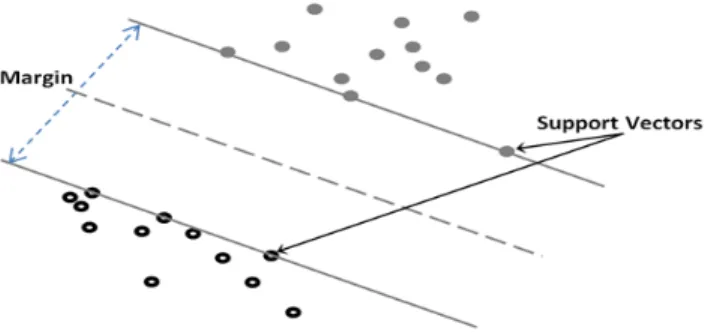
SVM classify data points into two categories by constructing optimal separating hyper plane which maximize the margin between data points of classes. Fig. 4 shows support vectors which are the points at boundaries, while the maximized mar-gin between data points of classes is shown in the middle [43].
FIGURE 4. SVM.
5) BAYES NET
Using Directed acyclic graphs (DAG), Bayesian network is a probabilistic model which can model variables as well as their conditional and or unconditional dependencies. For example: using input features classifying into the different types using the conditional dependencies of the input data. Bayesian networks are directed acyclic graph, whose nodes are the Bayesian structures, i.e. latent variables, hypothesis. From this the Bayesian network whose edge represents the conditional dependencies is associated with a probability function to which class the input variables belong [44].
6) RADIAL BASIS FUNCTION (RBF)
Using radial basis function as activation functions which uses distance from the origin point as a threshold metric, a neural network can be trained which is called radial basis function network. For example, some selected inputs work as radial basis kernels which together make a classification boundary, and whenever a new input arrives the distance weighted kernels make the decision class. Despite being single layered networks Radial Basis Functions Networks are a first step towards deep artificial neural network [45].
7) RANDOM FOREST
Random forest is a combination of many decision trees and considered an ensemble learning method, which uses mul-tiple decision trees to classify and correct the over-fitting problem created by a unit decision tree alone. For exam-ple, using only some of the input features into a tree and other features into another tree can then be ensembled into a greater and robust classifier using Random forest. The Random Forest is a third stage in the tree, bagging of tree and forest pipeline [46].
8) k-NEAREST NEIGHBOR (KNN)
KNN is a non-parametric (without using any hyper parame-ters as input to the network) classification method. In which the input is given k closest hyper dimensional vectors in the feature space, and the output is achieved using highest occur-rence of the classes. In an abstract sense, this algorithm is a voting system in which the nearest hyper dimensional vectors form a classification inference on the input raw data [47].
F. OTHER RECENT DEEP LEARNING ALGORITHMS
More recently deep learning approaches have been reported in [48] and [49]. For example, the Convolutional Neural Network (CNN) is widely used in deep neural networks. Compared to the MLP model, CNN adds more convolu-tion layers; there are a number of steps being processed in the convolutional layer. I.e. transforming the input into two dimensional arrays, then applying a sliding window which has the weight vector of the two dimensional to the input. Lastly, the input which has processed is down-sampled by 2×2 matrixes [49].
III. DATA COLLECTION METHODOLOGY AND PROPOSED FRAMEWORK
This section describes the data collection methodology employed in this study. The dataset was constructed by capturing real-time background traffic of 9 applications. Table 1 shows the chosen applications and the degree of network interactivity in the background. All the applications including the NetworkLog installed from the official Google play store. 150 samples/instances of the network traffic in the background captured for each app with the aid of Network-Log, and the running time of 25 minutes resulted in a total of 1350 samples. Samsung Galaxy S5 is used to capture all the
FIGURE 5. Arrays of Network Behavior Characterized by Levels of Traffic Interaction. TABLE 1. Applications and the degree of network interactivity.
instances of the background traffic of the entire applications running Android version 6.0.1.
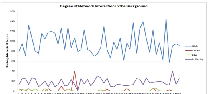
The 9 applications represent different types of network behavior in the background, for high level of network inter-action; we have considered video and voice calls of Skype and Google Hangouts. For the varied level of interactions Facebook and Gmail been chosen, for Gmail, 23 emails were received at random instances. And 23 tagged posts were received at random instances for Facebook as updates. NSS and NSC chosen to represent all applications with lower degree of interaction, these applications mostly are offline, the interaction occurred only during fetching advertise-ments. Finally to represent applications with audio buffering capability XiiaLive internet radio application considered, we chose a random station 128kbps stream.
The dataset has been labeled in accordance to the level of interactivity in the background of each application. Fig. 5 illustrates the receiving data rate in Kbytes/sec of the first 50 instances, based on the level of interaction in the background of the applications.
All inputs of applications with high and constant level of background interactivity are labeled as high. Inputs of applications of varied level of background interactivity were labeled as varied. Low was the label for the inputs of appli-cations with low level of interactivity, and we have labeled the samples of XiiaLive internet radio app with output class buffer.
The dataset with full number of six highly correlated fea-tures named as Dataset 1, table 2 shows the full set of feafea-tures extracted using NetworkLog form the background of each application.
TABLE 2.Full set of 6 features.
A. PROPOSED FRAMEWORK
1) CONTEXT-AWARE LISTEN INTERVAL (CALI)
The proposed methodology aims to optimize the efficiency of applications’ background traffic and WNIC. The WNIC
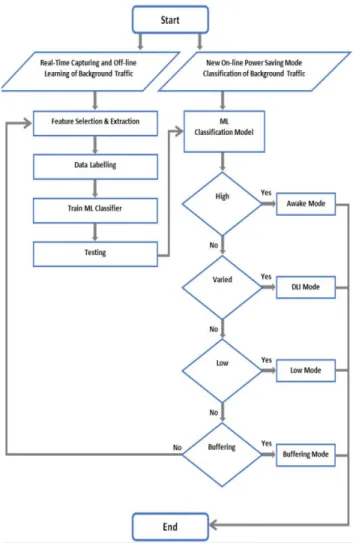
awakes and sleeps in accordance to the level of interactiv-ity in the background of each application. Current APSM eliminates only the latency issues of the SPSM, without considering the type of network traffic whereas this type of network traffic is important or not, instead it switches from sleep to awake mode based on network activity thresholds. Pyles et al. [7] introduced a system based on categorizing all types of applications into two categories; High and Low, this is again does not fulfill the urgent need of a system that consider the level of interactivity in the background of applications. CALI introduces the concept of context aware listen interval, where the WNIC of a wireless device, with the aid of ML classification model sleeps and awakes based on inputs received and transmitted by the WNIC. Equivalently, levels of traffic interaction in the background are used as contextual inputs for training ML classifiers of output traffic. Finally, the classified output traffic is used to optimize CALI power saving modes, proposed in the next section.
Fig. 6, shows the flowchart of the proposed framework, where real-time instances of background traffic of each appli-cation are captured and labeled to the right output class/mode. Instances of applications with higher level of background interactivity are labeled as high, e.g. video and voice calls.
FIGURE 6. Context-aware listen interval.
Instances of applications with varied level of interactivity are labeled as varied, e.g. Facebook and Gmail. Instances of applications with lower level of interactivity are labeled as low, e.g. NSS and NCS. Furthermore, CALI also considers applications with buffer streaming capability, e.g. the samples of XiiaLive internet radio app are labeled as buffering.
The input samples of each application are labeled to the correct output class based on the level of interactivity and controlled experiments. The labeled samples are trained and validated by the ML classifier, in order to build the ML classi-fication model. Subsequently the ML classiclassi-fication model is capable to identify the new unseen samples and classify them accordingly, e.g. ML classification model assigns samples of highly interactive application to the class high in accordance with the training accomplished in the previous step. In the next section, a number of CALI power saving modes are proposed to optimize efficiency of our envisaged WLAN power saving framework.
2) PROPOSED CALI POWER SAVING MODES
Four CALI power saving modes are employed, as illustrated in the examples below:
When the background samples of highly interactive appli-cations classified to the output class high with the aid of ML classification model, the application is set to high, so the listen interval will be adjusted to awake mode.
ML classification model classifies the background samples for applications with the varied level of interactivity to the DLI mode. We have considered DLI mode proposed in [23] with an upper bound 8= 800ms in DLI mode, the listen interval is increased by 1 each time when there is no interac-tion in receiving data in the background. And rest to 1 when interaction occurs. Applications, e.g. Gmail and Facebook not always send or revive data, thus assigning them with an awake mode is not as an efficient option.
Based on observations and controlled experiments, inter-action in the background for applications e.g. NSS and NCS occurs during fetching advertisements only. Thus, for these types of applications the ML classification model is capable to classify their samples to the output class low. Therefore, the listen interval is forced to sleep for a defined longer time based on controlled experiments.
Finally, and based on observations and controlled exper-iments, audio streaming applications, e.g. XiiaLive internet radio app. Could be assigned to a mode that is capable to adjust longer sleeping time than a SPSM applied in [7]. As switching off the WINC for couple of seconds does not impact on the playback streaming quality.
B. FEATURES SELECTION AND EXPERIMENTAL SETUP
The main purpose of feature selection, is to minimize the set of features by eliminating any irrelevant and redundant features resulting in less computational complexity, higher classification accuracy and maximized generalization capa-bility [50], [51]. Therefore, to extract eliminated versions
of datasets, two widely used feature selections algorithms were considered.
1) CONSISTENCY BASED FEATURE SELECTION (CBFS) [52]
Evaluates all the subsets of features, in order to determine the smallest optimum subset of features, which is consistently capable to map to the output class as with full set of features.
2) INFORMATION GAIN FEATURE SELECTION (IGFS) [53]
Evaluates all the features with the output class, features with higher information gain value to the output class are selected. Best first search method was applied to attribute selection for CBFS algorithm, while ranker method was selected for IGFS algorithm.
Weka tool was used, for the extraction and the application of the reduced features’ datasets, named as Dataset 2CBFS, and Dataset 3IGFS. 1350 data samples were included in each set representing the total of 9 applications, the total number of six features included in Dataset 1, reduced number of 4 fea-tures were included in Dataset 2CBFS, and Dataset 3IGFS.
Table 3, shows the list of features after applying CBFS algorithm, while table 4 shows the list of features after apply-ing the IGFS algorithm, the top 4 features in rankapply-ing were chosen.
TABLE 3. Set of features for Dataset 2CBFS.
TABLE 4. Set of features for Dataset 3IGFS.
The experiments were performed with the aid of WEKA [54], a well-known ML tool, applied in many studies including [55], [56]. v3.6.12 on a desktop computer operating Microsoft windows 7 Enterprise with Intel core i7-4770 CPU of 3.40 GHz and 4 GB of RAM.
For validating the accuracy of ML algorithm in predicting/ mapping the inputs to the correct output class, and based on the recommendation of [57], cross validation of K=10 is used to avoid over-fitting and to see how well ML algorithms
perform in classifying the unseen samples. Thus, the dataset is divided into 10 N equal parts or portions, each portion (1/N) is used for testing, while the remaining ((N−1)/N) are used for training.
In order to determine the finest ML classifier, performance of the 8 ML classifiers defined in subsection II-E were ana-lyzed. Thus, the chosen ML classifiers are; Bayes Net, Naïve Bayes, SVM, MLP, RBF, KNN, Random forest and C4.5.
The performance of each classifier evaluated based on the following metrics:
Classification Accuracy:this is a percentage of samples or instances classified or mapped correctly to the class.
Precision: this is a proportion of instances which truly belonging to class A among all that classified to that class.
Recall:is equivalent to the True Positive Rate (TPR), it is a proportion of instances belonging to a particular class A and classified as class A.
F-measure:is a harmonic average that combines precision and recall.
IV. EXPERIMENTAL RESULTS AND ANALYSIS
This section, analyzes the performance of the eight ML classifiers on Dataset 1, Dataset 2CBFS and Dataset 3IGFS, in terms of classification accuracy, precision, recall and f-measure.
Fig. 7 shows the performance of the 8 ML classifiers based on the classification accuracy on each of the 6 features applied in this study. The classification accuracies of the eight ML classifiers were increased with the complete set of 6 features Dataset 1 as shown in Fig 8. Thus, the highest classification accuracy was achieved by Random Forest of 99.48%. Naïve Bayes produced the lowest classification accuracy of 93.25%. Bayes Net, RBF, KNN and C4.5 achieved the classification accuracy of more than 98%.
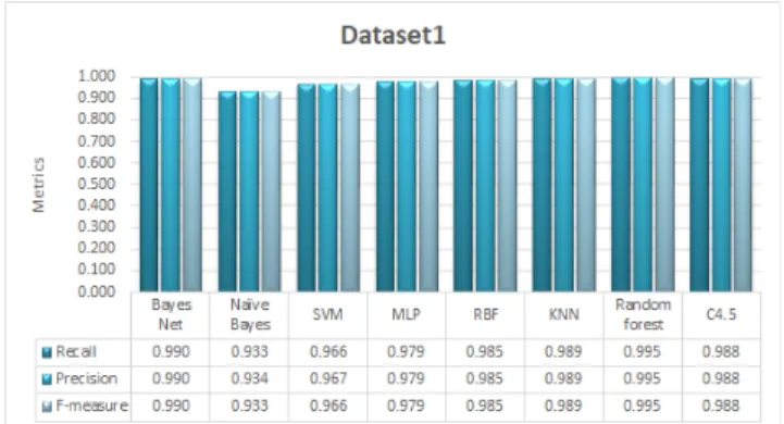
In terms of recall, precision and f-measure values of the 8 ML classifiers on Dataset 1, Fig. 9 shows Random Forest attained the highest values of 0.995 among all other classifiers. Recall, precision and f-measure values of 0.933, 0.934 and 0.933 for Naïve Bayes were the lowest among all other classifiers.
Classification accuracy of the 8 ML classifiers on the reduced set of 4 features dataset 2CBFS; with the application of best first search method and consistency based feature selection technique is represented in Fig. 10.
The classification accuracy of Bayes Net, Naïve Bayes and RBF was increased as opposed to Dataset 1, with clas-sification accuracy of 99.03% for Bayes Net, 93.92% for Naïve Bayes and 98.74% for RBF. MLP produced the same classification accuracy of 97.85% as opposed to Dataset 1.
While, the classification accuracy for the rest ML classi-fiers decreased in dataset 2CBFS compared to Dataset 1.
Fig. 11 shows the comparison of recall, precision and f-measure values on dataset 2CBFS. The recall, precision and f-measure values of 0.990 for Bayes Net and 0.979 for MLP remain unchanged as opposed to Dataset 1. The recall, precision and f-measure values of Naïve Bayes and RBF were
FIGURE 7. Classification accuracy of ML Classifiers on Individual Feature.
FIGURE 8. Classification accuracy of ML classifiers on dataset 1.
FIGURE 9. Comparison of recall, precision and F-Measure on dataset 1.
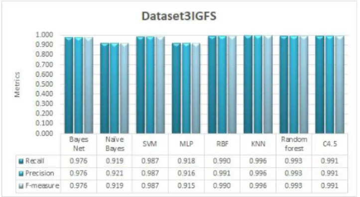
slightly increased as opposed to Dataset 1. While the metrics values of the rest of the ML classifiers slightly decreased in comparison to Dataset 1. Fig. 12 represents the Dataset 3IGFS, where the set of features extracted from the full set of 6 features using the information gain technique. The top 4 features were selected based on ranker method.
FIGURE 10. Classification accuracy of ML Classifiers on Dataset 2CBFS.
FIGURE 11. Comparison of recall, precision and F-Measure on dataset 2CBFS.
KNN achieved the highest classification accuracy of 99.62% in Dataset 3IGFS. SVM, RBF and C4.5 produced better classification accuracy of 98.66%, 99.03% and 99.11% compared to dataset 1 and dataset 2CBFS.
Furthermore, the classification accuracy of 99.33% for Random Forest was decreased compared to dataset 1.
FIGURE 12. Classification accuracy of ML classifiers on dataset 3IGFS. Finally, the classification accuracy of Bayes Net, Naïve Bayes and MLP was the lowest in Dataset 3IGFS compared to Dataset 1 and Dataset 2CBFS.
Fig.13 displays the comparison of recall, precision and f-measure values of the 8 ML classifiers on Dataset 3IGFS. The recall, precision and f-measure value of 0.996 was the highest in Dataset 3IGFS and was achieved by KNN. The metrics values of recall, precision and f-measure for Bayes Net, Naïve Bayes and MLP decreased in comparison to dataset 1 and dataset 2CBFS. SVM, RBF and C4.5 produced better values in terms of recall precision and f-measure com-pared to dataset 1 and dataset 2CBFS.
FIGURE 13. Comparison of recall, precision and F-Measure on dataset 3IGFS.
Table 5 shows the time taken by each of ML classifier in all datasets to build a ML classification model.
TABLE 5. Processing time to build the classification model (in seconds).
Narudinet al. [58] discussed, the time taken by classifiers to a build a model is very crucial and affects the resource
consumption of a wireless device. Thus, considering the pro-cessing time of classifiers to build a model is very important. The processing time of 0.01s for KNN and Naïve Bayes were the shortest time to build a model and remain identical in all datasets, while the processing time of 1.42 s for MLP to build a model in dataset 1 was the longest compared with all other classifiers in all datasets. The model building time for Bayes Net, SVM, MLP and Random forest decreased in Dataset 3IGFS when compared with Dataset 1 and Dataset 2CBFS. Finally, the processing time of 0.01 s for C4.5 remains iden-tical in Dataset 2CBFS and Dataset 3IGFS.
Comparing the results obtained for the eight ML classifiers in all datasets in terms of classification accuracy, we found a number of effective features must be considered to improve the overall classification accuracy. Moreover, we conclude that the optimum results in terms of all evaluation metrics used in this study was achieved by KNN in Dataset 3IGFS. We determined KNN to be the best ML classifier for our proposed CALI model, in terms of classifying smartphone applications’ network traffic based on levels of interaction in the background.
V. CONCLUSIONS AND FUTURE WORK
Despite the significant increasing popularity of WLANs, the level of power consumed by WNIC remains one of the most important outstanding issues. Existing literature has highlighted several issues and limitations within the commer-cialized power saving protocols, and approaches reported in the scientific literature. Pyleset al.[7] introduced SAPSM, which replaces the threshold mechanism of APSM with set of two priorities, high and low. Thus each network based application of smartphone labeled as high and low, with aid of a ML classifier.
Comparing to SAPSM, this work has extended the number of categories by considering a varied range of smartphone applications’ network traffic that reflect different levels of interaction in the background.
We proposed a new ML based approach to classify network traffic of wireless devices in WLANs. The levels of traffic interaction in the background are contextually exploited for the classification by the application of ML classifiers. Based on the evaluation results of eight ML classifiers, more than 99% of accuracy was achieved by Random Forest, Bayes Net, decision tree C4.5, RBF and the optimized accuracy of 99.62% was achieved by KNN.
As future work, we will consider the full implementation and evaluation of the proposed methodology, specifically of the proposed CALI power saving modes, and comparison with existing benchmark power saving approaches, includ-ing SPSM [6], APSM and SAPSM [7] in terms of power saving.
REFERENCES
[1] M. S. Afaqui, E. Garcia-Villegas, and E. Lopez-Aguilera, ‘‘IEEE 802.11ax: Challenges and requirements for future high efficiency WiFi,’’IEEE Wire-less Commun., vol. 24, no. 3, pp. 130–137, Jun. 2017.
[2] S. K. Saha, P. Deshpande, P. P. Inamdar, R. K. Sheshadri, and D. Koutsonikolas, ‘‘Power-throughput tradeoffs of 802.11n/ac in smartphones,’’ in Proc. IEEE Conf. Comput. Commun. (INFOCOM), Apr./May 2015, pp. 100–108.
[3] C. Monteleoni, H. Balakrishnan, N. Feamster, and T. Jaakkola, ‘‘Man-aging the 802.11 energy/performance tradeoff with machine learning,’’ MIT CSAIL, Cambridge, MA, USA, Tech. Rep. MIT-LCS-TR-971, 2004.
[4] R. Palacios, G. M. Mekonnen, J. Alonso-Zarate, D. Kliazovich, and F. Granelli, ‘‘Analysis of an energy-efficient MAC protocol based on polling for IEEE 802.11 WLANs,’’ in Proc. IEEE Int. Conf. Com-mun. (ICC), Jun. 2015, pp. 5941–5947.
[5] P. Swain, S. Chakraborty, S. Nandi, and P. Bhaduri, ‘‘Performance model-ing and analysis of IEEE 802.11 IBSS PSM in different traffic conditions,’’
IEEE Trans. Mobile Comput., vol. 14, no. 8, pp. 1644–1658, Aug. 2015. [6] IEEE 802.11-2012: Wireless LAN Medium Access Control MAC and
Phys-ical Layer PHY Specifications, IEEE Standard 802.11 LAN, 2012. [7] A. J. Pyles, X. Qi, G. Zhou, M. Keally, and X. Liu, ‘‘SAPSM: Smart
adaptive 802.11 PSM for smartphones,’’ inProc. ACM Conf. Ubiquitous Comput., Sep. 2012, pp. 11–20.
[8] E. Rozner, V. Navda, R. Ramjee, and S. Rayanchu, ‘‘NAPman: Network-assisted power management for WiFi devices,’’ inProc. 8th Int. Conf. Mobile Syst., Appl., Services, Jun. 2010, pp. 91–106.
[9] G. Anastasi, M. Conti, E. Gregori, and A. Passarella, ‘‘802.11 power-saving mode for mobile computing in Wi-Fi hotspots: Limitations, enhancements and open issues,’’ Wireless Netw., vol. 14, no. 6, pp. 745–768, Dec. 2008.
[10] S. Sudarshan, R. Prasad, A. Kumar, R. Bhatia, and B. R. Tamma, ‘‘Uber-sleep: An innovative mechanism to save energy in IEEE 802.11 based WLANs,’’ inProc. IEEE Int. Conf. Electron., Comput. Commun. Tech-nol. (IEEE CONECCT), Jan. 2014, pp. 1–6.
[11] S.-L. Tsao and C.-H. Huang, ‘‘A survey of energy efficient MAC protocols for IEEE 802.11 WLAN,’’Comput. Commun., vol. 34, no. 1, pp. 54–67, 2011.
[12] X. Pérez-Costa and D. Camps-Mur, ‘‘APSM: Bounding the downlink delay for 802.11 power save mode,’’ inProc. IEEE Int. Conf. Commun. (ICC), vol. 5, May 2005, pp. 3616–3622.
[13] Z. Zeng, Y. Gao, and P. R. Kumar, ‘‘SOFA: A sleep-optimal fair-attention scheduler for the power-saving mode of WLANs,’’ inProc. 31st Int. Conf. Distrib. Comput. Syst. (ICDCS), Jun. 2011, pp. 87–98.
[14] V. Bernardo, B. Correia, M. Curado, and T. I. Braun, ‘‘Towards end-user driven power saving control in Android devices,’’ in
Internet of Things, Smart Spaces, and Next Generation Networks and Systems. Cham, Switzerland: Springer, 2014, pp. 231–244. [Online]. Available: https://link.springer.com/chapter/10.1007/978-3-319-10353-2_20#aboutcontent
[15] X. Pérez-Costa and D. Camps-Mur, ‘‘IEEE 802.11E QoS and power saving features overview and analysis of combined performance [Accepted from Open Call],’’IEEE Wireless Commun., vol. 17, no. 4, pp. 88–96, Aug. 2010.
[16] D. A. Westcott, D. D. Coleman, B. Miller, and P. Mackenzie, CWAP Certified Wireless Analysis Professional Official Study Guide: Exam PW0-270. Hoboken, NJ, USA: Wiley, 2011.
[17] I. Pefkianakis, C.-Y. Li, and S. Lu, ‘‘What is wrong/right with IEEE 802.11n spatial multiplexing power save feature?’’ inProc. 19th IEEE Int. Conf. Netw. Protocols (ICNP), Oct. 2011, pp. 186–195.
[18] L. Verma, M. Fakharzadeh, and S. Choi, ‘‘WiFi on steroids: 802.11AC and 802.11AD,’’IEEE Wireless Commun., vol. 20, no. 6, pp. 30–35, Dec. 2013.
[19] Y. He and R. Yuan, ‘‘A novel scheduled power saving mechanism for 802.11 wireless LANs,’’IEEE Trans. Mobile Comput., vol. 8, no. 10, pp. 1368–1383, Oct. 2009.
[20] S.-W. Kwon and D.-H. Cho, ‘‘Efficient power management scheme consid-ering inter-user QoS in wireless LAN,’’ inProc. IEEE 64th Veh. Technol. Conf. (VTC-Fall), Sep. 2006, pp. 1–5.
[21] P. Agrawal, A. Kumar, J. Kuri, M. K. Panda, V. Navda, and R. Ramjee, ‘‘OPSM—Opportunistic Power Save Mode for Infrastructure IEEE 802.11 WLAN,’’ inProc. IEEE Int. Conf. Commun. Workshops (ICC), May 2010, pp. 1–6.
[22] K. Omori, Y. Tanigawa, and H. Tode, ‘‘A study on power saving using RTS/CTS handshake and burst transmission in wireless LAN,’’ inProc. 10th Asia–Pacific Symp. Inf. Telecommun. Technol. (APSITT), Aug. 2015, pp. 1–3.
[23] Y. Li, X. Zhang, and K. L. Yeung, ‘‘DLI: A dynamic listen interval scheme for infrastructure-based IEEE 802.11 WLANs,’’ inProc. IEEE 26th Annu. Int. Symp. Pers., Indoor, Mobile Radio Commun. (PIMRC), Aug./Sep. 2015, pp. 1206–1210.
[24] Y. Li, G. Zhou, G. Ruddy, and B. Cutler, ‘‘A measurement-based prior-itization scheme for smartphone applications,’’Wireless Pers. Commun., vol. 78, no. 1, pp. 333–346, Sep. 2014.
[25] G. Srivastava, M. P. Singh, P. Kumar, and J. P. Singh, ‘‘Internet traffic clas-sification: A survey,’’ inRecent Advances in Mathematics, Statistics and Computer Science. Singapore: World Scientific, 2016, p. 611. [Online]. Available: https://www.worldscientific.com/worldscibooks/10.1142/9651 [26] M. Shafiq, X. Yu, A. A. Laghari, L. Yao, N. K. Karn, and F. Abdessamia,
‘‘Network traffic classification techniques and comparative analysis using Machine Learning algorithms,’’ inProc. 2nd IEEE Int. Conf. Comput. Commun. (ICCC), Oct. 2016, pp. 2451–2455.
[27] J. Kaur, S. Agrawal, and B. S. Sohi, ‘‘Internet traffic classification for educational institutions using machine learning,’’Int. J. Intell. Syst. Appl., vol. 4, no. 8, pp. 37–45, Jul. 2012.
[28] G. Al-Naymat, M. Al-Kasassbeh, N. Abu-Samhadanh, and S. Sakr, ‘‘Classification of VoIP and non-VoIP traffic using machine learning approaches,’’J. Theor. Appl. Inf. Technol., vol. 92, no. 2, p. 403, Oct. 2016. [29] P. M. S. del Río, ‘‘Internet traffic classification for high-performance and off-the-shelf systems,’’ Ph.D. dissertation, Auton. Univ. Madrid, Madrid, Spain, May 2013.
[30] N. Namdev, S. Agrawal, and S. Silkari, ‘‘Recent advancement in machine learning based Internet traffic classification,’’ Procedia Comput. Sci., vol. 60, pp. 784–791, Jan. 2015.
[31] M. Soysal and E. G. Schmidt, ‘‘Machine learning algorithms for accurate flow-based network traffic classification: Evaluation and comparison,’’
Perform. Eval., vol. 67, no. 6, pp. 451–467, Jun. 2010.
[32] T. T. T. Nguyen and G. Armitage, ‘‘A survey of techniques for Internet traffic classification using machine learning,’’IEEE Commun. Surveys Tuts., vol. 10, no. 4, pp. 56–76, 4th Quart., 2008.
[33] A. Tongaonkar, R. Keralapura, and A. Nucci, ‘‘Challenges in network application identification,’’ inProc. LEET, Apr. 2012, p. 1.
[34] S. Valenti, D. Rossi, A. Dainotti, P. Pescapè, A. Finamore, and M. Mellia, ‘‘Reviewing traffic classification,’’ inData Traffic Monitoring and Analy-sis. Berlin, Germany: Springer, 2013, p. 123.
[35] D. Qin, J. Yang, J. Wang, and B. Zhang, ‘‘IP traffic classification based on machine learning,’’ inProc. IEEE 13th Int. Conf. Commun. Tech-nol. (ICCT), Sep. 2011, pp. 882–886.
[36] M. Zhao, T. Zhang, F. Ge, and Z. Yuan, ‘‘RobotDroid: A lightweight malware detection framework on smartphones,’’J. Netw., vol. 7, no. 4, p. 715, 2012.
[37] T. Stöber, M. Frank, J. Schmitt, and I. Martinovic, ‘‘Who do you sync you are?: Smartphone fingerprinting via application behaviour,’’inProc. 6th ACM Conf. Secur. Privacy Wireless Mobile Netw., Apr. 2013, pp. 7–12. [38] V. F. Taylor, R. Spolaor, M. Conti, and I. Martinovic, ‘‘Robust smartphone
app identification via encrypted network traffic analysis,’’IEEE Trans. Inf. Forensics Security, vol. 13, no. 1, pp. 63–78, Jan. 2018.
[39] S. Marsland,Machine Learning: An Algorithmic Perspective. Boca Raton, FL, USA: CRC Press, 2015.
[40] C. Zhanget al., ‘‘A hybrid MLP-CNN classifier for very fine resolution remotely sensed image classification,’’ISPRS J. Photogram. Remote Sens., vol. 140, pp. 133–144, Jun. 2018.
[41] Z. Wu, Q. Xu, J. Li, C. Fu, Q. Xuan, and Y. Xiang, ‘‘Passive indoor localization based on CSI and Naive Bayes classification,’’IEEE Trans. Syst., Man, Cybern., Syst., vol. 48, no. 9, pp. 1566–1577, Sep. 2018. [42] A. Subasi, M. Radhwan, R. Kurdi, and K. Khateeb, ‘‘IoT based mobile
healthcare system for human activity recognition,’’ inProc. 15th Learn. Technol. Conf. (L&T), Feb. 2018, pp. 29–34.
[43] A. Rosales-Perez, S. Garcia, H. Terashima-Marin, C. A. C. Coello, and F. Herrera, ‘‘MC2ESVM: Multiclass classification based on cooperative evolution of support vector machines,’’IEEE Comput. Intell. Mag., vol. 13, no. 2, pp. 18–29, May 2018.
[44] C. Premebida, D. R. Faria, and U. Nunes, ‘‘Dynamic Bayesian network for semantic place classification in mobile robotics,’’Auto. Robots, vol. 41, no. 5, pp. 1161–1172, Jun. 2017.
[45] I. Aljarah, H. Faris, S. Mirjalili, and N. Al-Madi, ‘‘Training radial basis function networks using biogeography-based optimizer,’’Neural Comput. Appl., vol. 29, no. 7, pp. 529–553, Apr. 2018.
[46] W. Lin, Z. Wu, L. Lin, A. Wen, and J. Li, ‘‘An ensemble random forest algorithm for insurance big data analysis,’’IEEE Access, vol. 5, pp. 16568–16575, 2017.
[47] S. Zhang, X. Li, M. Zong, X. Zhu, and D. Cheng, ‘‘Learningkfor kNN classification,’’ACM Trans. Intell. Syst. Technol., vol. 8, no. 3, 2017, Art. no. 43.
[48] N. Mehdiyev, J. Lahann, A. Emrich, D. Enke, P. Fettke, and P. Loos, ‘‘Time series classification using deep learning for process planning: A case from the process industry,’’ Procedia Comput. Sci., vol. 114, pp. 242–249, Oct. 2017. [Online]. Available: https://www.sciencedirect.com/science/article/pii/S1877050917318707 [49] U. R. Acharya, S. L. Oh, Y. Hagiwara, J. H. Tan, and H. Adeli, ‘‘Deep
convolutional neural network for the automated detection and diagnosis of seizure using EEG signals,’’Comput. Biol. Med., vol. 100, pp. 270–278, Sep. 2017.
[50] H. Peng, F. Long, and C. Ding, ‘‘Feature selection based on mutual infor-mation criteria of max-dependency, max-relevance, and min-redundancy,’’
IEEE Trans. Pattern Anal. Mach. Intell., vol. 27, no. 8, pp. 1226–1238, Aug. 2005.
[51] J. Liet al., ‘‘Feature selection: A data perspective,’’ACM Comput. Surv., vol. 50, no. 6, p. 94, Jan. 2017.
[52] L. Morán-Fernández, V. Bolón-Canedo, and A. Alonso-Betanzos, ‘‘Cen-tralized vs. distributed feature selection methods based on data complexity measures,’’Knowl.-Based Syst., vol. 117, pp. 27–45, Feb. 2017. [53] V. F. Rodriguez-Galiano, J. A. Luque-Espinar, M. Chica-Olmo, and
M. P. Mendes, ‘‘Feature selection approaches for predictive modelling of groundwater nitrate pollution: An evaluation of filters, embedded and wrapper methods,’’ Sci. Total Environ., vol. 624, pp. 661–672, May 2018.
[54] Weka Website. Accessed: Oct. 11, 2018. [Online]. Available: http:// www.cs.waikato.ac.nz/ml/weka/
[55] L. Verde, G. De Pietro, and G. Sannino, ‘‘Voice disorder identifi-cation by using machine learning techniques,’’ IEEE Access, vol. 6, pp. 16246–16255, 2018.
[56] S. B. Sakri, N. B. A. Rashid, and Z. M. Zain, ‘‘Particle swarm optimization feature selection for breast cancer recurrence prediction,’’IEEE Access, vol. 6, pp. 29637–29647, 2018.
[57] R. Kohaviet al., ‘‘A study of cross-validation and bootstrap for accuracy estimation and model selection,’’ inProc. Int. Joint Conf. AI, Aug. 1995, vol. 14, no. 2, pp. 1137–1145.
[58] F. A. Narudin, A. Feizollah, N. B. Anuar, and A. Gani, ‘‘Evaluation of machine learning classifiers for mobile malware detection,’’Soft Comput., vol. 20, no. 1, pp. 343–357, 2016.
Authors’ photographs and biographies not available at the time of publication.