Point and Interval Forecasting of Spot
Electricity Prices: Linear vs. Non-Linear Time
Series Models
Adam Misiorek
∗Stefan Trueck
†Rafal Weron
‡∗Institute of Power Systems Automation, [email protected] †Queensland University of Technology, [email protected]
‡Wroclaw University of Technology, [email protected]
Abstract
In this paper we assess the short-term forecasting power of different time series models in the electricity spot market. In particular we calibrate AR/ARX (”X” stands for exogenous/fundamental variable — system load in our study), AR/ARX-GARCH, TAR/TARX and Markov regime-switching models to California Power Exchange (CalPX) system spot prices. We then use them for out-of-sample point and interval forecasting in normal and extremely volatile periods preceding the mar-ket crash in winter 2000/2001. We find evidence that (i) non-linear, threshold regime-switching (TAR/TARX) models outperform their linear counterparts, both in point and interval forecasting, and that (ii) an additional GARCH component generally decreases point forecasting efficiency. Interestingly, the former result challenges a number of previously published studies on the failure of non-linear regime-switching models in forecasting.
∗The authors are grateful to Dick van Dijk and two anonymous referees for insightful comments
1
Introduction
In the last decades, with deregulation and introduction of competition a new challenge has emerged for power markets’ participants. Extreme price volatil-ity – which can be as high as 50% on the daily scale – has forced producers and wholesale consumers to hedge not only against volume risk but also against price movements. This in turn has propelled research in electricity price mod-eling and forecasting. The proposed solutions can be classified both in terms of the planning horizon’s duration and in terms of the applied methodology.
The main objective of long-term price forecasting – with lead times typi-cally measured in years – is investment profitability analysis and planning, such as determining the future sites or fuel sources of power plants. Medium-term or monthly time horizons are generally preferred for balance sheet calculations, risk management and derivatives pricing and, in many cases, concentrate not on the actual point forecasts but on the distributions of future prices over certain time periods. Finally, there is short-term price forecasting (STPF). It is of particular interest for participants of auction-type spot markets (e.g. in Scandinavia, Spain, pre-crash California, Poland) who are requested to express their bids in terms of prices and quantities. In such markets buy (sell) orders are accepted in order of increasing (decreasing) prices until total demand (sup-ply) is met. Consequently, a generator that is able to forecast spot prices can adjust its own production schedule accordingly and hence maximize its prof-its. Since the day-ahead spot market typically consists of 24 hourly auctions that take place simultaneously one day in advance, forecasting with lead times from a few hours to a few days is of prime importance in day-to-day market operations. It is also the topic of this study.
The applied methodology can also vary a lot. It may be broadly divided into six classes (Weron, 2006):
• production-cost (orcost-based) models, • equilibrium (or game theoretic) approaches, • fundamental (orstructural) methods,
• quantitative (or stochastic,econometric,reduced-form) models, • statistical (or technical analysis) approaches,
• andartificial intelligence-based (or non-parametric) techniques.
For recent reviews consult also Bunn and Karakatsani (2003), Eydeland and Wolyniec (2003) and Ventosa et al. (2005).
Production-cost models simulate the operation of generating units aiming to satisfy demand at minimum cost. They have the capability to forecast prices on an hour-by-hour, bus-by-bus level. However, they ignore strategic
bidding practices, hence, are not well suited for today’s competitive markets.
Equilibriumapproaches may be viewed as generalizations of cost-based models amended with strategic bidding considerations. They may give good insight into whether prices will be above marginal costs and how this might influ-ence the players’ outcomes. But they pose problems if more quantitative conclusions have to be drawn. Furthermore, a substantial modeling risk is present as the players, their potential strategies, the ways they interact and the set of payoffs have to be defined up-front. In general, two types of equilib-rium approaches have been proposed (Ventosa et al., 2005): the Cournot-Nash framework, which tends to provide higher prices than those observed in reality, and the supply function equilibrium framework, which requires considerable numerical computations and, consequently, has limited applicability in day-to-day market operations.
The next group of models,fundamental methods, describe price dynamics by modeling the impact of important physical and economic factors on the price of electricity. The functional associations between fundamental drivers – loads, weather conditions, system parameters, etc. – are postulated (conse-quently, there exists a significant modeling risk) and the fundamental inputs are independently modeled and predicted, often via statistical, econometric or non-parametric techniques (see e.g. Dueholm and Ravn, 2004, Vahvil¨ainen and Pyykk¨onen, 2005). Because of the nature of fundamental data (which is typically collected over longer time intervals; data availability is a separate is-sue), pure fundamental models are better suited for medium-term rather than short-term predictions.
Quantitative models characterize the statistical properties of electricity prices over time, with the ultimate objective of derivatives evaluation and risk management. Consequently, these models are not required to accurately fore-cast hourly prices but to recover the main characteristics of electricity prices, typically at the daily time scale and monthly time horizons. Although in this context the models’ simplicity and analytical tractability are an advantage, in forecasting the former feature is a serious limitation, while the latter is an excessive luxury. Statistical approaches, on the other hand, aim at finding the optimal model for electricity prices in terms of its forecasting capabilities. They are either direct applications of the statistical techniques of load forecast-ing or power market implementations of econometric models. Most popular methods include multivariate regression, time series models and smoothing techniques. While the efficiency and usefulness of such “technical analysis” tools in financial markets is often questioned, in power markets these methods do stand a better chance. The reason for this is the seasonality prevailing in electricity price processes during normal, non-spiky periods. It makes the
electricity prices more predictable than those of “very randomly” fluctuating financial assets. Moreover, as we will see later in this article, to enhance their efficiency many of the statistical approaches incorporate fundamental factors, like loads or fuel prices.
Finally, there are artificial intelligence-based (AI-based) techniques, which model price processes via non-parametric tools such as artificial neural net-works (ANNs), expert systems, fuzzy logic and support vector machines. AI-based models tend to be flexible and can handle complexity and non-linearity. This makes them promising for short-term predictions. In fact a number of authors have reported their excellent performance in STPF (see e.g. Gonz´alez et al., 2005, Rodriguez and Anders, 2004, Shahidehpour et al., 2002). We have to note, however, that the advocated models have generally been compared only to other AI-based techniques or very simple statistical methods. The results of a recent study shed more light on this intriguing issue. Conejo et al. (2005) compared different methods of STPF: three time series specifications (transfer function, dynamic regression and ARIMA), a wavelet multivariate regression technique and a multilayer perceptron with one hidden layer. For a dataset comprising PJM prices from year 2002, the ANN technique was the worst out of the five tested models! This was only one dataset and one AI-based technique and surely more research is needed, but this report already indicates that there might be serious problems with the efficiency of ANNs and AI-based methods in general.
Nevertheless, it would be interesting to evaluate representatives from both groups (theoretically) well suited for STPF, i.e. statistical and AI-based mod-els. However, a comprehensive comparison of models even from one class is a laborious task. Instead, we have chosen to study only a promising subgroup of statistical methods, namely linear and non-linear time series models, but evaluate their point as well as interval forecasting accuracy. To the best of our knowledge, this is the first paper that addresses the important issue of interval forecasts in the context of short-term forecasting of electricity prices. Com-parison with other statistical techniques and AI-based tools is left for future work.
The main focus of this paper is on empirical comparison of the models’ short-term point and interval forecasting performance during normal as well as extremely volatile periods. An assumption is made that only publicly avail-able information is used to predict spot prices, i.e. generation constraints, line capacity limits or other fundamental variables are not considered. The Cali-fornia power market is chosen as the test ground for two reasons: (i) it offers freely accessible high quality electricity price and load data and (ii) exhibits variable market behavior leading to a market crash in winter 2000/2001.
The paper is structured as follows. In Section 2 we review time series based modeling approaches for electricity spot prices. We start with linear autore-gression models (AR), followed by their extensions that allow for incorporating exogenous/fundamental factors (ARX). Since the residuals of the linear models typically exhibit heteroskedasticity, next we discuss implementations of AR-GARCH and ARX-AR-GARCH models. Finally, we introduce regime-switching models that, by construction, should be well suited for modeling the non-linear nature of electricity prices. The list includes threshold autoregression time series (TAR/TARX) and Markov models with a latent regime-switching variable (R-S). In Section 3 we describe the dataset and present our models and calibration details. Section 4 provides empirical forecasting results for the studied models and compares the results with those of other authors. Section 5 concludes and makes suggestions for future work.
2
Modeling approaches
2.1
ARMA-type models
In the engineering context the standard model that takes into account the random nature and time correlations of the phenomenon under study is the autoregressive moving average (ARMA) model. In the ARMA(p, q) model the current value of the process (say, the price) Pt is expressed linearly in terms of itsp past values (autoregressive part) and in terms of q previous values of the noise (moving average part):
φ(B)Pt=θ(B)εt, (1) whereB is the backward shift operator, i.e. BhP
t≡Pt−h,φ(B) is a shorthand notation for φ(B) = 1−φ1B−...−φpBp and θ(B) is a shorthand notation forθ(B) = 1 +θ1B+...+θqBq (Brockwell and Davis, 1991, Hamilton, 1994). Note, that some authors and computer software (e.g. SAS) use a different definition of the second polynomial: θ(B) = 1−θ1B−...−θqBq. Furthermore,
φ1, ..., φpandθ1, ..., θq are the coefficients of autoregressive and moving average polynomials, respectively, and εt is independent and identically distributed (iid) noise with zero mean and finite variance (typically Gaussian white noise). Forq = 0 we obtain the well known autoregressive AR(p) model.
The ARMA modeling approach assumes that the time series under study is (weakly) stationary. If it is not, then a transformation of the series to the stationary form has to be done first. In particular, this transformation can be performed by differencing (Box and Jenkins, 1976). The resulting model
is known as the autoregressive integrated moving-average (ARIMA) model. If differencing is performed at a larger lag than 1 then the obtained model is known as seasonal ARIMA or SARIMA.
Examples of ARMA-type models for power markets include Cuaresma et al. (2004), who applied variants of AR(1) and general ARMA processes (in-cluding ARMA with jumps) to STPF in the German electricity market. They concluded that specifications, where each hour of the day was modeled sep-arately present uniformly better forecasting properties than specifications for the whole time-series, and that the inclusion of simple probabilistic processes for the arrival of extreme price events (jumps) could lead to improvements in the forecasting abilities of univariate models for electricity spot prices.
In a related study, Weron and Misiorek (2005) used various autoregression schemes for modeling and forecasting prices in California. They observed that an AR model where each hour of the day was modeled separately performed better than a single for all hours, but large (S)ARIMA specification proposed by Contreras et al. (2003). The reduction in the Mean Weekly Error (MWE; see eqn. (15)) reached 30% for a normal, non-spiky out-of-sample test period (first week of April 2000).
Further examples of ARMA-type modeling include Carnero et al. (2002), who considered general seasonal periodic regression models with ARIMA and ARFIMA (also known as Fractional ARIMA or FARIMA) disturbances, Lora et al. (2002), who compared a k Nearest Neighbor (kNN) method with “dy-namic regression” (in fact, a seasonal AR process), and Zhou et al. (2004), who proposed an iterative scheme in which the residuals of an ARIMA model estimated at each stage were further fitted with an ARIMA process in the next stage, until a prespecified convergence criterion was satisfied.
2.2
ARMAX-type models
ARMA-type models relate the signal under study to its own past and do not explicitly use the information contained in other pertinent time series. In many cases, however, a signal is not only related to its own past, but may also be influenced by the present and past values of other time series. This is exactly the case with electricity prices. In addition to seasonal variations the prices are generally governed by various fundamental factors, most no-tably the load profiles and ambient weather conditions. To accurately capture the relationship between prices and loads or weather variables, an ARMAX (autoregressive moving average with exogenous variables) model can be used.
The ARMAX(p, q, r1, ..., rk) model can be compactly written as (Ljung, 1999): φ(B)Pt =θ(B)εt+ k i=1 ψi(B)vti, (2) whereri’s are the orders of the exogenous factors v1, ..., vk (e.g. system load, temperature, power plant availability) andψi(B) is a shorthand notation for
ψi(B) =ψi
0+ψ1iB+...+ψiriBri withψij’s being the corresponding coefficients. Alternatively, the ARMAX model is often defined in a “transfer function” form: Pt= θ (B) φ(B)εt+ k i=1 ˜ ψi(B)vti, (3) where ˜ψi’s are the appropriate coefficient polynomials.
Time series models with exogenous variables have been extensively applied to STPF. Nogales et al. (2002) utilized ARMAX and ARX models (which they called “transfer function” and “dynamic regression”, respectively) for predict-ing hourly prices in California and Spain. Both models performed comparably and significantly better than the ARIMA and ARIMA-E (ARIMA with load as an explanatory variable) models proposed by Contreras et al. (2003).
Conejo et al. (2005) compared different methods of STPF: three time se-ries specifications (“transfer function”, “dynamic regression” and ARIMA), a wavelet multivariate regression technique and a multilayer perceptron ANN with one hidden layer. For a dataset comprising PJM prices from year 2002, the time series models with exogenous variables yielded the best performance; for the last week of July 2002 better by over 75% (!) than the ARIMA pre-dictions.
Further examples of time series modeling with fundamental variables in-clude Schmutz and Elkuch (2004), who utilized multiple regression with gas price, nuclear available capacity, temperature and rain as regressors and a mean-reverting stochastic process for the residuals. Weron and Misiorek (2005) used a set of 24 relatively small ARX models, one for each hour of the day, with the CAISO day-ahead load forecast as the exogenous variable and three dummies for recovering the weekly seasonality. Finally, Knittel and Roberts (2005) considered various econometric models for modeling and STPF in the California market, including mean-reverting diffusions and jump diffusions, a seasonal ARMA process (called “ARMAX”), an AR-EGARCH specification and a seasonal ARMA model with temperature, squared temperature and cubed temperature as explanatory variables.
2.3
Autoregressive GARCH models
The linear ARMA-type models assume homoscedasticity, i.e. a constant vari-ance and covarivari-ance function. From an empirical point of view, electricity spot prices, present various forms of non-linear dynamics, the crucial one being the strong dependence of the variability of the series on its own past. Some non-linearities of these series are a non-constant conditional variance and, generally, they are characterized by the clustering of large shocks or heteroskedasticity.
The problem of heteroskedasticity is successfully addressed in the gener-alized autoregressive conditional heteroskedastic GARCH(p, q) model put for-ward by Bollerslev (1986). In this model the conditional variance is dependent on the past values of the time series and a moving average of past conditional variances: ht =εtσt, with σ2t =α0+ q i=1 αih2t−i+ p j=1 βjσ2t−j, (4) whereεt are as before and the coefficients have to satisfyαi, βj ≥0,α0 >0 to ensure that the conditional variance is strictly positive.
The GARCH model is especially interesting as it comes to interval forecasts for future spot prices. However, the power market literature has rather focused on point forecasts. Knittel and Roberts (2005) evaluated an AR-EGARCH specification and found it superior to five other models during the crisis period (May 1, 2000 to August 31, 2000) in California. However, the AR-EGARCH process yielded the worst forecasts of all models examined during the pre-crisis period (April 1, 1998 to April 30, 2000). A similar result was obtained by Garcia et al. (2005) who studied ARIMA models with GARCH residuals and concluded that ARIMA-GARCH outperforms a generic ARIMA model, but only when high volatility and price spikes are present. Mugele et al. (2005) applied GARCH time series withα-stable innovations for modeling the asymmetric and heavy-tailed nature of electricity spot price returns. Finally, Karakatsani and Bunn (2004) tested four approaches (including regression-GARCH) to explain the stochastic dynamics of spot volatility and understand agent reactions to shocks.
2.4
Regime-switching models
The “spiky” character of spot electricity prices suggests that there exists a non-linear mechanism switching between normal and high-price states or regimes. As such these processes should be prone to modeling with the so-called
regime-switching models. The available specifications of regime-switching models dif-fer in the way the regime-switching mechanism is implemented.
Roughly speaking, two main classes can be distinguished (Franses and van Dijk, 2000): those where the regime can be determined by an observable variable (and, consequently, the regimes that have occurred in the past and present are known with certainty) and those where the regime is determined by an unobservable, latent variable. In the latter case we can never be certain that a particular regime has occurred at a particular point in time, but can only assign or estimate probabilities of their occurrences.
The most prominent member of the first class is theThreshold Autoregres-sive (TAR) model, which assumes that the regime is specified by the value of an observable variablevt relative to a threshold valueT (Hansen, 1997, Tong,
1990):
φ1(B)Pt=εt, vt≥T,
φ2(B)Pt=εt, vt< T,
(5) where φi(B) is a shorthand notation for φi(B) = 1−φi,1B −...− φi,pBp,
i = 1,2, and B is the backward shift operator. To simplify the exposition, we have specified a two-regime model only, however, generalization to multi-regime models is straightforward. The inclusion of exogenous (fundamental) variables is also possible: AR processes are simply replaced by ARX processes in eqn. (5) leading to the TARX model. The Self Exciting TAR (SETAR) model arises when the threshold variable is taken as the lagged value of the price series itself, i.e. vt = Pt−d. It can be further modified by allowing for a gradual transition between the regimes, leading to the Smooth Transition AR (STAR) model (Granger and Ter¨asvirta, 1993). A popular choice for the transition function is the logistic function; the resulting model is known as the
Logistic STAR(LSTAR) model.
There are a few documented applications of regime-switching TAR-type models to electricity prices. Robinson (2000) fitted an LSTAR model to prices in the English and Welsh wholesale electricity Pool and showed that it per-formed superior to a linear autoregressive alternative. Stevenson (2001) cal-ibrated AR and TAR processes to wavelet filtered half-hourly data from the New South Wales (Australia) market. He concluded that the TAR specification (withvtbeing the change in demand andT = 0) outperformed the AR alterna-tive in forecasting performance. Recently Rambharat et al. (2005) introduced a SETAR-type model with an exogenous variable (temperature recorded at the same time as the maximum price of the day) and a gamma distributed jump component. They found it superior (both in-sample and out-of-sample) to a jump-diffusion model (Johnson and Barz, 1999, Weron, 2006).
These examples show that non-linear regime-switching time series models might provide us with good models of electricity price dynamics. However, it is questionable whether the regime-switching mechanism is simply governed by a fundamental variable or the price process itself only. The spot electricity price is the outcome of a vast number of variables including fundamentals (like loads and network constraints) but also the unquantifiable psycho- and sociological factors that can cause an unexpected and irrational buyout of certain commodities or contracts leading to pronounced price spikes.
In this context the Markov regime-switching (or simply regime-switching) models, where the regime is determined by an unobservable, latent variable, seem interesting. The price processespRt,t, being linked to each of the regimes
Rt, are assumed to be independent from each other. The transition matrixQ contains the probabilitiesqij of switching from regime iat time t to regime j at timet+ 1. Because of the Markov property the current stateRt at timet depends on the past only through the most recent valueRt−1.
In the literature, mean-reverting processes with Gaussian innovations are typically suggested for the regimes (Huisman and Mahieu, 2003). Other model specifications are also possible and straightforward. Hamilton (1989), for in-stance, suggests an autoregressive process of higher order for both regimes, while Bierbrauer et al. (2004) suggest the use of heavy-tailed distributions for modeling the spike regime.
The usefulness of Markov regime-switching models for power market ap-plications, in particular their capability of modeling several consecutive price jumps or spikes as opposed to jump-diffusion models, has been already recog-nized and a number of models for spot electricity prices have been proposed (Bierbrauer et al., 2004, Ethier and Mount, 1998, Huisman and Mahieu, 2003, De Jong, 2005). However, their adequacy for forecasting has been only vaguely tested. To the best of our knowledge, the only such study was conducted by Kosater and Mosler (2006) who compared regime-switching specifications (with regimes driven by two AR(1) processes) to an AR(1) model using aver-age daily prices from the German EEX market. For long run point forecasts (30-80 days ahead) the regime-switching models were more accurate, but for STPF both model classes performed alike.
It is exactly the aim of this paper to thoroughly evaluate the short-term electricity price forecasting performance of regime-switching approaches, in-cluding TAR-type and Markov models, and compare it to that of other time se-ries models. This task is specifically important and intriguing as, on one hand, these models have been praised for being tailor-made for non-linear electricity spot prices while, on the other, their adequacy for forecasting in general has been questioned (Bessec and Bouabdallah, 2005, Dacco and Satchell, 1999).
3
Data and models
3.1
The data
In this study we forecast hourly California Power Exchange (CalPX) market clearing prices from the period preceding and including the market crash of winter 2000/2001. This lets us evaluate the performance of the models during normal (calm) weeks, as well as during highly volatile periods. Moreover, the out-of-sample interval spans over half a year and allows for a more thorough analysis of the forecasting results than typically used in the literature single week test samples.
The time series of hourly system prices, system-wide loads and day-ahead load forecasts was constructed using data obtained from the UCEI insti-tute (www.ucei.berkeley.edu) and the California independent system opera-tor CAISO (oasis.caiso.com). The missing and “doubled” data values corre-sponding to the changes to and from the daylight saving time (summer time) were treated in the usual way. The former were substituted by the arith-metic average of the two neighboring values, while the latter by the aritharith-metic average of the two values for the “doubled” hour. Likewise, missing values (i.e. four prices and four loads) and one outlier (i.e. an extremely low price surrounded by 4-5 times higher prices) were substituted by the arithmetic average of the two neighboring values, while four negative loads (including loads for two consecutive hours) were substituted with load forecasts for those hours. The preprocessed, spreadsheet-ready ASCII format data is available from http://www.im.pwr.wroc.pl/˜rweron/exchlink.html. The obtained time series are depicted in Fig. 1. The day-ahead load forecasts (i.e. the official forecasts of the system operator CAISO) are indistinguishable from the actual loads at this resolution; only the latter have been plotted.
We used the data from the period July 5, 1999 – April 2, 2000 solely for the purpose of calibration. Such a relatively long period of data was needed to achieve high forecasting accuracy. For example, limiting the calibration period to data coming only from the year 2000, like in Contreras et al. (2003) and Nogales et al. (2002), for some days led to a decrease in predictive performance by up to 70%.
Consequently, the period April 3 – December 3, 2000 was used for out-of-sample testing. Since in practice the market-clearing price forecasts for a given day are required on the day before, as in Conejo et al. (2005), we used the following testing scheme. To compute price forecasts for hour 1 to 24 of a given day, data available to all procedures included price and demand historical data up to hour 24 of the previous day plus day-ahead load predictions for the 24
1999.07.050 2000.04.02 2000.12.03 250 500 750 Price [USD/MWh] Hours Calibration Forecast 1999.07.050 2000.04.02 2000.12.03 2 4 6 8 10 Log(Price) [USD/MWh] Hours Calibration Forecast 1999.07.0510 2000.04.02 2000.12.03 20 30 40 50 Load [GW] Hours Calibration Forecast 2.8 3 3.2 3.4 3.6 3.8 1 2 3 4 5 6 7 8 Log(Price) [USD/MWh] Log(Load) [GW] 2000.01.01−05.21 2000.05.22−07.02
Figure 1: Hourly system prices (top left), hourly system log-prices (top right) and hourly system loads (bottom left) in California for the period July 5, 1999 – December 3, 2000. The changing price cap (750→ 500→250 USD/MWh; for details see Joskow, 2001) is clearly visible in thetop left panel. Bottom right: The dependence between hourly log-prices and hourly log system loads for the period January 1 – July 2, 2000.
hours of that day. Note, that at each estimation step the calibration sample was enlarged by one day. We have also tried using a sliding window, i.e. at each estimation step the calibration sample was moved forward by one day, but this procedure resulted in generally inferior forecasts for all studied models.
The models considered in this study comprised simple time series spec-ifications with and without exogenous variables, more elaborate autoregres-sion models with GARCH residuals and regime-switching models. The cal-ibration was performed in Matlab (prediction error estimate; AR/ARX and TAR/TARX models), SAS (maximum likelihood and conditional least squares estimates; AR/ARX-GARCH) and GAUSS (EM algorithm; Markov regime-switching models) computing environments. The logarithmic transformation was applied to price, pt = log(Pt), and load, zt = log(Zt), data to attain a more stable variance, compare the top panels in Fig. 1.
3.2
The models
For ARMA and ARMAX time series modeling, the mean price and the me-dian load were removed to center the data around zero. Removing the mean load resulted in worse forecasts, perhaps, due to the very distinct and regular asymmetric weekly structure with the majority of values lying in the high-load region.
Furthermore, since each hour displays a rather distinct price profile re-flecting the daily variation of demand, costs and operational constraints the modeling was implemented separately across the hours, leading to 24 sets of parameters. This approach was also inspired by the extensive research on de-mand forecasting, which has generally favored the multi-model specification for short-term predictions (Bunn, 2000, Feinberg and Genethliou, 2005, Shahideh-pour et al., 2002). An alternative, but rarely utilized approach would be to use periodic time series, like Periodic Autoregressive Moving-Average (PARMA) models (Franses and Paap, 2004). Although electricity prices have been shown to exhibit periodic correlation (Broszkiewicz-Suwaj et al., 2004), the applica-tion of PARMA models is limited due to the computaapplica-tional burden involved. Short-term seasonal market conditions were captured by the autoregressive structure of the models: the log-pricept was made dependent on the log-prices for the same hour on the previous days, and the previous weeks, as well as a certain function (maximum, minimum, mean or median) of all prices on the previous day. The latter created the desired link between bidding and price signals from the entire day.
Since the system load partly explains the price behavior (as a result of the supply stack structure load fluctuations translate into variations in electricity prices, especially on the daily scale, see e.g. Bunn, 2004, Weron, 2006) it was used as the fundamental variable. In the calm period (till mid-May 2000) the dependence between the log-price and the log-system load is almost linear with a slight downward bend for a few small values of the load, see Fig. 1. Later that year the prices tend to jump during high load hours, leading to an S-shaped curvilinear dependence. Using non-linear regression might improve the predictions for the spiky periods. This issue, however, is not addressed in the current paper and is left for future work.
In our ARMAX models we used only one exogenous variable: the hourly values of the system-wide load. At lag 0 the CAISO day-ahead load forecast for a given hour was used, while for larger lags the actual system load was used. Interestingly, the best models turned out to be the ones with only lag 0 dependence. Using the actual load at lag 0, in general, did not improve the forecasts either. This phenomenon can be explained by the fact that the prices
are an outcome of the bids, which in turn are placed with the knowledge of load forecasts but not actual future loads.
Furthermore, a large moving average part θ(B)εt typically decreased the performance, despite the fact that in many cases it was suggested by Akaike’s Final Prediction-Error (FPE) criterion. The best results were obtained for pure ARX models, i.e. withθ(B)εt =εt. Likewise, a large autoregression part (we tested models with lags up to four weeks) generally led to overfitting and worse out-of-sample forecasts. The optimal AR structure, i.e. yielding the smallest forecast errors for the first week of the test period (April 3-9, 2000), was found to be of the form:
φ(B)pt=pt−φ1pt−24−φ2pt−48−φ3pt−168−φ4mpt, (6) where mpt was the minimum of the previous day’s 24 hourly prices. Note, that we have simplified the notation: the coefficients are now numbered con-secutively and their indices are not directly related to the indices of the cor-responding variables as in (1) and (2).
This very simple structure was unable to cope with the weekly seasonality, the results for Mondays, Saturdays, and Sundays were significantly worse than for the other days. Separate modeling of each hour of the week (leading to 168 ARX models) was not satisfactory either, probably due to a much smaller calibration set. Incorporation of 7 dummy variables (one for each day of the week) did not improve the results significantly. However, inclusion of 3 dummy variables (for Monday, Saturday and Sunday) helped a lot. The best model structure, in terms of forecasting performance for the first week of the test period, turned out to be (denoted later in the text asARX):
φ(B)pt =ψ1zt+d1DMon+d2DSat+d3DSun+εt, (7) where φ(B)pt is given by (6), ψ1 is the coefficient of the load forecast zt and
d1, d2 and d3 denote the coefficients of the dummies DMon, DSat and DSun, respectively. Its simplified version without the exogenous variable (AR):
φ(B)pt=d1DMon+d2DSat+d3DSun+εt, (8) also performed relatively well.
The residuals obtained from the fitted ARX and AR models seemed to exhibit a non-constant variance. Indeed, when tested with the Lagrange mul-tiplier “ARCH” test statistics (Engle, 1982) the heteroskedastic effects were significant at the 5% level. This motivated us to calibrateARX-GandAR-G
and AR models in that the noise terms in eqns. (7) and (8), respectively, are not just iid(0,σ2) but are given by:
εt=tσt, with σt2=α0+α1ε2t−1+β1σt2−1, (9)
wheret is iid with zero mean and finite variance.
Because of the non-linear nature of electricity prices, we also calibrated regime-switching TAR-type models to the spot price time series. They are natural generalizations of the ARX and AR models defined above. Namely, theTARX model is given by
φ1(B)pt =ψ1,1zt+d1,1DMon+d1,2DSat+d1,3DSun+εt, vt ≥T,
φ2(B)pt =ψ2,1zt+d2,1DMon+d2,2DSat+d2,3DSun+εt, vt < T,
(10) wherevt andT are the threshold variable and the threshold level, respectively. We have tried different threshold variables and threshold levels. The former included combinations of past prices and loads: daily maximum, minimum and mean, value 24 hours ago, latest available value (i.e. value for hour 24 on the previous day), differences between lagged hourly values (for lags of 24 and 168 hours) and differences between lagged daily means (for 1 day and 1 week lags). The threshold levels were either constant or variable (estimated for every hour in a multi-step optimization procedure with ten equally spaced starting points spanning the entire parameter space). The best results – in terms of forecast errors during the first week of the test period – were obtained forvt equal to the price for hour 24 on the previous day andT estimated for every hour in a multi-step optimization procedure (MWE of 3.01; see eqn. (15)). However, the predictions for later weeks were very disappointing. Much better results for the whole test period were obtained forvt equal to the difference in mean prices for yesterday and eight days ago. Since the original optimization process was very slow and did not yield better predictions than a simpler setup where T was set arbitrarily to zero, we have chosen the simpler setup as the best TARX model. The TAR model was obtained for ψ1,1 = ψ2,1 = 0, i.e. when no exogenous variables were used, and the same threshold variable and threshold level.
Finally, we calibrated non-linear Markov regime-switching (R-S) models to the spot price time series. Like before, for each hour of the day a separate model was estimated, resulting in 24 different time series. However, since the implementation of the EM algorithm we used did not allow for joint estimation of the seasonal component and model parameters, we removed the seasonal component before actually calibrating the R-S model to the stochastic com-ponent of the price process.
For the deterministic, seasonal component f(t) both sinusoidal (Pilipovic, 1997) and constant piece-wise functions (Lucia and Schwartz, 2002, Knittel and Roberts, 2005) have been suggested in the literature. Deseasonalization in conjunction with Markov regime-switching models has been performed with either of the approaches: Huisman and De Jong (2003) and Haldrup and Nielsen (2004) corrected the time series by regression on seasonal dummy variables, while Weron et al. (2004) utilized a sinusoidal function. Recent references also suggest the use of a combination of both methods like in Culot et al. (2006) or Kosater and Mosler (2006). We pursued a hybrid approach similar to that advocated in the latter article. Thus, additionally to the dummy variables for daily effects we specified parameters for the trend and a sinusoidal function to capture long-term seasonal effects:
f(t) =α+β·t+d·Dwkd+δ·sin (t+τ) 2π 365 , (11)
where α, β, δ and τ are all constant parameters. Note that for each day of the week a dummy variable Dwkd was used. Here d denotes the correspond-ing parameter vector. The function f(t) was calibrated to log-spot prices pt via numerical optimization using non-linear least squares regression in Mat-lab. The deseasonalized log-price (the stochastic component) was obtained by subtractingf(t) from the original log-spot price series.
Considering the typical mean-reverting behavior of electricity spot prices, it is quite common that using R-S models, one of the regimes is modeled by a mean-reverting process (Huisman and Mahieu, 2003, Bierbrauer et al., 2004). Due to the fact that CalPX (log-)spot prices exhibit long phases of extreme prices or high volatility rather than single hourly spikes, like in Ethier and Mount (1998), we modeled also the second regime by a mean-reverting process. The second or spike regime is expected, though, to be a process with higher price level and volatility.
As discussed by Dixit and Pindyck (2004), in discrete time a mean-reverting process can be modeled as an autoregressive process of order one, yielding the following stochastic processes for the base (Rt = 1) and spike (Rt= 2) regimes:
pt = φRtpt−24+cRt+t, t∈N, Rt={1,2}, (12) whereφRt andcRt denote real constants (in general different for both regimes) and the innovationst are assumed to be iid normal N(0, σR2t). Note that for electricity spot prices, specification of higher order autoregressive processes for the regimes does not seem to yield significant improvements (Ethier and Mount, 1998). We therefore followed the industry standard (Huisman and De
Jong, 2003, Bierbrauer et al., 2004, Kosater and Mosler, 2006) and specified autoregressive processes of order one for both regimes, see eqn. (12). The resulting model is denoted by R-S in the text. For each time series, the pa-rameter vectorθ ={φ1, φ2, c1, c2, σ1, σ2, p11, p22} was estimated using the EM algorithm (Dempster et al., 1977, Hamilton, 1990) and performed in GAUSS. Note that when using R-S models for forecasting not only parameter estimates but also the smoothed inferences giving the probability of being in either of the regimes are needed (Ter¨asvirta, 2005). Thus, the pre-filtering and reestimation of the model was conducted for each time step. Estimates of parameters and transition probabilities as well as the probabilitiesP(Rt−24=j|p1, ..., pt−24;θ) were then used to determine the weighted forecast of the deseasonalized log-price. The forecast of the seasonal pattern f(t) was added to obtain the one-day ahead forecast ˆpt for the log-spot price. Finally, the forecast ˆPt of the original price was determined by taking the exponent of the log-spot price forecast.
4
Forecasting results
4.1
Error measures
To assess the prediction performance of the models, different statistical mea-sures were utilized. The forecast accuracy was checked afterwards, once the true market pricesPtwere available. For all the weeks under study, three types of average prediction errors (typically used in the electricity price forecasting literature, see e.g. Conejo et al., 2005, Knittel and Roberts, 2005, Shahideh-pour et al., 2002, Weron, 2006) were computed: one corresponding to the 24 hours of each day and two to the 168 hours of each week. The Mean Daily Error was computed as:
MDE = 1 24 24 h=1 Ph−Pˆh ¯ P24 , (13)
where ¯P24is the mean price for a given day and ˆPhis the predicted price for a given hour. MDE is a variant (which avoids the adverse effect of prices close to zero) of the Mean Absolute Percentage Error:
MAPE = 1 24 24 h=1 Ph−Pˆh Ph . (14)
In general, MDE puts more weight to errors in the high-price range, while MAPE to differences in the low-price range. Analogously to MDE, the Mean Weekly Error was computed as:
MWE = 1 168 168 h=1 Ph−Pˆh ¯ P168 , (15)
where ¯P168 is the mean price for a given week. Additionally, the Weekly Root Mean Square Error (WRMSE) was calculated as the square root of the average of 168 square differences between the predicted and the actual prices:
WRMSE = 1 168 168 h=1 Ph−Pˆh 2 . (16)
The Weekly Root Mean Square Error puts even more weight to differences in the high-price range than MDE and MWE. Such measures are important because the price spikes, rather than low night prices, lead to financial losses in electricity trading.
Following Conejo et al. (2005) a na¨ıve but challenging test was used as a benchmark for all forecasting procedures. The forecasts were compared to the 24 prices of a day similar to the one to be forecast. A similar day is characterized as follows. A Monday is similar to the Monday of the previous week and the same rule applies for Saturdays and Sundays; analogously, a Tuesday is similar to the previous day (Monday), and the same rule applies for Wednesdays, Thursdays and Fridays. The na¨ıve test is passed if errors for the model are smaller than for the prices of the similar day. Note that in some atypical weeks all models had problems with passing this test, see Tables 2-3.
4.2
Point forecasts
Mean Daily Errors for the first week of the test period (April 3-9, 2000) are given in Table 1, see also Figure 2. ARX and AR-G models performed best in terms of the MDE criterion: ARX yielded the best predictions for Tuesday, Thursday and Saturday while AR-G (i.e. AR with GARCH noise but without exogenous variables) was the only model that passed the na¨ıve test. Also the non-linear TAR and TARX models gave only slightly worse results for the first week of the test period. In fact, in terms of the WRMSE criterion TARX was the best model (see Table 3). Note also that the performance of the other non-linear approach, the R-S model, was rather poor and for four out of seven days it could not even beat the na¨ıve approach.
Table 1: Mean Daily Errors (MDE) in percent for the first week of the test period (April 3-9, 2000). Best results for each day are emphasized in bold. Results not passing the na¨ıve test are underlined. These measures of fit together with the mean deviation from the best model for a given day are summarized in the bottom rows. The latter measure gives indication which approach is the closest to the “optimal model” composed of the best performing model in each week.
Day AR ARX AR-G ARX-G TAR TARX R-S Na¨ıve Mo 3.73 3.91 3.32 3.86 3.09 3.34 4.50 5.68 Tu 3.01 2.33 2.35 2.79 3.12 2.74 4.40 3.77 We 2.30 2.06 2.05 2.53 2.13 1.84 3.08 2.19 Th 1.96 1.58 2.10 2.05 2.06 2.04 3.28 2.97 Fr 3.63 2.92 2.54 3.48 3.75 3.27 3.90 2.89 Sa 5.43 3.96 7.60 6.86 5.24 4.50 7.02 8.72 Su 3.94 4.85 4.17 4.20 3.41 4.32 5.31 10.11 # best 0 3 1 0 2 1 0 0 # better 5 6 7 5 6 6 3 – than na¨ıve mean dev. 0.75 0.41 0.77 1.00 0.58 0.47 1.82 2.51 from best
Nogales et al. (2002) and Contreras et al. (2003) fitted and evaluated trans-fer function (TF), dynamic regression (DR) and ARIMA (also with explana-tory variables) models on exactly the same out-of-sample test period. Inter-estingly, they used single models (though very large) for all 24 hours of a day. Their conclusion was that TF (equivalent to ARMAX with system load as the exogenous variable) was the best for the first week of April, followed closely by DR (equivalent to ARX, again with system load as the exogenous variable). The Weekly Root Mean Square Errors for these two models were 1.04 and 1.05, respectively, which is better than that of our ARX specification (1.17; see Table 3). Unfortunately, we were not able to obtain as good results with the ARMAX models we tried. Perhaps, different software implementations of the calibration and spike preprocessing schemes (Matlab and SAS vs. SCA) prevented us from converging to the same model. Since only the results for the first week of April were reported by Nogales et al. (2002), the question whether this common for all hours, multi-parameter TF specification is also superior for other periods (and other data sets) remains open.
Mean Weekly Errors and Weekly Root Mean Square Errors for all 35 weeks of the test period are given in Tables 2-3 and Figure 3. To distinguish the rather calm first ten weeks of the test period from the more volatile weeks
24 48 72 96 120 144 168 10 20 30 40 Price [USD/MWh] 24 48 72 96 120 144 168 10 20 30 40
Absolute error [USD/MWh]
Hours (2000.04.03−09) Price AR ARX AR−G ARX−G Price Naive TAR TARX R−S
Figure 2: Prediction results for the first (April 3-9, 2000) week of the test period.
11-35, the summary statistics in the bottom rows of the tables are displayed separately for the two periods. There was no explicit winner for the whole test period. ARX and TARX models yielded comparably good predictions. ARX was best for seven (or eight in terms of the WRMSE criterion) weeks and TARX was best seven times. However, while the former model was superior in the calm period, the latter excelled in the volatile weeks. Further, the TARX model gave the lowest mean deviation from the best model for a given week in the volatile period. In other words, of all approaches it was the closest to the “optimal model” composed of the best performing model in each week. But in the calm period the results are not that obvious. TARX gave the lowest mean deviation from the best model in terms of the MDE criterion, but the WRMSE statistics favored the ARX model.
Surprisingly, inclusion of the system load as a fundamental variable was not always optimal. Note, that a similar observation was made by Contreras et al. (2003) who calibrated (seasonal) ARIMA models to California and Spanish data. While for the first 28 weeks of the test period TARX was better than
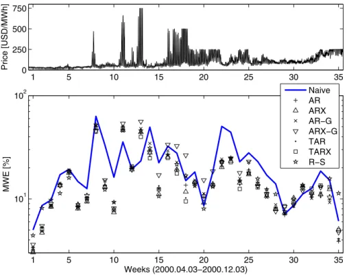
1 5 10 15 20 25 30 35 101 102 MWE [%] Weeks (2000.04.03−2000.12.03) 1 5 10 15 20 25 30 35 0 250 500 750 Price [USD/MWh ] Naive AR ARX AR−G ARX−G TAR TARX R−S
Figure 3: Hourly system prices (top panel; note the changing price cap 750 →500→250 USD/MWh) and Mean Weekly Errors for all forecasting methods (bottom panel; note the semi-log scale) during the whole test period: April 3 – December 3, 2000. Only ARX, ARX-G and TARX models use exogenous fundamental variables in the specification.
or roughly the same as TAR, the situation changed in favor of the latter in late 2000 when the minimum daily price increased above 70 USD/MWh. For the last seven weeks TAR outperformed TARX six times and gave the best overall forecast in terms of WRMSE three times. A similar effect could be observed for the AR and ARX models: while for the relatively calm period a ca. 10% decrease in MWE was observed with the additional fundamental variable, during the spiky weeks the improvement was negligible. It is not that surprising if we recall that at that time the situation in California was far from being normal, with the load-price relationship being substantially violated (see Fig. 1).
For the autoregressive models with GARCH noise this effect was even more striking. There was no clear winner among the two considered models, per-haps AR-G was even slightly better. In terms of MWE and WRMSE (see Tables 2-3) both models performed clearly not as good as the AR/ARX or
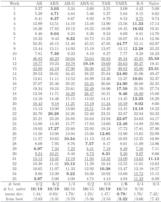
Table 2: Mean Weekly Errors (MWE) in percent for all weeks of the test period. Best results for each week are emphasized in bold. Results not passing the na¨ıve test are underlined. Measures of fit are summarized in the bottom rows. The first number (before the slash) indicates performance during the first 10 weeks and the second – during the latter 25 weeks.
Week AR ARX AR-G ARX-G TAR TARX R-S Na¨ıve 1 3.37 3.03 3.34 3.60 3.21 3.09 4.42 5.00 2 5.29 4.71 4.84 5.46 5.37 5.04 8.15 8.62 3 8.41 8.37 8.67 8.92 8.79 8.52 9.75 9.74 4 13.99 13.51 14.10 13.48 13.90 13.56 11.33 17.14 5 18.26 17.82 19.12 18.22 18.09 18.45 16.02 19.31 6 8.40 8.04 8.24 8.26 9.24 8.69 8.81 14.70 7 10.32 9.43 9.32 10.72 11.23 10.07 10.14 12.56 8 50.35 48.15 51.40 45.55 47.95 44.77 52.11 62.97 9 13.44 13.11 14.93 15.19 13.87 13.12 12.28 33.22 10 7.81 7.39 9.23 8.10 8.27 7.77 9.28 16.23 11 46.82 46.23 50.04 53.64 50.83 48.34 45.85 35.59 12 19.77 19.23 19.78 19.18 19.69 20.63 20.27 19.41 13 43.88 44.19 47.90 56.00 42.78 39.82 45.80 23.31 14 29.53 28.01 34.45 28.22 25.84 24.80 31.06 49.47 15 12.61 11.11 12.53 16.99 13.36 12.37 10.61 22.37 16 27.07 25.46 29.22 33.45 26.68 24.90 26.68 32.35 17 19.34 19.24 22.61 32.49 18.96 17.59 21.59 27.74 18 13.58 11.71 16.29 26.47 10.21 9.46 16.80 15.00 19 14.10 14.46 15.15 14.02 14.11 14.45 13.33 18.20 20 10.43 9.18 11.25 15.19 11.24 10.59 8.02 8.60 21 14.13 13.90 13.60 18.51 13.40 13.45 13.10 18.22 22 20.70 20.28 24.26 22.40 23.55 22.87 22.94 50.33 23 25.21 23.28 24.88 24.64 24.94 22.67 24.63 44.17 24 14.80 14.30 15.77 17.83 13.60 12.48 14.88 22.86 25 19.03 17.27 22.60 22.92 19.24 17.72 17.81 27.90 26 14.50 13.98 13.94 13.30 12.85 12.90 15.65 22.99 27 11.57 10.65 10.34 11.13 12.45 10.95 12.35 16.98 28 8.09 7.95 8.76 7.57 8.17 8.01 11.09 13.96 29 6.97 7.34 7.22 8.41 7.19 8.49 7.58 7.11 30 9.24 10.21 8.48 8.73 8.31 9.20 9.97 8.66 31 13.12 13.35 12.19 11.94 13.32 13.09 13.63 11.12 32 10.38 11.41 10.13 11.29 10.44 12.55 11.01 12.62 33 10.65 11.07 11.33 12.92 10.38 13.47 13.18 18.57 34 9.80 12.39 9.22 10.30 10.92 13.00 15.72 15.15 35 3.87 5.06 4.00 4.74 4.13 4.94 11.33 6.09 # best 0/2 5/2 1/3 0/2 0/3 1/6 3/4 0/3 # b.t. na¨ıve 10/19 10/19 10/18 10/15 10/19 10/18 9/16 – mean dev. 1.44/ 0.83/ 1.79/ 1.23/ 1.47/ 0.78/ 1.70/ 7.42/ from best /2.63 /2.31 /3.70 /5.56 /2.53 /2.22 /3.66 /7.42
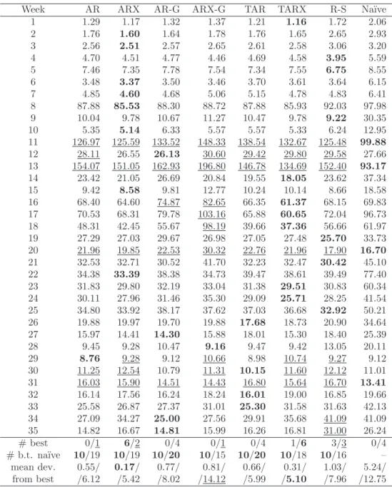
Table 3: Weekly Root Mean Square Errors (WRMSE) for all weeks of the test period. Best results for each week are emphasized in bold. Results not passing the na¨ıve test are underlined. Measures of fit are summarized in the bottom rows. The first number indicates performance during the first 10 weeks and the second – during the latter 25 weeks.
Week AR ARX AR-G ARX-G TAR TARX R-S Na¨ıve 1 1.29 1.17 1.32 1.37 1.21 1.16 1.72 2.06 2 1.76 1.60 1.64 1.78 1.76 1.65 2.65 2.93 3 2.56 2.51 2.57 2.65 2.61 2.58 3.06 3.20 4 4.70 4.51 4.77 4.46 4.69 4.58 3.95 5.59 5 7.46 7.35 7.78 7.54 7.34 7.55 6.75 8.55 6 3.48 3.37 3.50 3.46 3.70 3.61 3.64 6.15 7 4.85 4.60 4.68 5.06 5.15 4.78 4.83 6.41 8 87.88 85.53 88.30 88.72 87.88 85.93 92.03 97.98 9 10.04 9.78 10.67 11.27 10.47 9.78 9.22 30.35 10 5.35 5.14 6.33 5.57 5.57 5.33 6.24 12.95 11 126.97 125.59 133.52 148.33 138.54 132.67 125.48 99.88 12 28.11 26.55 26.13 30.60 29.42 29.80 29.58 27.66 13 154.07 151.05 162.93 196.80 146.78 134.69 152.40 93.17 14 23.42 21.05 26.69 20.84 19.55 18.05 23.62 37.34 15 9.42 8.58 9.81 12.77 10.24 10.14 8.66 18.58 16 68.40 64.60 74.87 82.65 66.35 61.37 68.15 69.83 17 70.53 68.31 79.78 103.16 65.88 60.65 72.04 96.73 18 48.31 42.45 55.67 98.19 39.66 37.36 56.66 61.97 19 27.29 27.03 29.67 26.98 27.05 27.48 25.70 33.73 20 21.96 19.85 22.53 30.32 22.76 21.96 17.90 16.70 21 32.53 32.71 30.52 41.70 32.23 32.47 30.42 45.10 22 34.38 33.39 38.38 34.73 39.47 38.61 39.49 77.40 23 31.83 29.80 32.19 33.04 31.38 29.51 30.83 60.34 24 30.11 27.96 31.46 35.30 29.09 25.71 28.25 41.54 25 34.80 33.92 38.17 37.62 37.03 36.68 32.92 50.21 26 19.88 19.97 19.70 19.88 17.68 18.73 20.90 34.64 27 15.97 14.41 14.30 15.88 18.01 15.30 18.40 25.39 28 9.45 9.28 10.47 9.16 9.47 9.42 13.05 20.11 29 8.76 9.28 9.12 10.66 8.98 10.74 9.27 9.12 30 11.25 12.54 10.79 11.31 10.15 11.60 12.12 11.01 31 16.03 15.90 14.51 14.43 16.80 15.64 16.70 13.41 32 16.14 17.56 16.24 18.24 16.01 19.00 16.85 19.66 33 25.58 26.87 27.37 31.01 25.30 31.58 31.63 42.13 34 27.09 34.27 25.00 27.56 29.91 35.68 41.09 41.09 35 14.82 16.67 14.81 15.99 16.26 16.81 31.00 26.24 # best 0/1 6/2 0/4 0/1 0/4 1/6 3/3 0/4 # b.t. na¨ıve 10/19 10/19 10/20 10/15 10/20 10/18 10/16 – mean dev. 0.55/ 0.17/ 0.77/ 0.81/ 0.66/ 0.31/ 1.03/ 5.24/ from best /6.12 /5.42 /8.02 /14.12 /5.99 /5.10 /7.96 /12.75
TAR/TARX models. In terms of MWE, AR-G yielded the best predictions for only four weeks (compared to two weeks for ARX-G) and was better than the na¨ıve method 30 times (compared to 25). Also in terms of WRMSE, the mean deviation from the best forecast was lower for the AR-G model in both periods. This is especially true for the volatile period, where the ARX-G model even failed to outperform the na¨ıve approach. Thus, we conclude that despite the heteroskedastic nature of the residuals in the autoregressive mod-els, the addition of a GARCH component in the specification does not improve the accuracy of point forecasts. ARX-G performed considerably worse than ARX while AR-G was still worse than AR, the simplest of all autoregressive models. These results somewhat contradict the reports of Garcia et al. (2005) who concluded that (seasonal) ARIMA-GARCH models outperformed simpler (seasonal) ARIMA models fitted to California (!) and Spanish data.
Finally, we found that also the non-linear R-S model failed to outperform the ARX and TARX approaches. Especially during the calm period observed MWE and WRMSE values were substantially higher than those of the other specified models. During the spiky weeks, when the price level increased dra-matically, the results for the R-S model were better. This was due to the fact that most hours were assigned to the spike regime, which by construction gave higher estimates for spot prices and volatility. But still, overall, the R-S model failed to provide better forecasts than the simple, linear AR model.
4.3
Interval forecasts
We further investigated the ability of the models to provide interval forecasts. While there is a variety of empirical studies on evaluating point forecasts in electricity markets (Szkuta et al., 1999, Nogales et al., 2002, Contreras et al., 2003, Rodriguez and Anders, 2004, Weron and Misiorek, 2005), to the best of our knowledge density or interval forecasts have not been investigated to date. However, such forecasts may be especially relevant for risk manage-ment purposes where one is more interested in predicting intervals for future price movements than simply point estimates. Therefore, this section provides additional results on interval forecasts for the out-of-sample period April 3 – December 3, 2000. In the following, only the results for the best model in each class in terms of point forecasts are described, i.e. the ARX model for the simple linear approach, the AR-G model for the models with an addi-tional GARCH component and the TARX specification as a representative of the threshold regime-switching models. However, the results for AR, ARX-G and TAR were similar to the better performing model in their class and are available upon request from the authors.
24 48 72 96 120 144 168 −20 −10 0 10 20 30 Hours (2000.04.03−09)
Deviation from MCP [USD/MWh
] ARX 24 48 72 96 120 144 168 −200 −100 0 100 Hours (2000.08.21−27)
Deviation from MCP [USD/MWh
] CI(50%) CI(90%) CI(99%) 24 48 72 96 120 144 168 −20 −10 0 10 20 30 Hours (2000.04.03−09)
Deviation from MCP [USD/MWh]
AR−G 24 48 72 96 120 144 168 −200 −100 0 100 Hours (2000.08.21−27)
Deviation from MCP [USD/MWh]
CI(50%) CI(90%) CI(99%)
Figure 4: Deviation of the day-ahead point forecasts and their respective 50%, 90% and 99% two-sided confidence intervals (CI) from the actual market clearing price (MCP) for two models: ARX (top panels) and AR-G (bottom panels), and for two weeks of the test period: the first week (April 3-9, 2000;left panels) and the 21stweek (August 21-27, 2000;
right panels).
For the AR/ARX, AR/ARX-G and TAR/TARX models interval forecasts were determined analytically (for details on calculation of conditional pre-diction error variance and interval forecasts we refer to Baillie and Boller-slev, 1992, BollerBoller-slev, 1986, Hamilton, 1994, Hansen, 1997, Ljung, 1999). How-ever, for the R-S model interval forecasts were determined via Monte Carlo simulations. For each hourn= 1000 simulations were run, based on estimated model parameters and probabilities for being in regimeRt ={1,2}. Then, us-ing the simulated forecasts for the spot price at timet+ 24 the corresponding confidence intervals were determined.
Afterwards, following Baillie and Bollerslev (1992) or Christoffersen and Diebold (2000), we evaluated the quality of the interval forecasts by comparing the nominal coverage of the models to the true coverage, see Figs. 4 and 5. Thus, for each of the models we calculated confidence intervals (CI) and
24 48 72 96 120 144 168 −20 −10 0 10 20 30 Hours (2000.04.03−09)
Deviation from MCP [USD/MWh
] TARX 24 48 72 96 120 144 168 −200 −100 0 100 Hours (2000.08.21−27)
Deviation from MCP [USD/MWh
] CI(50%) CI(90%) CI(99%) 24 48 72 96 120 144 168 −20 −10 0 10 20 30 Hours (2000.04.03−09)
Deviation from MCP [USD/MWh]
R−S 24 48 72 96 120 144 168 −200 −100 0 100 Hours (2000.08.21−27)
Deviation from MCP [USD/MWh]
CI(50%) CI(90%) CI(99%)
Figure 5: Deviation of the day-ahead point forecasts and their respective 50%, 90% and 99% two-sided confidence intervals (CI) from the actual market clearing price (MCP) for two models: TARX (top panels) and R-S (bottom panels), and for two weeks of the test period: the first week (April 3-9, 2000;left panels) and the 21stweek (August 21-27, 2000;
right panels).
determined the actual percentage of exceedances of the 50%, 90% and 99% two sided day-ahead CI of the models by the actual market clearing price (MCP). If the model implied interval forecasts were accurate then the percentage of exceedances should be approximately 50%, 10% and 1%, respectively. Note that for each week, 168 hourly values were determined and compared to the actual MCP.
Figures 4 and 5 show the deviations of the point forecasts and 50%, 90% and 99% two-sided CI from the market clearing price (MCP). Results for four models (ARX, AR-G, TARX and R-S) and for two weeks (April 3-9, 2000 and August 21-27, 2000) of the test period are displayed. Note that the width of the interval varies more for the TARX model than for its competitors, the R-S approach in particular. This is the case both for variations of interval lengths within certain hours or days and differences between calm and volatile periods.
Examining the deviations of the CI from the actual MCP for the first week of the test period (left panels in Figures 4-5), we find that for the ARX, AR-G and TARX models almost all confidence intervals include the actual MCP. This is especially true for the 90% and 99% intervals, but even for the 50% confidence level deviations from the actual MCP are rarely high enough to exclude the price from the interval. The results are different for the R-S model giving the narrowest CI estimates for the first week of the test period. For about one third of the time the actual MCP exceeds the 50% CI and approximately 5% of the prices lie outside the 90% CI. This is due to the fact that with high probability the calm period is assigned to the base regime, yielding rather narrow confidence intervals for the period.
Looking at the results for the 21st week of the test period (right panels in Figures 4-5), we find that due to the higher volatility in this period, the ARX and AR-G models give higher estimates for the (conditional) volatility while the R-S and TARX models give higher probabilities for staying in the spiky regime. Thus, CI forecasts for these models are much wider in comparison to the first week of the test period. For certain hours forecasted 99% CI are wider than 150 USD/MWh giving an extensive range of possible one-day ahead spot prices. As a result, only about 1.2% (7.1%) of the 99% (90%) CI for the TARX model fail to comprise the actual MCP. Results for the non-linear AR-G model are similar, yielding approximately 1.2% (13.1%) exceedances of the 99% (90%) CI. The ARX model performs significantly worse with approximately 3.6% (17.9%) exceedances of the 99% (90%) CI. Finally, the R-S model does not manage to outperform even the linear ARX model. The intervals are not wide enough to provide acceptable results: approximately 17.9% (36.3%) of the 99% (90%) CI fail to comprise the actual MCP.
Figure 6 displays the actual percentage of exceedances for the 35 weeks of the out-of-sample test period for the four models: ARX, AR-G, TARX and R-S. For the R-S model (lower right panel), obviously the number of exceedances is systematically too high due to the too narrow interval forecasts. The empirically observed number of exceedances is higher than the theoretical confidence level would suggest. This is true for all confidence levels of 50%, 90% and 99%. Most demonstrative, we observe that for a number of weeks more than 20% of the 99% CI are exceeded. This is also confirmed by the results in Table 4.
The results are substantially better for the ARX, AR-G and TARX models. We find that due to heavy tails in the residuals, for a confidence level of 99% the intervals are still too narrow. Yet, the TARX model is closest to being optimal. For the 99% level the average number of exceedances of the intervals is higher than it is expected theoretically, but is substantially lower than for
1 5 10 15 20 25 30 35 0 20 40 60 80 100 Weeks (2000.04.03−2000.12.03) ARX CI Exceedances [%] 1 5 10 15 20 25 30 35 0 20 40 60 80 100 Weeks (2000.04.03−2000.12.03) AR−G CI Exceedances [%] 1 5 10 15 20 25 30 35 0 20 40 60 80 100 Weeks (2000.04.03−2000.12.03) TARX CI Exceedances [%] CI(50%) CI(90%) CI(99%) 1 5 10 15 20 25 30 35 0 20 40 60 80 100 Weeks (2000.04.03−2000.12.03) R−S CI Exceedances [%]
Figure 6: Percent of exceedances of the 50%, 90% and 99% two-sided day-ahead confidence intervals (CI) by the actual market clearing price (MCP) for the ARX (top left), AR-G (top right), TARX (bottom left) and R-S (bottom right) models during all 35 weeks of the test period.
the R-S model. Regarding the 90% confidence levels, the ARX and AR-G models again underestimate the range of possible next-day prices leading to too narrow CI and too many CI exceedances (the AR-G model is slightly better though, despite its worse point forecasting performance). The TARX model, on the other hand, gives very good results for the interval forecasts of the 90% confidence level: the number of exceedances is approximately 11% during the calm and 9% during the spiky period. Finally, note that all three models overestimate the 50% CI. This, together with the underestimation of the upper quantiles (i.e. 90% and 99% CI), indicates that the distributions of the residuals have heavier tails than Gaussian. Apparently, neither the heteroskedastic component nor the regime-switching mechanism do a perfect job of modeling the heavy-tailed nature of the marginal distributions. Perhaps, time series models with heavy-tailed innovations should be utilized in this context (see e.g. Mugele et al., 2005, Nowicka-Zagrajek and Weron, 2002).
Table 4: Mean percent of exceedances of the 50%, 90% and 99% two-sided day-ahead confidence intervals (CI) by the actual market clearing price (MCP) for the ARX, AR-G, TARX and R-S models.
ARX AR-G Weeks 50% 90% 99% 50% 90% 99% 1-10 41.67 13.57 5.60 41.85 12.08 5.12 11-35 45.95 13.45 5.48 42.86 13.45 5.60 TARX R-S Weeks 50% 90% 99% 50% 90% 99% 1-10 37.32 11.31 4.58 61.01 26.79 12.08 11-35 38.19 8.86 3.17 65.74 29.52 14.00
In view of the very good performance of the TARX model both in point and interval predictions, the TARX model can be regarded as the overall winner. This contradicts the results of other studies by Dacco and Satchell (1999), Crawford and Fratantoni (2003) or Bessec and Bouabdallah (2005), where the forecasting performance of regime-switching models was reported to be rather poor.
The good results of the TARX and AR-G models in interval forecasting may also suggest the use of models with a combination of threshold autore-gression and heteroskedasticity like TAR(X)-GARCH models in future work. Such models have already been found to perform well for financial data. For instance, Chiang and Doong (2001) found that for daily stock returns the GARCH parameters of a TAR-GARCH(1,1) model were highly significant. Gospodinov (2005) used a TAR framework with GARCH errors to test for threshold nonlinearity in short-term interest rates and concluded that allowing for threshold nonlinearities in conditional mean and variance led to significant improvements of short-term forecasts.
5
Conclusions
In this paper we investigated the forecasting power of various time series mod-els for electricity spot prices. The modmod-els included different specifications of linear autoregressive time series with heteroskedastic noise and/or additional fundamental variables. Further, a non-linear, Markov regime-switching model with AR(1)-type processes as well as threshold regime-switching models (TAR and TARX) were considered. The models were tested on a time series of hourly
system prices and loads from the California power market. Data from the pe-riod July 5, 1999 – April 2, 2000 was used for calibration and from the pepe-riod April 3 – December 3, 2000 for out-of-sample testing.
Our findings support the adequacy of the tested models for point forecasts of electricity spot prices, also in comparison to earlier empirical studies. The best results were obtained using a non-linear TARX model and a relatively simple ARX model (in both cases the day-ahead load forecast was used as the exogenous/fundamental variable). The models with the additional GARCH component (AR/ARX-G), but also the R-S model, failed to outperform the rel-atively simple ARX approach. These findings show that an additional GARCH component does not help to improve results in point forecasting. Also R-S models are unable to provide better results than a simple linear approach.
For interval forecasting, following Baillie and Bollerslev (1992) or Christof-fersen and Diebold (2000) we evaluated the quality of the predictions by com-paring the nominal coverage of the models to the true coverage. We found that again the TARX model gave the best results. This time it was closely fol-lowed by the AR-G and ARX models. The non-linear Markov regime-switching model systematically underestimated the range of possible next-day electricity prices and yielded the worst results of all tested models.
We conclude that in contrast to other studies on the failure of non-linear models in forecasting (Dacco and Satchell, 1999, Crawford and Fratantoni, 2003, Bessec and Bouabdallah, 2005), in our case the TARX model gave the best overall results. Both for point and interval forecasting the model outper-formed most of its competitors and was the best in several of the considered criteria. Consequently, we recommend the threshold AR/ARX models for forecasting of highly volatile electricity spot prices, especially for purposes of determining risk figures based on confidence intervals.
References
Baillie, R. and T. Bollerslev (1992). “Prediction in dynamic models with time-dependent conditional variances”,Journal of Econometrics 52, 91-113. Bessec, M., and O. Bouabdallah (2005). “What causes the forecasting failure of
Markov-switching models? A Monte Carlo study”, Studies in Nonlinear Dynamics and Econometrics 9(2), Article 6.
Bierbrauer, M., S. Tr¨uck, and R. Weron (2004). “Modeling electricity prices with regime switching models”,Lecture Notes on Computer Science 3039, 859-867.