Selfish Distributed Compression over Networks
Aditya Ramamoorthy
∗, Vwani Roychowdhury
†, Sudhir Kumar Singh
†∗ Department of Electrical and Computer Engineering, Iowa State University, Ames, Iowa 50011. Email: [email protected]
†Department of Electrical Engineering, University of California, Los Angeles, CA 90095. Emails:{vwani,suds}@ee.ucla.edu
Abstract—We consider the min-cost multicast problem (under network coding) with multiple correlated sources where each terminal wants to losslessly reconstruct all the sources. This can be considered as the network generalization of the classical distributed source coding (Slepian-Wolf) problem. We study the inefficiency brought forth by the selfish behavior of the terminals in this scenario by modeling it as a noncooperative game among the terminals. The solution concept that we adopt for this game is the popular local Nash equilibrium (Waldrop equilibrium) adapted for the scenario with multiple sources. The degradation in performance due to the lack of regulation is measured by the
Price of Anarchy (POA), which is defined as the ratio between the
cost of the worst possible Waldrop equilibrium and the socially optimum cost. Our main result is that in contrast with the case of independent sources, the presence of source correlations can significantly increase the price of anarchy. Towards establishing this result we make several contributions. We characterize the socially optimal flow and rate allocation in terms of four intuitive conditions. This result is a key technical contribution of this paper and is of independent interest as well. Next, we show that the Waldrop equilibrium is a socially optimal solution for a different set of (related) cost functions. Using this, we construct explicit examples that demonstrate that the POA>1and determine near-tight upper bounds on the POA as well. The main techniques in our analysis are Lagrangian duality theory and the usage of the supermodularity of conditional entropy. Finally, all the techniques and results in this paper will naturally extend to a large class of network information flow problems where the Slepian-Wolf polytope is replaced by any contra-polymatroid (or more generally polymatroid-like set), leading to a nice class of succinct multi-player games and allow the investigation of other practical and meaningful scenarios beyond network coding as well.
I. INTRODUCTION
In large scale networks such as the Internet, the agents in-volved in producing and transmitting information often exhibit selfish behavior e.g. if a packet needs to traverse the network of various ISP’s, each ISP will behave in a greedy manner and ensure that the packet spends the minimum time on its network. While this minimizes the ISP’s cost it may not be the best strategy from a overall network cost perspective. Selfish routing, that deals with the question of network performance under a lack of regulation has been studied extensively (see [15], [20]) and has developed as an area of intense research activity. However, by and large most of these studies have considered the network traffic injected into the network at various sources to be independent.
From an information theoretic perspective there is no need to consider the sources involved in the transmission to be
independent. In this paper we initiate the study of network optimization issues related to the transmission of correlated sources over a network when the agents involved are selfish. In particular, we concentrate on the problem of multicasting correlated sources over a network to different terminals, where each terminal is interested in losslessly reconstructing all the sources. We assume that the network is capable of network coding. Under this scenario, a generalization of the classical Slepian-Wolf theorem of distributed source coding [8] holds for arbitrary networks. In particular when the network per-forms random linear network coding each terminal can recover the sources under appropriate conditions on the Slepian-Wolf region and the capacity region of the terminals with respect to the sources, thereby allowing distributed source coding over networks. The selfish agents in our set-up are the terminals who pay for the resources. Each terminal aims to minimize her own cost while ensuring that she can satisfy her demands. It is important to note that this is a generalization of the problem of minimum cost selfish multicast of independent sources considered by Bhadra et al. [3].
Our Results:
In this work, we model the scenario as a noncooperative game amongst the selfish terminals who request rates from sources and flows over network paths such that their individual cost is minimized (i.e. with no regard for social welfare) while allowing for reconstruction of all the sources. We investigate properties of the socially optimal solution and define appropriate solution concepts (Nash equi-librium and Waldrop equiequi-librium) for this game and investigate properties of the flow-rates at equilibrium. We briefly describe our contributions below.i) Characterization of social-optimality conditions. The prob-lem of computing the socially optimal cost is a convex pro-gram. We present a precise characterization of the optimality conditions of this convex program in terms of four intuitive conditions, using Lagrangian duality theory and by judiciously exploiting the super-modularity of conditional entropy. ii) Demonstrating the equivalence of flow-rates at equilibrium
with social-optimal solutions for alternative instances. We
consider certain meaningful market models that split resource costs amongst the different terminals and show that the flows and rates under the game-theoretic equilibriums are in fact socially optimal solutions for a different set of cost functions. This characterization allows us to quantify the degradation caused by the lack of regulation. The measure of performance degradation due to such loss in regulation that we adopt is
the Price of Anarchy (POA), which is defined as the ratio between the cost of the worst possible equilibrium and the socially optimum cost [9], [17], [21], [20].
iii) Showing that source correlation induces anarchy. The main result of this paper is that the presence of source correlations can significantly increase the POA under reasonable cost-splitting mechanisms. This is in stark contrast to the case of multicast with independent sources, where for a large class of cost functions, cost-splitting mechanisms can be designed that ensure that the price of anarchy is one. We construct explicit examples where the POA is greater than one and also obtain an upper bound on the POA which is near tight.
Finally, we expect that the techniques developed in this paper will be applicable to a large class of network information flow problems with correlated sources where the Slepian-Wolf polytope is replaced by polymatroid-like objects. These include multi-terminal source coding with high resolution [23] and the CEO problem [18].
Background and Related Work:
Distributed source coding (or distributed compression) (see [5], Ch. 14 for an overview) considers the problem of compressing multiple discrete memoryless sources that are observing correlated ran-dom variables. The landmark result of Slepian and Wolf [22] characterizes the feasible rate region for the recovery of the sources. However, the problem of Slepian and Wolf considers a direct link between the sources and the terminal. More generally one would expect that the sources communicate with the terminal over a network. Different aspects of the Slepian-Wolf problem over networks have been considered in ([2], [6], [19]). Network coding (first introduced in the seminal work of Ahlswede et al. [1]) for correlated sources was considered by Ho et al. [8]. They considered a network with a set of sources and a set of terminals and showed that as long as the minimum cuts between all non-empty subsets of sources and a particular terminal were sufficiently large (essentially as long as the Slepian-Wolf region of the sources has an intersection with the capacity region of a given terminal), random linear network coding over the network followed by appropriate decoding at the terminals achieves the Slepian-Wolf bounds.The problem of minimum cost multicast under network coding has been addressed in the work of [13], [12]. The multicast problem has also been examined by considering selfish agents [3], [10], [11]. Our work is closest in spirit to the analysis of Bhadra et al. [3] that considers selfish terminals. In this scenario, for a large class of edge cost functions, they develop a pricing mechanism for allocating the edge costs among the different terminals and show that it leads to a globally optimal solution to the original optimization problem, i.e. the price of anarchy is one. Their POA analysis is similar to that in the case of selfish routing [21], [20]. Our model is more general and our results do not generalize from theirs in a straightforward manner. In particular, we need to judiciously exploit several non-trivial properties of the Slepian-Wolf polytope in our analysis.
II. THEMODEL
Consider a directed graph G = (SU T U V, E). There is a set of source nodes S that may be correlated and a set of sinksT that are the terminals (i.e. receivers). Each source node observes a discrete memoryless sourceXi. The Slepian-Wolf
region of the sources is assumed to be known and is denoted RSW. For notational simplicity, let NS = |S|, NT = |T|,
S = {1,2, . . . , NS}, and T = {t1, t2, . . . , tNT}. The set
of paths from source s to terminal t is denoted by Ps,t.
Further, define Pt = ∪s∈SPs,t i.e. the set of all possible
paths going to terminal t, and P = ∪t∈TPt, the set of all
possible paths. A flow is an assignment of non-negative reals to each path P ∈ P. The flow on P is denoted fP. A rate
is a function R : S×T −→ R+, i.e. the rate requested by
the terminalt from the source s is Rs,t. We will refer to a
flow and rate pair(f, R)as flow-rate. Also, let us denote the rate vector for terminalt by Rt and the vector of requested
rates at sourcesbyρs i.e.Rt= (R1,t, R2,t, . . . , RNS,t)and
ρs= (Rs,t1, Rs,t2, . . . , Rs,tNT).
Associated with each edgee∈E is a costce, which takes
as argument a scalar variablezethat depends on the flows to
various terminals passing through e. Similarly, let ds be the
cost function corresponding to the source s, which takes as argument a scalar variable ys that depends on the rates that
various terminals request from s. These functions ce’s and
ds’s are assumed to be convex, positive, differentiable and
monotonically increasing. Further, the functions R ce(x)
x dx
are also convex, positive, differentiable and monotonically increasing. In particular, these conditions are satisfied by functions likexa, a >1andxebx, b >0 among others.
The network connection we are interested in supporting is one where each terminal can reconstruct all the sources. i.e. we need to jointly allocate rates and flows for each terminal so that it can reconstruct the sources. We now present a formal description of the optimization problem under consideration.
Min-Cost Multicast with Multiple Sources:
Let us call the quadruple(G, c, d,RSW)an instance. The problem of minimizing the total cost for the instance (G, c, d,RSW) can be formulated as minimize C(f, R) =X e∈E ce(ze) + X s∈S ds(ys) subject to fP ≥0 ∀P ∈P (N IF −CP) X P∈Ps,t fP ≥Rs,t ∀s∈S,∀t∈T (1) Rt∈RSW ∀t∈Twhere ze,∀e ∈ E is a function of xe,t1, xe,t2, . . . , xe,tNT, that we shall denote ze(xe,t1, xe,t2, . . . , xe,tNT) with xe,t = P
P∈Pt:e∈PfP ∀e ∈ E, ∀t ∈ T, and ys,∀s ∈ S is a
function ofρsthat we will denoteys(ρs).
The formulation above is similar to the one presented in [3]. However since we consider source correlations as well, their formulation is a specific case of our formulation. Since network coding allows the sharing of edges, the penalty at
an edge is only the maximum and not the sum i.e. ze is
the maximum flow (among the different terminals) across the edge e. Similarly, the penalty at the sources for higher resolution quantization is also driven by the maximum level requested by each terminal i.e. ys is also maximum. In this
work, for differentiability requirements the maximum function will be approximated asLp norm withp→ ∞. Nevertheless,
most of our analysis is done where ze and ys are
non-decreasing functions partially differentiable with respect to their arguments, such that ce(ze) and ds(ys) are convex,
positive, differentiable and monotonically increasing. Note that in the formulation above, the objective function is convex and all constraints are linear which implies that this is a convex optimization problem.
The constraint (1) above models the fact that the total flow from the source s to a terminal t needs to be at least Rs,t.
Finally, the rate point of each terminalRtneeds to be within
the Slepian-Wolf polytope. A flow-rate (f, R) satisfying all the conditions in the above optimization problem (i.e.
(NIF-CP) ) will be called a feasible flow-rate for the instance
(G, c, d,RSW) and the cost C(f, R) will be referred to as
social cost corresponding to this flow-rate. Also, we will call
a solution(f∗, R∗)of the above problem as an OPT flow-rate for the instance (G, c, d,RSW).
Consider a feasible flow-rate (f, R) for the above optimization problem. It can be seen that the value of the flow from A ⊆ S to a terminal t ∈ T is P
P∈∪s∈APs,tfP ≥
P
s∈ARs,t. Since Rt ∈ RSW the result of [8] shows that random linear network coding followed by appropriate decoding at the terminals can recover the sources with high probability. Conversely the result of [2] shows the necessity of the existence of such a flow.
Terminals’ Incentives and the Distributed
Com-pression Game:
The above formulation for social cost minimization for the instance (G, c, d,RSW) disregards the fact that the agents who pay for the costs incurred at the edges and the sources may not be cooperative and may have incentives for strategic manipulation. In this work we consider the scenario where the terminals pay for the network resources they are being provided. The terminals are noncooperative and will behave selfishly trying to minimize their own respective costs without regard to the social cost, while ensuring that they can reconstruct all the sources. We have the following assumptions.(i) Let (f, R) denote a feasible flow rate for the instance (G, c, d,RSW). The network operates via random linear net-work coding over the subgraph of G induced by the cor-responding {ze} for e ∈ E. The terminals are capable of
performing appropriate decoding to recover the sources. (ii)Each terminal t ∈ T can request for any specific set of flows on the paths P ∈ Pt and rates Rt as long as such a
request allows reconstruction of the sources at t. There is a mechanism in the network by means of which this request is accommodated i.e. the subgraph over which random linear network coding is performed is adjusted appropriately.
In this work we wish to characterize flow-rates that represent an equilibrium among selfish terminals while they act strate-gically to minimize their own costs. Furthermore, we shall systematically study the loss that occurs due to the mismatch between the social goals and terminal’s selfish goals.
Towards this end, we now formally model the game orig-inating from the selfish behavior of the terminals. We model this game as a normal formal game[16], i.e. a static one shot strategic game of complete information, which we refer to as
Distributed Compression Game(DCG).
A normal form game, denoted (N,{Ai}i∈N,{i}i∈N),
consists of the set of playersN, the tuple of set of strategiesAi
for each playeri∈N, and the tuple of preference relationsi
for each playeri∈Non the setA=×i∈NAi. Fora, b∈A,
ai b means that the player i prefers the tuple of strategies
a to the tuple of strategies b. In the context of Distributed
Compression Game, given an instance (G, c, d,RSW), these parameters are defined as follows.
1) The Distributed Compression Game:
Players: N = T, i.e. the terminals are the players. This is because, as mentioned above, the terminals are the users and they are the ones who pay for the network resources they are being provided.
Strategies: The strategy set of a player t ∈ T consists of tuples(ft,Rt)where
• ftis the vector of flows on paths going tot, i.e. the vector
of values fP for all P ∈Pt, and recall that Rt denotes
the rate vector for terminalt;
• fP ≥ 0 ∀P ∈ Pt,PP∈Ps,tfP ≥ Rs,t ∀s ∈ S and Rt∈RSW. Therefore, At= (ft,Rt) : fP ≥0 ∀P ∈Pt, P P∈Ps,tfP ≥Rs,t ∀s∈S, Rt∈RSW . (2)
Note that a feasible flow-rate (f, R) for the instance (G, c, d,RSW)is an element of the setA=×t∈TAt defined
for the same instance.
Preference Relations: To specify the preference relation of terminal t ∈ T, we need to know how much does she pay given a feasible flow-rate(f, R)i.e. what fractions of the costs at various edges and sources are being paid byt? To this end, we need market models, i.e. mechanisms for splitting the costs among various terminals.
Edge Costs: At a flowf, the cost of an edgee∈Eisce(ze).
It is split among the terminalst∈T, each paying a fraction of this cost. Let us say that the fraction paid by the player t is Ψe,t(xe) i.e. the player t pays ce(ze)Ψe,t(xe) for the
edgeewherexe denotes the vector(xe,t1, xe,t2, . . . , xe,tNT). Of course, P
t∈TΨe,t(xe) = 1 to ensure that the total cost
is borne by someone or the other. The total cost borne by t across all the edges isP
e∈Ece(ze)Ψe,t(xe), denotedCE(t)(f).
Source Costs: At a rateR, the cost for the sourcesisds(ys),
which is split among the terminals t ∈ T, such that t pays a fraction Φs,t(ρs) i.e. the player t paysds(ys)Φs,t(ρs) for
the source s. Of course,P
t∈TΦs,t(ρs) = 1. Therefore, the
total cost borne by t for all sources, denoted CS(t)(R), is P
s∈Sds(ys)Φs,t(ρs).
Thus, with the edge-cost-splitting mechanism Ψ and the
source-cost-splitting mechanism Φ, the total cost incurred by the playert∈T at flow-rate(f, R)denotedC(t)(f, R)is
C(t)(f, R) = CE(t)(f) +CS(t)(R) = X e∈E ce(ze)Ψe,t(xe) + X s∈S ds(ys)Φs,t(ρs).
Now, each terminal t would like to minimize its own cost i.e. the function C(t)(f, R) and therefore the pref-erence relations {t} are as follows. For two flow-rates
(f, R) ∈ A and ( ˜f ,R˜) ∈ A, (f, R) t ( ˜f ,R˜) if and
only if C(t)(f, R) ≤ C(t)( ˜f ,R˜). Also, (f, R) ≻t ( ˜f ,R˜) iff
C(t)(f, R)< C(t)( ˜f ,R˜).
We will call (G, c, d,RSW,Ψ,Φ) as an instance of the Distributed Compression Game.
2) Solution Concepts for the Distributed Compression Game: We now outline the possible solution concepts in
our scenario. These are essentially dictated by the level of sophistication of the terminals. Sophistication refers to the amount of information and computational resources available to a terminal. In this work we shall work with two different solution concepts that we now discuss.
a) Nash Equilibrium. The solution concept of Nash equlib-rium requires the complete information setting and requires each terminal to compute her best response to any given tuple of strategies of the other players. For notational simplicity, let f−t be the vector of flows on paths not going to terminal t
i.e. the vector of values fP for all P ∈ P−Pt, therefore
f = (f−t, ft). Similarly, R−t is the vector of rates
corre-sponding to all players other thant, thereforeR= (R−t,Rt).
In our setting, the best response problem of a terminal t is to minimize her cost function C(t)(f
−t, ft,R−t,Rt) over
(ft,Rt)∈At given any(f−t,R−t). Therefore a Nash
flow-rate is defined as follows.
Definition 1: (Nash flow-rate) A flow-rate (f, R) feasible for the instance(G, c, d,RSW)is at Nash equilibrium, or is a Nash flow-rate for instance (G, c, d,RSW,Ψ,Φ), if ∀t∈T,
C(t)(f, R)≤C(t)(f−t,f˜t,R−t,R˜t) ∀( ˜ft,R˜t)∈At.
We note that computing the best response will in general require a given terminal to know flow assignments on all possi-ble paths and rate vectors for all the terminals. Moreover, con-vexity of the objective function inN IF−CP (i.e. social cost C(f, R)) does not imply convexity of C(t)(f−t, ft,R−t,Rt)
in the variables (ft,Rt) ∈ At in general. Therefore the
computational requirements at the terminals may be large. Consequently Nash equilibrium does not seem to be an appro-priate solution concept for the Distributed Compression Game when we look through the algorithmic lens.
b) Waldrop Equilibrium. From a practical standpoint, a terminal may only have partial knowledge of the system and may be computationally constrained. A solution concept
more appropriate under such situations is that of local Nash equilibrium or Waldrop equilibrium that is widely adopted in selfish routing and transportation literature[20], [14], [7]. We note that this solution concept has also been utilized in [3]. We first present the precise definition of the Waldrop equilibrium in our case and then provide an intuitive justification. Towards this end, we need to define the marginal cost of a path.
Definition 2: (Marginal Cost of a Path) For aP ∈Ptits
marginal cost is CP(f) :=Pe∈P
ce(ze)Ψe,t(xe)
xe,t .
Therefore, for the terminalt, the total cost for the edges,CE(t), can be equivalently written asCE(t)(f) =P
P∈PtCP(f)fP.
Definition 3: (Waldrop flow-rate) A flow-rate(f, R) feasi-ble for the instance(G, c, d,RSW)is at local Nash equilibrium, or is a Waldrop flow-rate for instance(G, c, d,RSW,Ψ,Φ), if it satisfies the following conditions.
(1)∀t∈T, ∀s∈S, we haveP P∈Ps,tfP =Rs,t. (2)∀t∈T, we have P s∈SRs,t=H(XS). (3) ∀t ∈ T, ∀s ∈ S, P, Q ∈ Ps,t with fP > 0, CP(f) ≤ CQ(f).
(4) For t ∈ T, let j ∈ S participates in all tight rate inequalities involving i ∈ S (i.e. if A ⊆ S, such that i ∈ A and P
l∈ARl,t = H(XA|X−A)1, then j ∈ A) and
letP ∈Pi,t, Q∈Pj,t withfP >0then we have
CP(f) + ∂CS(t)(R) ∂Ri,t ≤CQ(f) + ∂CS(t)(R) ∂Rj,t .
Intuitively, conditions (1) and (2) require that each terminal re-quests as little rate and flow as possible. Condition (3) ensures that an infitesimally small change in flow allocations from path P (wherefP >0) to pathQwhereP, Q∈Ps,t, will increase
the sum cost along paths inPt. Now, consider an infitesimally
small change in flow allocation fromP ∈Pi,t(wherefP >0)
toQ∈Pj,t. This also requires a corresponding change in the
rates requested from sources i and j by terminal t. Under certain constraints on the sourcej, Condition (4) ensures that the overall effect of this change will serve to increase terminal t’s cost. The conditions on the sourcej are well-motivated in light of the characterization of Nash flow-rate at the end of section III in the case when the best response problem of every terminal is convex.
We remark that a Nash flow-rate may not always be a Wal-drop flow-rate and vice versa. When sources are independent, condition (2) implies that Rs,t=H(Xs)for alls∈S, t∈T
and it is not required to check the condition (4). Also we can recover condition (3) by setting i=j in condition (4). They are stated separately for the sake of clarity.
As we discussed earlier, the solution concept based on Waldrop equilibrium seems more suitable to our scenario and consequently we define the price of anarchy [9], [17], [20] in terms of Waldrop flow-rate instead of Nash flow-rate.
Definition 4: Price of Anarchy(POA): LetCbe a class of edge cost functions,Dbe a class of source cost functions, G be a class of networks/graphs, Ψ be an edge cost splitting
1We useH(X
A|X−A)andH(XA|XAc)interchangeably in the text to denote the joint entropy of the sources in setAgiven the remaining sources.
mechanism, Φ be a source cost splitting mechanism, and M be a set of Slepian-Wolf polytopes. We will refer to (G,C,D,Ψ,Φ,M) as a scenario. The price of anarchy for the scenario(G,C,D,Ψ,Φ,M), denotedρ(G,C,D,Ψ,Φ,M), is defined as ρ(G,C,D,Ψ,Φ,M) = max G∈G,c∈C,d∈D,RSW∈M 1 COP T(G, c, d,RSW) max
(f, R)is a Waldrop flow-rate for(G, c, d,RSW,Ψ,Φ)
C(f, R)
,
where COP T(G, c, d,RSW) refers to the optimal cost of
N IF−CP for the instance(G, c, d,RSW). Let us denote the set of Slepian-Wolf polytopes corresponding to the case where there are no source correlations (i.e. H(XA|X−A) =H(XA)
for allA∈S) byMind(subscriptinddenotes - independent) and the set of Slepian-Wolf polytopes corresponding to the case where sources are correlated (i.e. there existsA⊆S with H(XA|X−A)< H(XA)) byMc. Also, we useGall to denote
the class of all graphs where everyt∈Tis connected to every s∈S, andGdsw(subscriptdsw denotes - direct Slepian-Wolf)
to denote the class of complete bipartite graphs between the set of sources and the set of terminals. Note thatGdswcorresponds
to the case where every terminals is directly connected to every source by an edge and no network coding is required. A question we will be most concerned with in this paper is whether ρ(G,C,D,Ψ,Φ,Mc) > ρ(G,C,D,Ψ,Φ,Mind),
and in particular whether ρ(G,C,D,Ψ,Φ,Mc) > 1 but
ρ(G,C,D,Ψ,Φ,Mind) = 1 for meaningful classes of cost
functions C,D and reasonable splitting mechanisms Ψ and Φi.e. does correlation induce anarchy?
III. CHARACTERIZING THEOPTIMALFLOWS ANDRATES In this section, we investigate the properties of an OPT flow-rate via Lagrangian duality theory [4]. Since the optimization problem (NIF-CP) is convex and the constraints are such that the strong duality holds, the Karush-Kuhn-Tucker(KKT) conditions exactly characterize optimality [4]. Therefore, we start out by writing the Lagrangian dual of NIF-CP,
L=X e∈E ce(ze) + X s∈S ds(ys)− X P∈P µPfP +X s∈S X t∈T λs,t(Rs,t− X P∈Ps,t fP) +X t∈T X A⊆S νA,t H(XA|XAc)− X i∈A Ri,t !
whereµP ≥0, λs,t≥0andνA,t≥0are the dual variables
(i.e. Lagrange multipliers). For notational simplicity, let us denote the partial derivative of ze with respect to xe,t, ∂xe,t∂ze
byze,t′ . Note that the partial derivative ofxe,tw.r.t. tofP is1
for aP ∈Pt. Similarly, we denote the partial derivative ofys
with respect to Rs,t, ∂Rs,t∂ys by y
′
s,t. The KKT conditions are
then given by the following equations that hold∀s∈S, t∈T, ∂L ∂fP =X e∈P c′e(ze)z ′ e,t(xe)−µP−λs,t= 0∀P ∈Ps,t, (3) ∂L ∂Rs,t =d′s(ys)y ′ s,t(ρs) +λs,t− X A⊆S:s∈A νA,t= 0 (4)
along with the feasibility of the flow-rate (f, R) and the complementary slackness conditionsµPfP = 0for allP ∈P,
λs,t(Rs,t −PP∈Ps,tfP) = 0 for all s ∈ S, t ∈ T, and
νA,t H(XA|XAc)−P i∈ARi,t
= 0for allA⊆S, t∈T. Let us now interpret the KKT conditions at the OPT
flow-rate(f∗, R∗). Suppose thatfP∗ >0forP ∈Ps,t. Then due to
complementary slackness, we haveµ∗P = 0 and consequently from equation (3) we get P
e∈Pc
′
e(ze∗)z
′
e,t(x∗e) = λ∗s,t i.e.
if there exists another path Q ∈ Ps,t such that fQ∗ > 0
then P e∈Pc ′ e(ze∗)z ′ e,t(x∗e) = P e∈Qc ′ e(ze∗)z ′ e,t(x∗e). On
fur-ther investigation we can obtain four necessary and sufficient conditions for optimality. Due to lack of space we will omit the proof of the necessity of these four conditions under strict convexity of the various cost functions and instead concentrate on the proof of sufficiency of these conditions for optimality.
Theorem 5: A feasible flow-rate (f, R) for the instance (G, c, d,RSW), which satisfies the following four conditions is an OPT flow-rate for the instance(G, c, d,RSW). Also, there is always an OPT flow-rate that satisfies these four conditions. Further, when the edge cost functionscefor alle∈Eand the
source cost functionsdsfor alls∈S are strictly convex, that
is when the optimization problem (NIF-CP) is strictly convex, these conditions are also necessary for optimality.
1) ∀t∈T, ∀s∈S, we haveP P∈Ps,tfP =Rs,t. 2) ∀t∈T, we have P s∈SRs,t=H(XS). 3) ∀t ∈ T, ∀s ∈ S, P, Q ∈ Ps,t with fP > 0, P e∈Pc ′ e(ze)z ′ e,t(xe)≤Pe∈Qc ′ e(ze)z ′ e,t(xe).
4) Fort∈T, suppose that there existi, j ∈S that satisfy the following property. If A⊆S, such that i∈A and P
l∈ARl,t=H(XA|X−A), thenj∈A. For suchiand
j letP ∈Pi,t, Q∈Pj,t withfP >0. Then
X e∈P c′e(ze)z ′ e,t(xe) +d ′ i(yi)y ′ i,t(ρi) ≤X e∈Q c′e(ze)z ′ e,t(xe) +d ′ j(yj)y ′ j,t(ρj).
Proof: We prove that the above four conditions imply
optimality of(f, R). Our assumptions guarantee that the opti-mization problem (NIF-CP) for the instance(G, c, d,RSW)is convex and since all the feasibility constraints are linear, strong duality holds [4]. This implies that the KKT conditions are necessary and sufficient for optimality. We show that a feasible flow-rate (f, R) with the above four properties satisfies the KKT conditions for the instance(G, c, d,RSW)for a suitable choice of the dual variables given below.
Choosing λi,t’s: λi,t := minP∈Pi,t
P e∈Pc ′ e(ze)z ′ e,t(xe).
a Pi ∈ Pi,t such that fPi > 0 then we have λi,t = P e∈Pic ′ e(ze)z ′ e,t(xe).
Choosing µP’s: For P ∈ Pi,t take µP :=
P e∈Pc ′ e(ze)z ′ e,t(xe)−λi,t.
ChoosingνA,t’s: Lethi,t:=d
′
i(yi)y
′
i,t(ρi)+λi,t. Letπdenote
a permutation such that 0≤hπ(1),t≤hπ(2),t ≤. . . hπ(NS),t.
Now take νA,t= hπ(1),t ifA={π(1), π(2), . . . , π(NS)} hπ(i),t−hπ(i−1),t if A={π(i), . . . , π(NS)} and2≤i≤NS 0 otherwise.
Now, with the above choice of dual variables we will check all the KKT conditions one by one.
Dual Feasibility:
• λi,t ≥ 0 as ce and ze are non-decreasing functions i.e.
c′e(ze)≥0 andz
′
e,t(xe)≥0.
• µP ≥ 0 by the definition because λi,t ≤
P e∈Pc ′ e(ze)z ′ e,t(xe)∀P ∈Pi,t. • νA,t≥0 by definition.
KKT Conditions as per equation 3: ∂L ∂fP =X e∈P c′e(ze)z ′ e,t(xe)−λi,t−µP =X e∈P c′e(ze)z ′ e,t(xe)−λi,t− X e∈P c′e(ze)z ′ e,t(xe)−λi,t ! = 0
KKT Conditions as per equation 4: ∂L ∂Rπ(i),t =d′π(i)(yπ(i))y ′ π(i),t(ρπ(i)) +λπ(i),t− X A⊆S:π(i)∈A νA,t =hπ(i),t− X A⊆S:π(i)∈A νA,t =hπ(i),t− X j∈{1,2,...,i} ν{π(j),π(j+1),...,π(NS)},t =hπ(i),t−[hπ(1),t+ (hπ(2),t−hπ(1),t) + (hπ(3),t−hπ(2),t) +· · ·+ (hπ(i),t−hπ(i−1),t)] =hπ(i),t−hπ(i),t= 0.
Complementary Slackness Conditions:
• µPfP = 0 for all P ∈ P. Let P ∈ Pi,t and
fP > 0 then using Condition 3 and definition of λi,t
we get P
e∈Pc
′
e(ze)z
′
e,t(xe) = λi,t and therefore, µP =
P e∈Pc ′ e(ze)z ′ e,t(xe)−λi,t = 0.
• λs,t(Rs,t−PP∈Ps,tfP) = 0 for all s ∈ S, t ∈ T. This
follows from the Condition1.
• νA,t H(XA|XAc)−P
i∈ARi,t= 0for all A⊆S, t∈T.
Note that νA,t = 0 except for A = {π(i), π(i +
1), . . . , π(NS)}, fori = 1,2, . . . , NS. Therefore the only
condition that needs to be checked is that if PNS
j=iRπ(j),t>
H(Xπ(i), Xπ(i+1), . . . , Xπ(NS)|Xπ(i−1), . . . , Xπ(1)), then
hπ(i),t−hπ(i−1),t= 0.
Towards this end let j ∈ {π(i), π(i+ 1), . . . , π(NS)}, and
let Aj be the minimum cardinality set such that j ∈Aj and
P l∈AjRl,t=H(XAj|X−Aj)i.e. Aj= arg min A⊆S:j∈A,P l∈ARl,t=H(XA|X−A) |A|.
Such a set Aj always exists because from Condition 2 we
have PNS
l=1Rl,t = H(X1, . . . , XNS) and therefore the set
A⊆S:j∈A,P
l∈ARl,t=H(XA|X−A) is not empty.
We claim that there exists a j∗ ∈ {π(i), π(i +
1), . . . , π(NS)} such that Aj∗ ∩ {π(1), π(2), . . . , π(i−1)} is not empty. If this is not true then clearly we have ∪πj=(NSπ(i))Aj = {π(i), π(i + 1), . . . , π(NS)} and
using the supermodularity property of conditional entropy (ref. Lemma 10), we obtain Pπ(NS)
j=π(i)Rj,t =
H(Xπ(i), Xπ(i+1), . . . , Xπ(NS)|Xπ(i−1), . . . , Xπ(1))
which is a contradiction, therefore we must have such a j∗ ∈ {π(i), π(i + 1), . . . , π(NS)} such that
Aj∗∩ {π(1), π(2), . . . , π(i−1)} is not empty.
Next, we show that there exists a source k ∈ {π(1), π(2), . . . , π(i − 1)} such that if j∗ ∈ A and P
l∈ARl,t = H(XA|X−A), then k ∈ A. Towards this
end suppose that there exist subsets S1 and S2 of such
that j∗ ∈ S
1 ∩S2 and Pl∈S1Rl,t = H(XS1|X−S1) and P
l∈S2Rl,t = H(XS2|X−S2), then using the supermodular-ity property of conditional entropy we can show that rate inequality involvingS1∩S2 is also tight ( Lemma 10) i.e.
P
l∈S1∩S2Rl,t = H(XS1∩S2|X−(S1∩S2)). This implies that Aj∗, being of minimum cardinality, is the intersection of all sets that havej∗ as a member on which the rate inequality is tight i.e. Aj∗ = \ A⊆S {A:j∗∈A,X l∈A Rl,t=H(XA|X−A)}.
Moreover note that Aj∗ is not a singleton set since Aj∗ ∩
{π(1), π(2), . . . , π(i−1)} 6=φ. Therefore there exists a k∈
Aj∗such thatk6=j∗. By our above arguments this implies that ifA⊆S is such thatj∗∈AandP
l∈ARl,t=H(XA|X−A)
thenk∈A.
Clearly, Rj∗,t > H(Xj∗|X−j∗) as k does not participate in this rate inequality. Therefore, Rj∗,t > 0 which implies that there exists a P ∈ Pj∗,t with fP > 0, therefore using Condition 3 and the definition of λj∗,t we have P
e∈Pc
′
e(ze)z
′
e,t(xe) =λj∗,t. Also, by the definition ofλk,t there is aQ∈Pk,t such thatPe∈Qc
′
e(ze)z
′
e,t(xe) =λk,t.
Now using Condition4, we get X e∈P c′e(ze)z ′ e,t(xe) +d ′ j∗(yj∗)y ′ j∗,t(ρj∗) ≤X e∈Q c′e(ze)z ′ e,t(xe) +d ′ k(yk)y ′ k,t(ρk) ∀Q∈Pk,t
which implies that λj∗,t+d ′ j∗(yj∗)y ′ j∗,t(ρj∗)≤λk,t+d ′ k(yk)y ′ k,t(ρk)
and therefore we get hj∗,t ≤ hk,t. Now note that k ∈
{π(1), π(2), . . . , π(i −1)} while j∗ ∈ {π(i), . . . , π(NS)}.
This implies in turn thathπ(i),t≤hj∗,t≤hk,t. But, we know thathk,t≤hπ(i−1),ti.e.hπ(i),t−hπ(i−1),t≤0but we already
havehπ(i),t−hπ(i−1),t≥0and hencehπ(i),t−hπ(i−1),t= 0.
Corollary 6: If the sources are independent (i.e. RSW ∈ Mind), there is a feasible flow-rate for instance(G, c, d,RSW)
that is an OPT flow-rate for both the instances(G, c, d,RSW) and (G,˜c,d,˜RSW), where c˜e(x) = αce(x) for constant
α > 0, and d˜s is any convex, differentiable, positive and
non-decreasing function. Further, this OPT flow-rate satisfies the four conditions in Theorem 5 for both the instances (G, c, d,RSW)and(G,c,˜d,˜RSW).
We omit the proof due to lack of space. The idea is that when the sources are independent, Condition (2) in Theorem 5 implies thatRs,t=H(Xs)for alls∈S, t∈T, and therefore,
there is no pair (i, j)such that j participates in all tight rate inequalities involvingi and consequently it is not required to check Condition (4).
We conclude this section with an important note that whenever the best response problem of each terminal is convex, using an approach essentially similar to the proof of Theorem 5, it can be shown that the four conditions in the definitions of Waldrop flow-rate but withCP(f)replaced
by ∂C (t)
E (f)
∂fP characterizes the Nash flow-rate. Further, under
similar convexity conditions, we can also show that a Nash flow-rate always exists for the Distributed Compression Game. The proofs are omitted due to space constraints.
IV. WALDROPFLOW-RATE AND THEPRICE OFANARCHY In this section, we investigate the inefficiency brought forth by the selfish behavior of terminals. First, we will show that the Waldrop equilibrium is a socially optimal solution for a different set of (related) cost functions. Using this, we will construct explicit examples that demonstrate that the POA>1 and determine near-tight upper bounds on the POA as well. We start out with the characterization of Waldrop flow-rate.
Theorem 7: Let ze(xe) = Pt∈Txne,t
n1 ,Ψe,t(xe) = xn e,t (P j∈Txne,j)
and Φs,t(ρs) = NT1 . A Waldrop flow-rate for
(G, c, d,RSW,Ψ,Φ) is an OPT flow-rate for (G,˜c, d,RSW), where ˜ce(x) = NT R cex(x)dx. Further, when the edge
cost functions ce for all e ∈ E and the source cost
functions ds for all s ∈ S are strictly convex, an OPT
flow-rate for (G, c, d,RSW) is also a Waldrop flow-rate for (G,ˆc, d,RSW,Ψ,Φ), wherecˆe(x) = NT1 xc
′
e(x).
Proof: We will show that the definition of a Waldrop
flow-rate for instance (G, c, d,RSW,Ψ,Φ) exactly corresponds to the four conditions for the instance(G,˜c, d,RSW)in Theorem 5. We have, z′e,t(xe) = 1n P j∈Txne,j n1−1 nxne,t−1 = ze xe,t xn e,t P j∈Txne,j. Therefore, CP(f) = X e∈P ce(ze) xne,t−1 P j∈Txne,j =X e∈P ce(ze) z′e,t(xe) ze = 1 NT X e∈P ˜ c′e(ze)z ′ e,t(xe)
where the last equality follows from the fact that ˜ ce(x) = NTR cex(x)dx =⇒ c˜ ′ e(x) = NTcex(x). Also, CS(t)(R) = 1 NT P i∈Sdi(yi), =⇒ ∂CS(t)(R) ∂Ri,t = 1 NTd ′ i(yi)y ′ i,t(ρi). Therefore,CP(f) + ∂CS(t)(R) ∂Ri,t = 1 NT h P e∈P˜c ′ e(ze)z ′ e,t(xe) +d ′ i(yi)y ′ i,t(ρi) i . The result follows from the equivalence of conditions coming from Definition 3 and Theorem 5.
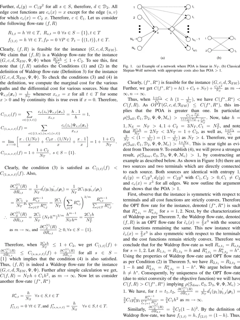
In contrast with the result of [3] that holds for a single source with the edge cost splitting mechanism used above, from Theorem 7, we can note that for most reasonable cost splitting mechanisms, the POA will not equal one for all monomial edge cost functions. We construct explicit examples for POA >1in the Figure 1. The example in Figure 1(a) is near tight as will be evident from an upper bound on POA derived in Theorem 9.
It is interesting to note that in the case when sources are independent, in the Waldrop or OPT solutions, the rates requested at various sources will equal their respective lower bounds (i.e. their entropy). Therefore, the cost term corre-sponding to the sources will be fixed, and one only needs to find flows that minimize the edge costs. In this situation, it is not hard to see that the POA will again equal one for all monomial edge cost functions. i.e. it is the correlation among
the sources that is responsible for bringing more anarchy. We
formalize this below.
Let Ck = {c : ce(x) = aexk, ae > 0,∀e ∈ E} be
the set of edge cost functions where all edge cost functions are monomial of the same degree k possibly with different coefficients, and Cmon = ∪k≥1Ck. Similarly, Dk = {d :
di(y) = bixk, bi > 0,∀s ∈ S}. Also, let Dconvex = {d :
di is convex∀i∈S}.
Corollary 8: Correlation Induces Anarchy: Letze(xe) =
P t∈Txne,t 1n, Ψ e,t(xe) = xn e,t (P j∈Txne,j) , ys(ρs) = P t∈TRms,t m1, andΦ s,t(ρs) = NT1 , then we have
1) ρ(Gall,Cmon,Dconvex,Ψ,Φ,Mind) = 1.
2) ρ(Gall,CNT,Dconvex,Ψ,Φ,Mc) = 1.
3) ρ(Gall,Cmon,Dconvex,Ψ,Φ,Mc) > 1 for large values
ofmandn. In fact,ρ(Gall,C1,D2,Ψ,Φ,Mc)>1+5NT.
4) ρ(Gdsw,Cmon,Dconvex,Ψ,Φ,Mc)>1 for large values
ofmandn.
Proof: Let c ∈ Cmon i.e. ce(x) = aexk for ae > 0
for all e ∈ E, therefore, R cex(x)dx = R
aexk−1 dx =
ae1kxk = 1kce(x). Also, d ∈ Dconvex. Now, since the
sources are independent (i.e. RSW ∈ Mind), from
The-orem 7 and Corollary 6 it follows that a Waldrop flow-rate for instance (G, c, d,RSW,Ψ,Φ) is also an OPT flow-rate for the instance (G, c, d,RSW) which implies that ρ(Gall,Cmon,Dconvex,Ψ,Φ,Mind) = 1.
Even if the sources are correlated, when we havek=NT,
we have NTR cex(x)dx = ce(x) and using Theorem 7, a
Waldrop flow-rate for instance(G, c, d,RSW,Ψ,Φ)is also an OPT flow-rate for the instance (G, c, d,RSW) which implies thatρ(Gall,CNT,Dconvex,Ψ,Φ,Mc) = 1.
We prove ρ(Gall,C1,D2,Ψ,Φ,Mc) > 1+5NT and
conse-quently ρ(Gall,Cmon,Dconvex,Ψ,Φ,Mc) > 1, by explicitly
constructing an example as provided in Figure 1(a). All sources are identical with entropy h, therefore, RSW ∈ Mc.
Further, ds(y) =C1y2 for all s∈S, therefore,d∈D2. All
edge cost functions are ce(x) =xexcept for the edge(u, v)
for which ce(x) =C2 x. Therefore,c ∈C1. Let us consider
the following flow-rate (f, R)
R1,t=h∀t∈T, Rs,t= 0 ∀s∈S− {1}, t∈T
f(1,t)=h∀t∈T, fP = 0∀P ∈Pt− {(1, t)}, t∈T.
Clearly, (f, R) is feasible for the instance (G, c, d,RSW). We claim that (f, R) is a Waldrop flow-rate for the instance (G, c, d,RSW,Ψ,Φ) when 2NTC1h ≤1 +C2. To see this, first
note that (f, R) satisfies the Conditions (1) and (2) in the definition of Waldrop flow-rate (Definition 3) for the instance (G, c, d,RSW,Ψ,Φ). To check the conditions (3) and (4) in the definition, we compute the marginal cost for the various paths and the differential cost for various sources. Note that Ψe,t(xe) = NT1 whenever xe,t = x for all t ∈ T for some
x >0and by continuity this is true even if x= 0. Therefore,
C(1,t)(f) = X e∈{(1,t)} ce(ze)Ψe,t(xe) xe,t =h .1 h = 1, C(1,u,v,t)(f) = X e∈{(1,u),(u,v),(v,t)} ce(ze)Ψe,t(xe) xe,t = lim x−→0 x .(1/N T) x + C2x .(1/NT) x + x .1 x = 1 +1 +C2 NT , C(s,u,v,t)(f) = 1 + 1 +C2 NT , s∈S− {1}.
Clearly, the condition (3) is satisfied as C(1,t)(f) <
C(1,u,v,t)(f). Also, ∂CS(t)(R) ∂Ri,t = 1 NT d′i(yi)y ′ i,t(ρi) = 1 NT 2C1yiy ′ i,t(ρi) =2C1 NT y2i Rm−1 i,t P j∈TRmi,j =2C1 NT X j∈T Rmi,j !2/m Rm−1 i,t P j∈TRmi,j . ∴ ∂C (t) S (R) ∂R1,t = 2C1 NT (NThm)2/m h m−1 NThm =2C1h N2 T asm→ ∞, and ∂C (t) S (R) ∂Rs,t ≥0,∀s∈S− {1}. Therefore, when 2C1h NT ≤ 1 + C2, we get C(1,t)(f) + ∂CS(t)(R) ∂R1,t ≤ C(s,u,v,t)(f) + ∂CS(t)(R) ∂Rs,t for all s ∈ S −
{1} which implies that the condition (4) is also satisfied. Thus, (f, R) is indeed a Waldrop flow-rate for the instance (G, c, d,RSW,Ψ,Φ). Further after simple calculation we get, C(f, R) = NTh+C1h2, as m → ∞. Now let us consider
another flow-rate(f∗, R∗) R∗s,t= h NS ∀s∈S, t∈T f(1∗,t)= 0∀t∈T,andf(∗s,u,v,t)= h NS ∀s∈S, t∈T. u v 1 2 NS-1 NS t1 t1 tNT- 1 t N{T} (a) 1 2 t1 t2 (b)
Fig. 1. (a) Example of a network where POA is linear inNT. (b) Classical Slepian-Wolf network with appropriate costs also has POA>1.
Clearly,(f∗, R∗)is feasible for the instance(G, c, d,RSW). Further, we getC(f∗, R∗) =h(1 +C2+NT) + C1h 2 NS as m→ ∞, n→ ∞. Thus, when 1+C2 C1 < h (1− 1 NS), we have C(f ∗, R∗) < C(f, R). As OP T(G, c, d,RSW) ≤ C(f∗, R∗), this im-plies that the POA is greater than one. In particular, ρ(Gall,C1,D2,Ψ,Φ,Mc) > C1+ NT h 1+C2+NT h + C1 NS . Now, take h = 1, NS = NT > 4,1 + C2 = 3NT, C1 = NT2, and note that 2C1h NT = 2NT < 3NT = 1 +C2, as well as, 1+C2 C1 = 3 NT <(1− 1 NT) = (1− 1 NS)as NT >4. Therefore, we get
ρ(Gall,C1,D2,Ψ,Φ,Mc)> 1+5NT. This is near tight as
evi-dent from Theorem 9. To establish (4), we will prove a stronger result, ρ(Gdsw,C3,D3,Ψ,Φ,Mc) > 1, by constructing an
example as described below. As shown in Figure 1(b) there are two sources and two terminals which are directly connected to each source. Both sources are identical with entropy 1, d1(y) = C1y3, d2(y) = C2y3 with C1, C2 > 0, C1 6= C2
and ce(x) =x3 for all edges. We now outline the argument
that shows that the POA >1.
First, observe that the instance is symmetric with respect to terminals and all cost functions are strictly convex. Therefore the OPT flow rate for the instance, denoted (f∗, R∗) is such thatR∗s,t1 =R
∗
s,t2 fors= 1,2. Next, by the characterization of Waldrop as per Theorem 7, the Waldrop flow-rate, denoted (f, R) is an OPT flow-rate for ˜ce(x) = 23x3 with the source
cost functions remaining the same. This new instance with ˜
ce(x) = 23x3 is also symmetric with respect to the terminals
and the cost functions remain strictly convex. Therefore we conclude that for the Waldrop flow-rate as wellRs,t1 =Rs,t2 fors= 1,2. LetR1,t1 =R1,t2 =handR
∗
1,t1 =R
∗
1,t2 =h
∗.
Using the properties of Waldrop flow-rate and OPT flow rate as per Condition (2) in Theorem 5, we haveR2,t1 =R2,t2 = 1−h and R∗2,t1 = R∗1,t2 = 1−h∗. We argue below that h 6= h∗. Consequently, by uniqueness of the OPT flow-rate (due to strict convexity of the objective function) we will have C(f, R)> C(f∗, R∗)implyingρ(Gdsw,C3,D3,Ψ,Φ,Mc)> 1. We have, for t = t1, t2, ∂C (t) S (R) ∂R1,t = 1 NTd ′ 1(y1)y ′ 1,t(ρ1) = 3 2C1y 2 1y1 Rm−1 1,t P2 j=1Rm1,j = 3 4C1h 2 asm→ ∞. Similarly, ∂C (t) S (R) ∂R2,t = 3 4C2(1−h)2. By the definition of
C(1,t)(f) = h2, C(2,t)(f) = (1−h)2. Further, ∂C(St)(R) ∂R1,t + C(1,t)(f) = ∂CS(t)(R) ∂R2,t +C(2,t)(f)implies that 3 4C1h 2+h2= 3 4C2(1−h) 2+ (1−h)2. Therefore, h 1−h = r 3 4C2+1 3 4C1+1. Now, from Theorem 7, (f∗, R∗) is a Waldrop flow-rate for the instance where everything remains the same except for the edge cost functions which are now 32x3instead ofx3and per-forming the similar calculations as above for(f, R), we obtain
h∗ 1−h∗ = r3 4C2+ 3 2 3 4C1+32
. Clearly, since C1 6=C2, we get h6=h∗.
In particular, take C1 = 4, C2 = 8, then h = 0.5695 and
h∗ = 0.5635. Thus, C(f, R) = 1.9061, C(f∗, R∗) = 1.9052 implying thatP OA≥1.004>1, in this example.
We now state an upper bound that is nearly attained by the example of Figure 1(a).
Theorem 9: Let ze(xe) = Pt∈Txne,t
n1 ,Ψ e,t(xe) = xn e,t (P j∈Txne,j) and Φs,t(ρs) = NT1 . Then,
ρ(Gall,Ck,Dconvex,Ψ,Φ,Mc)≤max{NTk ,NTk }.
Proof: Omitted due to lack of space.
Now we consider another splitting mechanismΦthat looks more like the edge cost splitting mechanism Ψ. Specifi-cally, take ys(ρs) = P t∈T(Rs,t)m 1 m and Φ i,t(ρs) = (Ri,t)m P
j∈T(Rj,t)m. Arguing in a manner similar to Corollary 8(1)
(rates need to equal their corresponding entropies) we ob-tain ρ(Gall,Cmon,Dconvex,Ψ,Φ,Mnc) = 1. Now, we will
argue that with ys(ρs) =
P t∈T(Rs,t)m m1 andΦ i,t(ρs) = (Ri,t)m P j∈T(Rj,t)m we haveρ( Gdsw,Cmon,Dconvex,Ψ,Φ,Mc)>1
for large values of m and n. Let us consider the same example as in Figure 1(b) but with the new source cost splitting mechanism. The previously calculated OPT flow-rate for this instance (f∗, R∗) is given by R∗
1,t = f(1∗,t) = h∗
and R∗
2,t =f(2∗,t) = 1−h∗. We will argue that this is not a
Waldrop flow-rate and since the OPT flow-rate is unique (by strict convexity) we will obtainP OA >1. After some simple calculations we get ∂CS(t)(R) ∂Ri,t =d′i(yi) yi Ri,t Φ2i,t(ρi) +m di(yi) Ri,t Φi,t(ρi) (1−Φi,t(ρi)). Therefore, ∂C (t) S (R ∗ ) ∂R1,t = (m + 3)(NT) 3/m C1 4 (h∗)2 and ∂C (t) S (R ∗ ) ∂R2,t = (m + 3)(NT) 3/m C2 4 (1 − h ∗)2. Also, C(1,t)(f∗) = (h∗)2 and C(1,t)(f∗) = (1 − h∗)2. Note
that NT = 2 in this example. Now, with C1 =
4, C2 = 8, we have h∗ = 0.5635 and therefore
C(1,t)(f∗)+ ∂CS(t)(R∗) ∂R1,t C(2,t)(f∗)+ ∂CS(t)(R∗) ∂R2,t = (h ∗ )2+(m+3)(NT)3/m C1 4 (h ∗ )2 (1−h∗)2+(m+3)(NT)3/m C2 4 (1−h ∗)2 = (m+3)(NT)3/m+1 2(m+3)(NT)3/m+1 0.56352 (1−0.5635)2 = 12 0.5635 2 (1−0.5635)2 = 0.83336= 1 as m→ ∞. REFERENCES
[1] R. Ahlswede, N. Cai, S.-Y. Li, and R. W. Yeung. Network Information Flow. IEEE Trans. on Info. Th., 46, no. 4:1204–1216, 2000.
[2] J. Barros and S. Servetto. Network Information Flow with Correlated Sources. IEEE Trans. on Info. Th., 52:155–170, Jan. 2006.
[3] S. Bhadra, S. Shakkottai, and P. Gupta. Min-Cost Selfish Multicast With Network Coding. IEEE Trans. on Info. Th., 52, no. 11:5077–5087, 2006. [4] S. Boyd and L. Vandenberghe. Convex Optimization. Cambridge
University Press, 2004.
[5] T. Cover and J. Thomas. Elements of Information Theory. Wiley Series, 1991.
[6] R. Cristescu, B. Beferull-Lozano, and M. Vetterli. Networked Slepian-Wolf: theory, algorithms, and scaling laws. IEEE Trans. on Info. Th., 51, no. 12:4057–4073, 2005.
[7] S. C. Dafermos and F. T. Sparrow. The traffic assignment problem for a general network. J. Res. Nat. Bureau of Standards, Series B, 73B(2):91– 118, 1969.
[8] T. Ho, M. M´edard, M. Effros, and R. Koetter. Network Coding for Correlated Sources. In Conf. on Information Sciences and Systems, 2004.
[9] E. Koutsoupias and C. H. Papadimitriou. Worst-case equilibria. In STACS, pages 404–413, 1999.
[10] Z. Li. Min-Cost Multicast of Selfish Information Flows. In Proc. of IEEE INFOCOM, 2007.
[11] Z. Li. Cross-Monotonic Multicast. In Proc. of IEEE INFOCOM, 2008. [12] Z. Li and B. Li. Efficient and Distributed Computation of Maximum
Multicast Rates. In Proc. of IEEE INFOCOM, 2005.
[13] D. S. Lun, N. Ratnakar, M. M´edard, R. Koetter, D. R. Karger, T. Ho, E. Ahmed, and F. Zhao. Minimum-Cost Multicast over Coded Packet Networks. IEEE Trans. on Info. Th., 52:2608–2623, June 2006. [14] C. B. M. M Beckman and C. B. Winsten. Studies in the Economics of
Transportation. Yale University Press, New Haven,CT, 1956. [15] N. Nisan, T. Roughgarden, E. Tardos, and V. V. Vazirani. Algorithmic
Game Theory. Cambridge University Press, New York, NY, USA, 2007. [16] M. J. Osborne and A. Rubinstein. A Course in Game Theory. The MIT
Press, Cambridge, MA, USA, 1994.
[17] C. H. Papadimitriou. Algorithms, games, and the internet. In STOC ’01: Proceedings of the thirty-third annual ACM symposium on Theory of computing, pages 749–753, New York, NY, USA, 2001. ACM. [18] V. Prabhakaran, D. Tse, and K. Ramchandran. Rate Region of the
quadratic Gaussian CEO problem. In IEEE Intl. Symposium on Info. Th., pages 119–119, 2004.
[19] A. Ramamoorthy. Minimum cost distributed source coding over a network. In IEEE Intl. Symposium on Info. Th., pages 1761–1765, 2007. [20] T. Roughgarden. Selfish Routing and the Price of Anarchy. The MIT
Press, 2005.
[21] T. Roughgarden and ´Eva Tardos. How bad is selfish routing? J. ACM, 49(2):236–259, 2002.
[22] D. Slepian and J. Wolf. Noiseless coding of correlated information sources. IEEE Trans. on Info. Th., 19:471–480, Jul. 1973.
[23] R. Zamir and T. Berger. Multiterminal source coding with high resolution. IEEE Trans. on Info. Th., 45, no. 1:106–117, 1999.
APPENDIX
Lemma 10: LetRt∈RSWi.e.Pl∈ARl,t≥H(XA|X−A)
for all A ⊆ S. If S1, S2 ∈ S satisfy Pl∈S1Rl,t = H(XS1|X−S1) and P l∈S2Rl,t = H(XS2|X−S2) then we have P l∈S1∩S2Rl,t = H(XS1∩S2|X−(S1∩S2)) and P l∈S1∪S2Rl,t=H(XS1∪S2|X−(S1∪S2)). Proof: We have, P l∈S1∩S2Rl,t + P l∈S1∪S2Rl,t = P l∈S1Rl,t + P l∈S2Rl,t = H(XS1|X−S1) + H(XS2|X−S2) ≤ H(XS1∩S2|X−(S1∩S2)) + H(XS1∪S2|X−(S1∪S2))where in the second step we have used the supermodularity property of conditional entropy. Now we are also given that P
l∈S1∩S2Rl,t ≥H(XS1∩S2|X−(S1∩S2)) and P
l∈S1∪S2Rl,t ≥ H(XS1∪S2|X−(S1∪S2)). Therefore we can conclude that P
l∈S1∪S2Rl,t ≤ H(XS1∪S2|X−(S1∪S2)) and P l∈S1∩S2Rl,t ≤ H(XS1∩S2|X−(S1∩S2)) and consequently that P l∈S1∪S2Rl,t = H(XS1∪S2|X−(S1∪S2)) andP l∈S1∩S2Rl,t=H(XS1∩S2|X−(S1∩S2)).