Variable Sized Bin Packing Problem
Christian Blum1, Vera Hemmelmayr2, Hugo Hern´andez1, and Verena Schmid2
1 ALBCOM Research Group, Universitat Polit`ecnica de Catalunya, Barcelona, Spain {cblum,hhernandez}@lsi.upc.edu
2 Department of Business Administration, Universit¨at Wien, Vienna, Austria {vera.hemmelmayr,verena.schmid}@univie.ac.at
Abstract. This paper deals with the so-called variable sized bin packing problem, which is a generalization of the one-dimensional bin packing problem in which a set of items with given weights have to be packed into a minimum-cost set of bins of variable sizes and costs. First we propose a heuristic and a beam search approach. Both algorithms are strongly based on dynamic programming procedures and lower bounding techniques. Second, we propose a variable neighborhood search approach where some neighborhoods are also based on dynamic programming. The best results are obtained by using the solutions provided by the proposed heuristic as starting solutions for variable neighborhood search. The results show that this algorithm is very competitive with current state-of-the-art approaches.
1
Introduction
The variable sized bin packing problem (VSBPP) is a generalization of the well-known one-dimensional bin packing packing (BPP). The objective consists of packing a set of given items into a minimum-cost set of bins of variable sizes and costs. Practical applications of the problem arise in packing, transportation planning, and cutting [6]. The literature on the VSBPP offers work on approx-imation algorithms [4,3,8] and exact algorithms [11,2,1,7]. However, even the best-performing exact approaches can only be applied to relatively small prob-lem instances. The best algorithms for larger probprob-lem instances were proposed by Haouari and Serairi in [6]. After introducing a range of greedy heuristics, Haouari and Serairi also presented a genetic algorithm. They applied their algo-rithms to two sets of problem instances. While the genetic algorithm was best for linear-cost instances, a heuristic based on set covering performed better for other types of instances.
This work was supported by the binational grant Acciones Integradas ES16-2009 (Austria) and MEC HA2008-0005 (Spain), and by grant TIN2007-66523 (FOR-MALISM) of the Spanish government. In addition, Christian Blum acknowledges support from theRam´on y Cajal program of the Spanish Government of which he is a research fellow, and Hugo Hern´andez acknowledges support from the Catalan Government through anFI grant.
M.J. Blesa et al. (Eds.): HM 2010, LNCS 6373, pp. 16–30, 2010. c
In this paper we propose hybrid algorithms based on dynamic and linear programming techniques. First, we introduce a heuristic and a beam search approach, both based on dynamic programming procedures and bounding tech-niques. In addition to evaluating them as stand-alone-approaches, both algo-rithms are also used for providing high-quality starting solutions to a variable neighborhood search algorithm. As we will show, the combination of our heuristic with variable neighborhood search obtains the best results, beating or equalling the results of the best algorithms from the literature on two sets of problem instances.
The organization of this work is as follows. The VSBPP is technically pre-sented in Section 2. While the proposed heuristic and beam search are outlined and experimentally evaluated in Section 3, the same is done for variable neigh-borhood search in Section 4. Finally, in Section 5 we offer conclusions and an outlook to future work.
2
Variable Sized Bin Packing
The VSBPP can be formally defined as follows. Given is a set S of n items,
S ={1, . . . , n}. Each itemi∈ S has a weight wi >0. Furthermore, given is a
setB of mdifferent bin types,B={1, . . . , m}, where each bin typek∈B has
a capacity Wk > 0 and a cost ck. Without loss of generality we assume that
W1< . . . < Wm. The goal is to pack thenitems into a number of bins such that the sum of the costs of the bin types is minimized. In the following we present an integer programming model for the VSBPP. This model includes two sets
of binary variables. A variablexij ∈ {0,1} is set to 1, that is,xij = 1, in case
itemiis placed in binj. Note that we assume here that maximallynbins may
be used. In this extreme case each item is packed into its own bin. Moreover, a
variableyjk ∈ {0,1} is set to 1, that is,yjk = 1, in case binj has bin type k.
With these variables the VSBPP can be expressed as follows. min n j=1 m k=1 ck·yjk (1) subject to: n j=1 xij = 1 fori= 1, . . . , n (2) m k=1 yjk≤1 forj = 1, . . . , n (3) n i=1 wi·xij ≤ m k=1 Wk·yjk forj= 1, . . . , n (4) xij ∈ {0,1} fori, j= 1, . . . , n (5) yjk ∈ {0,1} forj = 1, . . . , nandk= 1, . . . , m (6)
Note that, as a generalization of the one-dimensional bin packing problem, the VSBPP is NP-hard.
3
A Heuristic and Beam Search for the VSBPP
The two algorithms that we propose in the following are strongly based on dynamic programming and/or lower bounding techniques. First we introduce a heuristic that uses lower bounding techniques as greedy information. Then we describe a beam search (BS) approach, which is a heuristic variant of branch & bound introduced in the context of scheduling problems [12]. The central idea of BS is the parallel construction of several solutions guided by two crucial algorithmic components, a greedy heuristic and a lower bound.
3.1 The SSP3 Heuristic from the Literature
As mentioned already in the introduction, Haouari and Serairi [6] proposed a range of greedy heuristics for the VSBPP. The best balance between speed and quality is obtained by a heuristic labeled SSP3 in [6], which works as follows. SSP3 iteratively fills one bin after the other until no unpacked items are left. In the context of SSP3 (and beam search) we henceforth denote (partial) solutions
to the VSBPP as sequences t = t1. . . t|t|, where ti ∈ B for all i = 1, . . . ,|t|.
In other words, a (partial) solution is represented by an ordered sequence of bin types. The interested reader may note that in the context of SSP3 such a representation is well-defined. At each iteration of SSP3, given a partial solution
t, let us denote bySt⊆Sthe set of unpacked items, that is,S\Stare the items
that are packed into the|t|bins of partial solutiont. Two design decisions have
to be made: (1) a bin type must be chosen, and (2) the set of items that will
be packed into the new bin have to be selected fromStwith the condition that
the heaviest remaining item—that is, argmax{wi|i∈St}—is among the chosen
items. Due to this condition, only bin typesk withWk ≥max{wi|i∈St}may
be considered. Let us denote the bin type with the smallest feasible capacity by
kmin. The feasible extensions of a partial solution t are all sequences tk where
k ∈ {kmin, . . . , m}. The greedy value η(tk) of an extension tk is calculated as follows. First, the following NP-hard subset sum problem is solved in pseudo-polynomial time by dynamic programming [9]:
zk :=max i∈St wi·xi (7) subject to: i∈St wi·xi≤Wk (8) xi ∈ {0,1} fori∈St (9)
Apart from the value zk of the calculated optimal solution, let us denote by
Ik ⊆ St the set of items that corresponds to this optimal solution, that is,
Ik :={i∈St|xi = 1}. The greedy value oftk is then defined asck/zk, that is,
η(tk) :=ck/zk. At each step SSP3 chooses the bin type k∗ ∈ {kmin, . . . , m}for
whichη(tk∗) is minimal. The algorithm stops once all items are packed, that is,
whenSt=∅.
3.2 Lower Bound
In the following we will denote the objective function value of a (partial) solution
t by f(t) := |t|i=1cti. Six different lower bounds for the VSBPP have been
proposed in [7] in the context of a branch & bound algorithm. We implemented
two of them. The first one, labeled L0 in [7], is a simple problem relaxation
which is obtained by allowing items to be split. However, this relaxation itself is NP-hard and the corresponding integer program was solved with CPLEX.
Given a partial solutiont, let us denote the corresponding value byL0(t). The
second bound that we chose, labeled L3 in [7], is an NP-hard bound based on
network flows. Also in this case the corresponding integer program was solved
with CPLEX. With respect to a partial solution t, the corresponding value is
denoted byL3(t).
3.3 The Lower Bound Heuristic
The lower bound heuristic (LBH) is obtained as a variant of SSP3 as follows. Instead of the original definition of the greedy values, LBH uses the following
redefinition. Each feasible extension tk of a partial solution t has the greedy
valueη(tk) :=f(tk) + LB(tk), where LB(·) refers either to lower boundL0or to
lower boundL3.
3.4 The BS Algorithm
The implemented BS algorithm, which is based on the previously described heuristics and the lower bounds, works as follows. At each step, the algorithm
chooses at mostμkbwfeasible extensions of the partial solutions stored in a set
B, known as thebeam. Hereby,kbwis the so-calledbeam widththat limits the size
ofB, andμ≥1 is a parameter of the algorithm. The choice of feasible extensions
is done deterministically based on the greedy function outlined in Section 3.1.
At the end of each step, the algorithm creates a new beamB by selecting up to
kbwpartial solutions from the set of chosen feasible extensions. For this purpose,
each chosen extension is evaluated on the basis of its lower bound value. Only
the maximallykbwbest extensions—with respect to this evaluation—are chosen
for the new beamB. Finally, the best found complete solution is returned.
We next explain the functions of Algorithm 1 in detail. The algorithm uses four
different functions. Hereby, function LowerBoundHeuristic() executes heuristic
Algorithm 1.Beam search (BS) for the VSBPP 1: input:a problem instance
2: Bcompl:=∅,B:={∅} 3: tbsf:=LowerBoundHeuristic() 4: whileB=∅do 5: C:=Produce Extensions(B) 6: B:=∅ 7: fork= 1, . . . ,min{μkbw,|C|}do 8: tk:=Choose Best Extension(C) 9: if Stk=∅then 10: Bcompl :=Bcompl∪ {tk} 11: if f(tk)< f(tbsf)thentbsf:=tkend if 12: else 13: if f(t) +UB(tk)≤f(tbsf)thenB:=B∪ {tk}end if 14: end if 15: C:=C\ {tk} 16: end for 17: B:=Reduce(B, kbw) 18: end while
19: output:argmin{f(t)|t∈Bcompl}
functionProduce Extensions(B) produces the setC of feasible extensions of all
sequences in B. More specifically, C is the set of sequences tk, where t ∈ B
andk∈ {kmin, . . . , m}. The third function,Choose Best Extension(C), is used for
choosing extensions fromC. In this context note that for the comparison of two
extensionstk and tk fromC the greedy function is only useful in caset=t,
while it might be misleading in caset =t. We solved this problem as follows.
First, instead of the greedy weightsη(), we use the corresponding ranks. More
specifically, given all feasible extensions{tk |k ∈ {kmin, . . . , m}} of a sequence
t, the extension tk with η(tk)≤η(tk) for allk ∈ {kmin, . . . , m} receives rank
1, denoted byr(tk) = 1. The extension with the second smallest greedy weight
receives rank 2, etc. For evaluating an extension tk we then use the sum of
the ranks of the greedy weights that correspond to the well-defined sequence of
construction steps that were performed to construct sequencetk, that is
ν(tk) :=r(t1) + ⎛ ⎝|t|− 1 i=1 r(t1· · ·titi+1) ⎞ ⎠+r(tk) (10)
wheret1· · ·tidenotes the subsequence oftfrom position 1 to positioni, andti+1
denotes the bin type at position i+ 1 of sequencet. In contrast to the greedy
function weights, these newly definedν()-values can be used to compare
exten-sions of different sequences. In fact, a call of functionChoose Best Extension(C)
returns the extension fromC with minimalν() value.
Finally, the last function used by the BS algorithm is Reduce(B, kbw). This
function reduces B to the best kbw sequences with respect to an evaluation
For any sequencet∈Bthe evaluation measure is defined asf(t) + LB(t), where
f(t) refers to the objective function value of the partial solution t, and LB(t)
either refers to the lower bound valueL0(t) orL3(t), depending on which of the
two lower bounds is used by BS.
3.5 Experimental Evaluation of LBH and BS
Both the LBH and BS were implemented in C++ and experimentally evaluated on a cluster of PCs equipped with Pentium D processors with 3.2 GHz. For
computing the lower boundsL0 andL3 we used CPLEX 12.1. Two benchmark
sets from the literature were used for testing. Set1 consists of ten instances for
eachn∈ {25,50,100,200,500}, wherenis the number of items. Moreover, these
instances are linear-cost instances, that is,Wi =ci for alli∈ {1, . . . , m}, where
m = 3 for all instances. The capacities, respectively costs, were chosen to be
W1 = 100,W2 = 120 andW3 = 150. Item weights were randomly drawn from
[1,100]. These 50 instances were originally proposed in [11]. The second instance
set, henceforth denoted by Set2, was proposed in [6]. For all the instances from
Set2, the number of bin types (m) was set to 7 and capacities were defined
as W1 = 70, W2 = 100, W3 = 130, W4 = 160, W5 = 190, W6 = 220 and
W7= 250. Moreover, item weights were randomly drawn from [1,250]. Finally,
these instances split into three different classes, where class B1 is characterized
by a linear cost function ci = Wi (i = 1, . . . ,7), class B2 has a concave cost
functionci =10√Wi(i= 1, . . . ,7), and class B3 has a convex cost function
ci=0.1Wi3/2(i= 1, . . . ,7). Set2 consists of 10 instances for each combination
ofn(number of items) and class. This makes a total of 150 problem instances.
The following five algorithm versions were applied to Set1 and Set2: LBH(L0),
respectively LBH(L3), denotes the lower bound heuristic using L0, respectively
L3, as bounding technique. Furthermore, BS(L0), respectively BS(L3), denotes
beam search using L0, respectively L3, as lower bound. Note that parameter
settings kbw = 10 and μ = 4.0 were used for these versions of BS. Finally, we
also tested algorithm BS(L0, kbw = 100), that is, BS using L0 as lower bound
and using a beam width of 100. These five algorithm versions were compared to the two best algorithms proposed in [6]: Algorithm SC is a heuristic based on set covering, and GEN denotes a genetic algorithm. While GEN is superior to SC for what concerns the instances of Set1, SC is notably better than GEN for the instances of Set2.
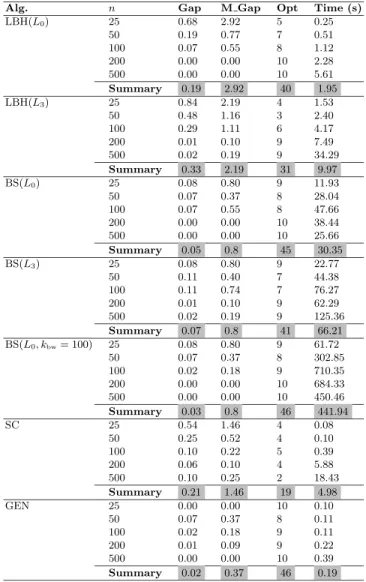
The results of our algorithms for the instances of Set1 are presented in com-parison to SC and GEN in Table 1. The results are presented in the same way
as in [6]. Column Gap presents the average percentage deviation (over 10
in-stances) with respect to the value of the optimal solutions (as computed by a
branch & bound approach from [7]). ColumnM Gapcontains the maximal one
of these gaps (over 10 instances). Furthermore, columnOpt provides the
num-ber of instances (out of 10) that were solved to optimality, and columnTime
(s)presents the average computation times (over 10 instances) in seconds. For
in the columns (for columnsGap andTime (s)), respectively the maxium of
the values in columnM Gapand the sum of the values in columnOpt.
First—and surprisingly—in addition to being faster, the algorithm versions
using lower boundL0 achieve higher solution qualities than the algorithm
ver-sions usingL3. This is despite the fact thatL3 is a tighter lower bound thanL0
(see [7]). Concerning the comparison between LBH and BS, we can state that BS improves—in terms of solution quality—over the corresponding versions of
LBH. For example, while LBH(L0) can solve 40 (out of 50) instances to
optimal-ity, BS(L0) can solve 45 instances to optimality. However, this comes at the cost
of significantly higher computation times. Moreover, increasing the beam width
(kbw) in BS does not seem to be very beneficial. Even though the algorithm
slightly improves in terms of solution quality, this is not justified by the increase in computation time requirements. For what concerns the comparison to SC
and GEN, we note that both LBH(L0) and BS(L0) are superior to SC in terms
of solution quality. However, while the performance of BS(L0) is comparable,
in terms of solution quality, to the one of GEN, LBH(L0) is clearly inferior to
GEN. The great advantage of GEN in comparison to both LBH(L0) and BS(L0)
are the low computation time requirements. In this context, note that both SC and GEN were executed on a PC with a Pentium IV (3.2 GHz) processor and 2 GB of RAM, which should be comparable in speed to the machines that we used.
The computational results for Set2 are presented in Table 2. As the compar-ison between our five algorithm versions was basically the same as for Set1, we
only show the results of LBH(L0) and BS(L0). Moreover, these two algorithm
versions are henceforth simply denoted by LBH and BS. Note also that the for-mat of Table 2 is slightly different to the one of Table 1. First, optimal solutions are not known for the instances of Set2. Therefore, instead of referring to
opti-mal solutions, columns Gap and M Gapnow refer to the relative percentage
deviation from a lower bound value derived in [7]. Moreover, for the same reason
column Opt does not exist in Table 2. For what concerns the comparison of
LBH and BS to SC and GEN, we must note that both LBH and BS are gen-erally inferior to both SC and GEN. Hereby, this is more pronounced for what concerns instances with a concave and a convex cost function. However, also for the instances with linear cost function LBH and BS are now inferior to SC, which might be related to the increase in the number of bin types as well as to the increase in the number of items.
4
Variable Neighborhood Search
Variable neighborhood search (VNS) is a metaheuristic which has originally been proposed in [10] and extended in [5]. It is an improvement heuristic based on local search and has already been successfully applied to a number of combinatorial optimization problems. In contrast to population-based approaches VNS works at each iteration on a single solution only. An efficient search within the solution space is usually achieved by the use of both diversification and intensification
Table 1. Results of the Lower Bound Heuristic (LBH) and Beam Search (BS) in comparison to SC and GEN for all instances from Set1
Alg. n Gap M Gap Opt Time (s)
LBH(L0) 25 0.68 2.92 5 0.25 50 0.19 0.77 7 0.51 100 0.07 0.55 8 1.12 200 0.00 0.00 10 2.28 500 0.00 0.00 10 5.61 Summary 0.19 2.92 40 1.95 LBH(L3) 25 0.84 2.19 4 1.53 50 0.48 1.16 3 2.40 100 0.29 1.11 6 4.17 200 0.01 0.10 9 7.49 500 0.02 0.19 9 34.29 Summary 0.33 2.19 31 9.97 BS(L0) 25 0.08 0.80 9 11.93 50 0.07 0.37 8 28.04 100 0.07 0.55 8 47.66 200 0.00 0.00 10 38.44 500 0.00 0.00 10 25.66 Summary 0.05 0.8 45 30.35 BS(L3) 25 0.08 0.80 9 22.77 50 0.11 0.40 7 44.38 100 0.11 0.74 7 76.27 200 0.01 0.10 9 62.29 500 0.02 0.19 9 125.36 Summary 0.07 0.8 41 66.21 BS(L0, kbw= 100) 25 0.08 0.80 9 61.72 50 0.07 0.37 8 302.85 100 0.02 0.18 9 710.35 200 0.00 0.00 10 684.33 500 0.00 0.00 10 450.46 Summary 0.03 0.8 46 441.94 SC 25 0.54 1.46 4 0.08 50 0.25 0.52 4 0.10 100 0.10 0.22 5 0.39 200 0.06 0.10 4 5.88 500 0.10 0.25 2 18.43 Summary 0.21 1.46 19 4.98 GEN 25 0.00 0.00 10 0.10 50 0.07 0.37 8 0.11 100 0.02 0.18 9 0.11 200 0.01 0.09 9 0.22 500 0.00 0.00 10 0.39 Summary 0.02 0.37 46 0.19
strategies. During shaking phases the current incumbent solution is perturbed by means of different neighborhood structures, allowing the solution process to explore various regions of the solution space and (hopefully) to escape from local optima. The subsequent use of local search intensifies the search.
A sketch of the basic steps of a standard VNS can be found in Algorithm 2. After the generation of an initial solution, at each iteration the current solution
xis systematically perturbed by means of κmax neighborhood structures Nκ,
where 1≤κ≤κmax. The perturbed solutionx is then locally optimized during
Ta b le 2 . Re su lt s o f the Lo w e r B o und He uri sti c (LB H) a n d B e a m S e a rc h (B S ) in c o m pa ri so n to S C a nd G E N fo r a ll in st a n c e s fro m S e t2 Alg. n Class B 1 C lass B2 Class B 3 Gap M Gap T i m e( s ) G a p M Gap T i m e( s ) G a p M Gap T i m e( s ) LBH 100 1.11 1.86 0.40 1.35 1.98 4.09 2.55 3.53 4.74 200 1.12 1.94 0.78 1.55 2.26 8.59 2.81 3.46 10.10 500 0.60 1.01 1.95 0.91 1.49 21.27 2.93 3.87 19.96 1000 0.48 0.78 3.33 0.76 1.27 33.17 2.86 3.14 35.17 2000 0.36 0.46 7.43 0.53 0.96 52.60 2.86 3.03 68.26 Su mm ary 0.73 1.94 2.78 1.02 2.26 23.94 2.80 3.87 27.65 BS 100 0.96 1.41 215.38 1.30 1.98 181.05 2.40 3.24 481.51 200 1.07 1.83 322.24 1.48 2.21 319.61 2.75 3.46 725.48 500 0.56 0.90 826.85 0.89 1.48 811.87 2.92 3.87 1095.43 1000 0.44 0.78 1817.60 0.70 1.18 1869.34 2.86 3.14 2160.20 2000 0.34 0.43 4798.96 0.52 0.88 4547.01 2.86 3.03 5589.34 Su mm ary 0.68 1.83 1596.21 0.98 2.21 1545.78 2.76 3.87 2010.39 SC 100 0.85 1.41 0.23 1.03 1.83 3.77 2.22 3.08 0.09 200 0.98 1.64 0.22 1.27 2.21 8.69 2.43 3.16 0.17 500 0.46 0.80 3.85 0.71 1.21 12.47 2.56 3.33 0.54 1000 0.37 0.72 5.95 0.62 1.03 19.78 2.51 2.83 1.83 2000 0.32 0.41 12.89 0.44 0.82 21.41 2.50 2.69 6.73 Su mm ary 0.60 1.64 4.63 0.81 2.21 13.22 2.44 3.33 1.87 GEN 100 0.82 1.41 0.85 1.08 1.83 1.11 2.23 3.08 1.06 200 0.95 1.64 1.96 1.32 2.21 1.99 2.57 3.49 1.98 500 0.49 0.79 4.38 0.77 1.32 5.05 2.71 3.55 4.35 1000 0.41 0.76 10.92 0.66 1.13 12.07 2.61 2.89 9.89 2000 0.33 0.43 29.88 0.47 0.86 37.12 2.56 2.83 34.45 Su mm ary 0.60 1.64 9.60 0.86 2.21 11.47 2.54 3.55 10.35
Algorithm 2.A Standard Version of VNS input:a problem instance
x←GenerateInitialSolution() whilestopping criterion not metdo
κ←1 whileκ≤κmaxdo x←Shaking(x, κ) x←LocalSearch(x) if Accept(x, x)then x←x κ←1 else κ←κ+ 1 end if end while end while
output:best solution found
is met,xbecomes the new incumbent solution and the search procedure starts
over again with the first neighborhood structure. Otherwise the search continues
withxas incumbent solution and uses the next neighborhood structureκ+ 1.
In the following we present our implementation of VNS for the VSBPP. In
the context of VNS, a solutionxis an explicit list of bins with their items and
bin types.
4.1 Implementation of VNS for the VSBPP
In order to find a feasible initial solution a suitable bin is randomly chosen for each item. In fact, each item is packed into a separate bin. The selection
proba-bility is directly proportional to the ratio Wk
ck, hence favoring the assignment of
items to bins which have low cost with respect to their capacity.
Shaking. For our shaking step we defined three neighborhood structures. The
first one, henceforth denoted byN1, changes the type of a given number of bins.
The second one (N2) deletes bins and repacks the items, whereas the third one
(N3) is based on dynamic programming. The way in which these three
neighbor-hood structures (or operators) are used is slightly different to the way in which they would be used in the standard VNS that is shown in Algorithm 2. For each of the three operators we keep track of the number of successful applications.
Then, wheneverShaking(x) is applied, the choice of the operator depends on the
performance of the corresponding operator in previous steps. Hereby, the selec-tion probability is directly proporselec-tional to the number of successful applicaselec-tions in the past. In the following we describe the three operators in more detail.
OperatorN1(x) selects up to 15% of all bins currently used by solutionxand
changes their corresponding bin types randomly. In case this produces a binb
bin capacity ends up being too small) items are randomly removed until the capacity of the bin is sufficient. This may generate a set of currently un-packed items, which are sorted in a non-increasing manner with respect to their weight. Then one after the other is inserted into any of the currently open bins. We use a roulette-wheel approach based on the remaining bin capacities, where the selection probability for a bin to be chosen is inversely related to the remaining capacity of the bin. If an item does not fit into any of the bins currently in use, a new bin is added to the solution. The bin type is randomly chosen proportional to the ratio cost/capacity (a small ratio is favored).
OperatorN2(x) chooses up to 5% of all bins of xand deletes them from x.
All items previously assigned to these bins have to be repacked. This is done by assigning each of these items to a new bin whose bin type is randomly chosen among all bin types where the item would fit.
Finally, operator N3(x) uses a packing procedure based on dynamic
pro-gramming proposed in [6]. This dynamic propro-gramming procedure provides the minimum-cost VSBPP solution for a given sequence of items. The given
se-quence imposes that for each itemj that appears after an item i, itemj must
appear either in the same bin asi or in a later bin. In order to obtain such an
item sequence, the items of the bins ofx are appended in the order in which
they appear in x. Hereby, the items of each bin are sorted according to their
weight. The sorting is done either in a non-decreasing or non-increasing way, in an alternating fashion.
Note that the maximal neighborhood sizes (15% of all bins in the case ofN1,
respectively 5% of all bins in the case of N2) were determined after extensive
experimentation.
Local Search. Three different neighborhood structures were used for local search.
The first two (N4 and N5) are based on the intuition that in a (near-)optimal
solution all bins are probably quite densely packed. In other words, the remaining
capacity of all bins used should be rather small. The goal of the operatorsN4and
N5is therefore to obtain densely packed bins. OperatorN4 tries to improve the
capacity usage, that is, it tries to decrease the remaining capacity of each bin by
moving an item from its current binato a different binb. Such a move can only
be executed if the resulting packing is feasible with respect to the corresponding
capacities and if the remaining capacity of binbafter the move is smaller than
the remaining capacity of bina before the move. Hence we try to fill up bins
whose utilization level is already high, while emptying others that are currently
not fully utilized. With a similar intention, operatorN5 tries to swap an item
icurrently packed in binawith an item j currently packed into a different bin
b. The swap is executed if and only if the remaining capacity of binb after the
swap is smaller than the remaining capacity of bin abefore the swap and the
resulting packing is feasible with respect to the bin capacities. As we are urging to obtain densley packed bins, furthermore a swap is only considered feasible if
the remaining capacity of binbdecreases, i.e. ifwi> wj.
After this first phase there tend to be bins that are currently far from be-ing densely packed. Hence, the goal should be to remove those bins. Therefore,
operatorN6selects the bin with the lowest load. All items currently assigned to this bin are tried to be inserted into other bins based on a best fit procedure. In case all items can be removed successfully, the corresponding bin can be deleted from the solution.
In a final step, local search iterates through all bins currently in use and tries to change the corresponding bin types in order to use cheaper bins if possible. The neighborhoods are used sequentially and are executed in a first improvement fashion.
Acceptance Criterion. After the original solution has been perturbed by the shaking operator and the local search phase has been executed, the resulting so-lution is compared to the original soso-lution. It is only accepted as new incumbent solution if the objective function value has been improved.
4.2 Computational Results
We tested three versions of VNS, where different starting solutions have been used. Henceforth we refer to VNS using the simple starting solution (as de-scribed above) by VNS(si). Moreover, the version of VNS that uses the lower bound heuristic (as described in Section 3.3) as starting solution is denoted by VNS(lbh). Finally, the last version of VNS uses beam search (see Section 3.4) as starting solution and is denoted by VNS(bs). Due to the random nature of VNS, each instance was solved five times. The reported results are the average values obtained. The run time limit has been set to 10 seconds for instances of Set1 (small linear-cost instances), and to 100 seconds for the instances of Set2 (larger instances). Remember that the instance sets are described in Section 3.5. VNS was implemented using C++ and has been tested on the same cluster of PCs as LBH and BS. Tables 3 and 4 show the corresponding results for the instances of Set1 and Set2. Note that computation times are given in the form
(X/Y), whereX refers to the time of computing the starting solution andY to
the time of VNS. Both times must be added in order to obtain the total time of the algorithm.
As can be seen, VNS performs very well compared to the algorithms proposed in [6]. The best results obtained improve over – or are at least as good as – the results of GEN (in the case of Set1) and SC (in the case of Set2). Remember that the results of GEN and SC are given in Tables 1 and 2.
As can be seen in Table 3, for the small, linear- cost instances (Set 1), all three versions of VNS find the optimal solutions to all 50 problem instances. Please note that the reported results are averaged values over 5 independent test runs for each instance and that we are able to find the optimal solution in every run. This proves that this algorithm is very stable and robust. Even when using the simple procedure for generating the starting solution, on average the optimal solution was found after 0.75 seconds. The algorithms SC (GEN) proposed in [6] need on average 4.98 (0.19) seconds for generating their best solution. Also note that SC (GEN) find the optimal solution in only 19 (46) out of 50 instances.
Table 3.Results of VNS with different starting solutions for all instances from Set1
Alg. n Gap M Gap Opt Time (s)
VNS(si) 25 0.00 0.00 10 (0.00/0.08) 50 0.00 0.00 10 (0.00/0.57) 100 0.00 0.00 10 (0.00/0.16) 200 0.00 0.00 10 (0.00/0.33) 500 0.00 0.00 10 (0.00/2.62) Summary 0.00 0.00 50 (0.00/0.75) VNS(lbh) 25 0.00 0.00 10 (0.25/0.09) 50 0.00 0.00 10 (0.51/0.72) 100 0.00 0.00 10 (1.12/0.15) 200 0.00 0.00 10 (2.28/0.00) 500 0.00 0.00 10 (5.61/0.00) Summary 0.00 0.00 50 (1.95/0.19) VNS(bs) 25 0.00 0.00 10 (11.93/0.11) 50 0.00 0.00 10 (28.04/0.73) 100 0.00 0.00 10 (47.66/0.18) 200 0.00 0.00 10 (38.44/0.00) 500 0.00 0.00 10 (25.66/0.00) Summary 0.00 0.00 50 (30.35/0.20)
For the set of larger instances (Set2) our algorithm improves over the results of the so-far best algorithm SC for what concerns the linear and convex cost classes (class B1 and B3). Moreover, it produces comparable results for class B2. For class B1 the average (maximum) gap obtained by the algorithms of [6] is 0.6% (1.64%). The VNS using the simple initial solution (si) yields an average gap that is slightly worse (0.62%). When initializing the VNS with the more sophisticated initial solutions (provided by LBH and BS) the average gap can be reduced to 0.58%. However, only version VNS(lbh) is practical due to the high computation time requirements of beam search. Furthermore, notice that all proposed procedures obtain the same maximum gap. For class B2 we obtain the same results as in [6]. Again, starting from a more sophisticated initial solution is beneficial for the solution quality. For class B3, all three versions of VNS are able to improve the average as well as the maximum gap found by [6]. The average (maximum) gap of the VNS is 2.43% (3.29%), while the resulting gaps of the best algorithms from [6] amount to 2.44% (3.33%).
Concerning computation times, note that our algorithms are generally slower than both SC and GEN. However, in absolute terms, the computation times of VNS(si) and VNS(lbh) are still quite low. Moreover, note that the authors of [6] have experimentally shown that GEN is not able to improve when given more computation time. Also remember that SC is a deterministic heuristic, which means that it can not benefit from additional computation time either.
Summarizing, our best algorithm version is able to provide high quality so-lutions for both sets of instances, whereas the performance of the algorithms provided in [6] is instance-dependent. For Set1 GEN outperforms SC, whereas for Set2 the performance is vice versa.
Ta b le 4 . R e su lt s o f V N S wit h d iff e ren t st art in g solu ti on s for all in st a n c es from S e t2 Alg. n Class B 1 C lass B2 Class B 3 Gap M Gap T i m e( s ) G a p M Gap T i m e( s ) G a p M Gap T i m e( s ) VNS(si) 100 0.79 1.41 (0.00/14.40) 1.00 1.83 (0.00/3.12) 2.21 3.08 (0.00/0.37) 200 0.93 1.64 (0.00/13.59) 1.26 2.21 (0.00/21.91) 2.40 3.16 (0.00/7.59) 500 0.50 0.79 (0.00/46.99) 0.80 1.40 (0.00/40.05) 2.54 3.29 (0.00/49.11) 1000 0.45 0.79 (0.00/61.17) 0.89 1.45 (0.00/59.35) 2.49 2.82 (0.00/76.60) 2000 0.45 0.60 (0.00/87.84) 0.79 1.12 (0.00/86.33) 2.49 2.69 (0.00/89.69) Su mm ary 0.62 1.64 (0.00/44.80) 0.95 2.21 (0.00/42.15) 2.43 3.29 (0.00/44.67) VNS(lbh) 100 0.79 1.41 (0.40/12.84) 1.00 1.83 (4.09/4.71) 2.21 3.08 (4.74/0.22) 200 0.93 1.64 (0.78/7.24) 1.23 2.21 (8.59/10.39) 2.40 3.16 (10.10/14.09) 500 0.47 0.77 (1.95/20.46) 0.70 1.25 (21.27/10.48) 2.54 3.29 (19.96/45.69) 1000 0.40 0.73 (3.33/14.31) 0.66 1.18 (33.17/18.54) 2.49 2.82 (35.17/79.00) 2000 0.32 0.41 (7.43/15.98) 0.47 0.81 (52.60/16.38) 2.49 2.69 (68.26/88.70) Su mm ary 0.58 1.64 (2.78/14.17) 0.81 2.21 (23.94/12.10) 2.43 3.29 (27.65/45.54) VNS(bs) 100 0.79 1.41 (215.38/6.85) 1.00 1.83 (181.05/3.26) 2.21 3.08 (481.51/0.22) 200 0.93 1.64 (322.24/11.01) 1.23 2.21 (319.61/12.96) 2.40 3.16 (725.48/11.14) 500 0.46 0.76 (826.85/18.86) 0.70 1.25 (811.87/13.08) 2.54 3.29 (1095.43/41.67) 1000 0.39 0.73 (1817.60/9.34) 0.65 1.18 (1869.34/9.00) 2.49 2.82 (2160.20/79.92) 2000 0.32 0.41 (4798.96/17.17) 0.47 0.81 (4547.01/16.65) 2.49 2.69 (5589.34/87.45) Su mm ary 0.58 1.64 (1596.21/12.64) 0.81 2.21 (1545.78/10.99) 2.43 3.29 (2010.39/44.08)
5
Conclusions and Outlook
In this work we proposed hybrid algorithms based on dynamic and linear pro-gramming techniques for the variable sized bin packing problem. First, we pre-sented a heuristic and a beam search approach. Then we developed a version of variable neighborhood search, which made use of the aforementioned heuris-tic and beam search algorithms for providing high-quality starting solutions. The best-performing algorithm—for what concerns the balance between solu-tion quality and computasolu-tion time—was variable neighborhood search using the heuristic starting solution. The results achieved by this algorithm version were for each set of problem instances at least as good as the results of the so-far best algorithm from the literature.
In the future we plan to re-implement the best algorithms from [6] in order to be able to provide a more detailed analysis of the results that will be based on absolute solution qualities rather than being restricted to deviations (in percent) from optimal solutions, respectively from lower bound values. We are convinced that such an analysis will help to even better point out the advantages of our best algorithms over the state-of-the-art methods from the literature.
References
1. Alves, C., Val´erio de Carvalho, J.M.: Accelerating column generation for variable sized bin packing problems. European Journal of Operational Research 183, 1333– 1352 (2007)
2. Belov, G., Scheithauer, G.: A cutting plane algorithm for the one-dimensional cut-ting stock problem with multiple stock lengths. European Journal of Operational Research 141, 274–294 (2002)
3. Chu, C., La, R.: Variable-sized bin packing: tight absolute worst-case performance ratios for four approximation algorithms. SIAM Journal on Computing 30, 2069– 2083 (2001)
4. Friesen, D.K., Langston, M.A.: Variable sized bin packing. SIAM Journal on Com-puting 15, 222–230 (1986)
5. Hansen, P., Mladenovi´c, N.: Variable neighborhood search: Principles and applica-tions. European Journal of Operational Research 130(3), 449–467 (2001)
6. Haouari, M., Serairi, M.: Heuristics for the variable sized bin-packing problem. Computers & Operations Research 36(10), 2877–2884 (2009)
7. Haouari, M., Serairi, M.: Relaxations and exact solution of the variable sized bin packing problem. Computational Optimization and Applications (2009) (in press) 8. Kang, J., Park, J.: Algorithms for the variable sized bin packing problem. European
Journal of Operational Research 147, 365–372 (2003)
9. Kellerer, H., Pferschy, U., Pisinger, D.: Knapsack problems. Springer, Berlin (2004) 10. Mladenovi´c, N., Hansen, P.: Variable neighborhood search. Computers &
Opera-tions Research 24(11), 1097–1100 (1997)
11. Monaci, M.: Algorithms for packing and scheduling problems. Ph.D. thesis, Uni-versity of Bologna (2002)
12. Ow, P.S., Morton, T.E.: Filtered beam search in scheduling. International Journal of Production Research 26, 297–307 (1988)