Durham Research Online
Deposited in DRO:
18 July 2018
Version of attached le:
Accepted Version
Peer-review status of attached le:
Peer-reviewed
Citation for published item:
Shi, K. P. and Qiao, Y. and Zhao, W. and Wang, Q. and Liu, M. H. and Lu, Z. X. (2018) 'An improved random forest model of short-term wind-power forecasting to enhance accuracy, eciency, and robustness.', Wind energy., 21 (12). pp. 1383-1394.
Further information on publisher's website: https://doi.org/10.1002/we.2261
Publisher's copyright statement:
This is the accepted version of the following article: Shi, Kun. Peng., Qiao, Ying., Zhao, Wei., Wang, Qing., Liu, Meng. Hua. Lu, Z. X. (2018). An improved random forest model of short-term wind-power forecasting to enhance accuracy, eciency, and robustness. Wind Energy 21(12): 1383-1394, which has been published in nal form at
https://doi.org/10.1002/we.2261. This article may be used for non-commercial purposes in accordance With Wiley Terms and Conditions for self-archiving.
Additional information:
Use policy
The full-text may be used and/or reproduced, and given to third parties in any format or medium, without prior permission or charge, for personal research or study, educational, or not-for-prot purposes provided that:
• a full bibliographic reference is made to the original source
• alinkis made to the metadata record in DRO
• the full-text is not changed in any way
The full-text must not be sold in any format or medium without the formal permission of the copyright holders. Please consult thefull DRO policyfor further details.
Durham University Library, Stockton Road, Durham DH1 3LY, United Kingdom Tel : +44 (0)191 334 3042 | Fax : +44 (0)191 334 2971
WIND ENERGY
WindEnerg. 2018; 00:1-5 DOI: 10.1002/we RESEARCH ARTICLE
An improved random forest model of short-term wind-power forecasting to
enhance accuracy, efficiency and robustness
SHI Kunpeng1,2,QIAO Ying1,ZHAO Wei1, WANG Qing3, LIU Menghua1, LU Zongxiang1
1.State Key Lab of Power Systems, Dept. of Electrical Engineering, Tsinghua University, Beijing, China; 2.Jinlin Electric Power Company, Changchun, China; 3.Department of Engineering , Durham University, Durham U.K
ABSTRACT
Short-term wind-power forecasting methods like neural networks are trained by empirical risk minimization (ERM). The local optimum and over-fitting problem is likely to occur in the model-training stage, leading to the poor ability of reasoning and generalization in the prediction stage. To solve the problem, a model of short-term wind power forecasting is proposed based on two-stage feature selection and a supervised random forest in the paper. Firstly, in data preprocessing, some redundant features can be removed by a variable importance measure method and intimate samples can be selected based on relevant analysis, so that the efficiency of model training and the correlation degree between input and output samples can be enhanced. Second, an improved supervised random forest methodology is proposed to compose a new random forest based on evaluating the performance of each decision tree and restructuring the decision trees. A new index of external validation in correlation with wind speed in numerical weather prediction has been proposed, in order to overcome the shortcomings of the internal validation index that seriously depends on the training samples. The simulation examples have verified the rationality and feasibility of the improvement. Case studies of measured data from a wind farm have shown that the proposed model has a better performance than the original RF, BP neural network, Bayesian network and support vector machines(SVM), in aspects of ensuring accuracy, efficiency and robustness, and especially if there is high rate of noisy data and wind power curtailment duration in the historical data.
KEYWORDS
short-term forecasting; over-fitting; generalization; external validation; supervised random forest; robustness
Correspondence
Journals Production Department, John Wiley & Sons, Ltd, The Atrium, Southern Gate, Chichester, West Sussex, PO19 8SQ, UK. Received ...
Copyright cc 2018 John Wiley & Sons, Ltd.
I. INTRODUCTION
Short-term wind power prediction plays an important role in daily power system operation. In order to improve the accuracy of short-term wind power prediction, the combination of physical and statistical models is usually adopted. The accuracy of numerical weather prediction (NWP) can be improved using mesoscale and microscale modeling techniques[1-3], and the reliability of the historical database can be enhanced by the measured data from wind towers and wind turbine benchmarks [4-6]. However, compared with power load and solar power forecasting, the accuracy of wind power prediction is still relatively poor. (1) Wind power has lower predictability, weaker periodicity, and more uncertainty and complexity. The historical data includes random noise and distortion caused by bad communication or human factors [7-9]. (2) Short-term wind-power forecasting methods like neural networks are trained by empirical risk minimization (ERM) [10], and it is apt to fall into a local optimal solution and over-fitting in the model-training stage [11], which can lead to poor popularization and application in unknown data sets.
To solve the two problems above, cross-validation and regularization have been proposed in [12-13]. The
cross-validation method is a traversal algorithm, including k-fold cross validation, leave-one-out cross
validation (LOO-CV) and hold-out validation. The basic idea is to divide the original sample set into k subsets, then to use one subset as test samples and other subsets as training samples, then finally to take the mean value from repeated train models as the prediction result. Theoretically, as long as the granularity of the subset is small enough, all of the rules in the training sample set will be discovered, but this kind of training method is too expensive to calculate. In addition, some rules in the data set to be predicted are still unknown. Therefore, [14] has taken day-ahead forecasted wind speed from numerical weather prediction (NWP) as the reference to select historical samples used in the model training. By this means, the correlation between the training samples and forecast samples are improved, but the generalization ability of the prediction model is not proven. In regularization methods, some uncertainty is added into the training objective function, such as penalty factors, slack variables and prior distribution. By this means, the principle of empirical risk minimization is adjusted to the structural risk minimization(SRM), and the forecasting models can be obtained in global optimization [15,16]. For instance, based on the statistical learning theory, support vector machines (SVM) can reduce over-fitting of the limited training sample sets [17], but for a large amount of training sample sets, the convergence speed of the SVM model is slow due to the computation complexity explosion.
In recent years, artificial intelligence technology and big data theories have developed rapidly. The random forest (RF) algorithm as an important branch of ensemble learning theory [18,19] has attracted much attention in the field of machine learning because of its strong generalization ability and fast computational speed. The paper[20] adopted 179 kinds of machine learning methods and made a comparative study of the test data of 121 groups proposed for the University of California at Irvine UCI database set, finally confirming that the RF algorithm has more advantages than other methods in the sense of robustness. However, the RF algorithm has been widely applied in the field of classification, but less in the application of regression forecasting, especially in renewable power prediction. In the article, the RF algorithm is applied to the combined prediction of short-term wind power [21,22], and an improved RF model based on the two-stage feature selection and decision-trees reorganization is proposed, instead of its unsupervised double random sampling process of training samples and characteristic variables, in order to further enhance the generalization ability and efficiency of the prediction model. The case studies have shown that the improved model has good performance in the aspects of accuracy, efficiency, and robustness.
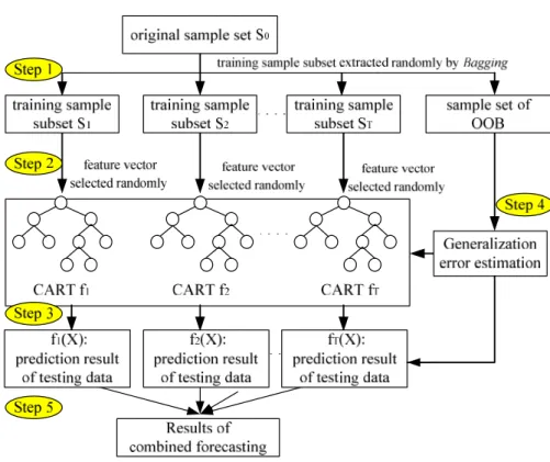
II. BASIC PRINCIPLES OF RANDOM FOREST MODEL
A machine learning technique is an algorithm that estimates the unknown mapping between its inputs and outputs from the observed data. As a theoretical extension of a decision tree, the random forest is a kind of ensemble learning method of the classification and regression tree (CART), and has been applied in fields such as biological information, medical research, business management and text classification [23]. By combining the bagging method and the random subspace theory, the basic principle of RF is to obtain all the decision trees by paralleled training of the sample subsets, re-sample the training samples and their feature
variables randomly, then finally optimize and combine the analysis results of each tree. The flow of the RF model is shown in Fig.1:
Fig. 1. Flow chart of the RF model
Step 1: In the bagging method, suppose the training sample is x, which is affiliated to the sample subsets
i
S . The sample subsets Siare drawn randomly from the original sample set
S
0 with replacement, fromwhich each decision tree is formed, respectively. If the size of the training sample subset is N, the probability
that each sample is not selected can be calculated by Eq. (1) [23]
lim(1 1)N 1 0.368 i N P x x S N e (1)Eq. (1) shows that nearly one-third of the original cases are left out of the training sample. The out-of-bag (OOB) samples can be used to get a running unbiased estimation of the generalization error.
Step 2: Based on the random subspace theory, some feature variables are selected randomly from the training samples to help form the decision tree, so that it grows from root to leaf and reaches the expected
size. Assuming that the number of characteristic variables is m, the node splitting process of each decision
tree is 2m.The Gini coefficient and the maximum information gain principles are adopted to obtain the
variable importance measure (VIM).
Step 3: All these decision trees constitute the random forest. The ensemble learning theory requires that the prediction error of each tree should be less than 50%, so that none of the trees need pruning to ensure the training speed of the model.
Step 4: The unbiased estimation of the generalization error of the RF model is carried out using OOB samples [21]. Due to randomness, the prediction performance of one single decision tree is not stable and its generalization error may be large, but as the number of decision trees increases, the generalization error of the RF will decrease gradually, and finally to a stable limit.
Step 5: The RF model is used to test the sample set, and the combined forecasting results of multiple decision trees are the prediction values of the RF model.
According to ensemble learning theory, double randomness is introduced into the RF methodology by randomly training sampling with replacement using the bagging method, and by randomly extracting specific factors (variables) to participate in training each tree, so that the independence and diversity of the decision trees can be guaranteed. It is not only conducive to improving computational efficiency by parallel training each decision tree, but also to improving the robustness to unknown samples and abnormal data, and furthermore to reducing random error. However, the randomness makes the random forest method like a black box model, and its internal process is difficult to control, resulting in poor interpretability [24]. Its credibility needs to be evaluated by VIM index and OOB errors[25].
Since the OOB samples obey the same distribution as the training sample set, it is difficult to reflect the variation of the forecasting sample set. Therefore, some additional samples need to be added to verify the generalization ability by the external validation index[26].
III. A SUPERVISED RANDOM FOREST FORECASTING MODEL
Based on two-stage feature selection and the supervised random forest (RF), a new model of short-term wind power forecasting is presented in this paper, as shown in Fig.2.
Subset S2 Subset S1 CART fM CART f2 Preformance evaluation of each tree tempera ture 10m wind speed 100m wind speed 70m wind speed Wind power wind direction humidity air pressure … wind power wind speed … … … … V P P365 P1 V1 V365 … Pd10 Pd1 … Vd1 Vd10 … CART f2 Subset SM decision -trees recombin -ation …
(1)two-stage feature selection
Eliminating redundant
features
(2)supervised random forest model
sampling randomly features randomly external validation by NWP reference mRMR Model training Eliminating irrelevant samples Subagging
VIM index correlation coefficient
training sample sets S0 predicting sample sets S1 Intimate samples selection Daily samples separation The key features selection Sample testing
Fig.2 The framework of short-term wind power forecasting model proposed in this paper
(1) The feature selection contains two stages. First, the key features are selected from the historical data sources by the VIM index, such as air temperature, air pressure, wind speed, wind direction and other meteorological data measured at the tower, and historical data of wind power at the wind farms, and then the stream data of those features are converted to daily samples. Second, the intimate samples are identified whose correlation index is strongly related to training and forecasting targets reference by wind speed feom NWP, making the input and output of the forecasting model satisfy the principle of minimal- redundancy &
maximal-relevance (mRMR) [27,28].
(2) The supervised RF is improved to overcome the shortcoming that the OOB error is only adapted to verify the internal training sample set. Based on the idea of transfer learning [29], an external test index considering numeric weather prediction is proposed to evaluate the forecasting performance of each decision tree. Since decision trees that can satisfy merits are allowed to formulate the random forest, the RF of this type is called the supervised random forest.
3.1 Feature selection considering feature importance assessment
Although the time-scale in short-term wind power forecasting is only 1-3 days and there are hundreds of data points (assuming a sampling interval is 15 minutes), the time scale for historical data of each physical variable (including temperature, air pressure, humidity, wind direction, wind speed at different heights and output power of wind farms) is at least a year with nearly 40 thousand data points [30]. In the massive historical data chains with multiple variables, only a few characteristic variables and one part of the data samples are strongly related to the forecasting day. The matrix of characteristics correlation between the forecasting and historical samples is sparse and can hardly meet the mRMR principles. To eliminate the adverse effects of redundant features and unrelated samples, two stages are contained in the data preprocessing link.
3.1.1 Stage one: key feature selection using variable importance measure (VIM)
Using the VIM index, the importance of 10 feature variables is evaluated, including air temperature, air pressure, humidity, wind direction and 10m wind speed, 30m wind speed, 50m hub wind speed, 70m wind speed, 100m wind speed and historical wind power . Only key features remain for the following RF model, which is constructed by 50 decision trees. There are two methods for evaluating the importance of the 10 feature variables.
In method 1, the features are evaluated by the VIM index based on the Gini coefficient principle, as seen in Fig.3 (upper). Only those of the seventh and tenth variables, 50m hub wind speed and historical wind power, are larger than the average (i.e., the dotted line), and the other variables will be irrelevant.
In method 2, the features are evaluated by OOB errors. If each feature is used to train the RF model in turn, the 10 curves of the generalization error are shown in Fig.3(lower). Again, it is found that the generalization errors of two key features, such as 50m hub wind speed and historical wind power, are the lowest, where the conclusion is consistent with that of the VIM index.
The generalization ability of the model before and after feature selection are estimated by OOB error[31]. In order to verify the above conclusions, all 10 features and the two key features are input variables to train the RF model, respectively. As shown in Fig.4, the forecasting errors of training models before and after feature selection are almost the same on different days, but the training cost has decreased significantly, and the average value has decreased from 90.9s to 20.6s. This indicates that the training efficiency of the model can be greatly improved by the key feature selection.
1 2 3 4 5 6 7 8 9 10 0 0.02 0.04 0.06 0.08 0.1
serial number of feature variables
V IM in de x ba se d on g in i c oe ffi ci e nt Temperature 10m w ind speed 30m w ind speed 50m hub w ind speed 70m w ind speed 100m w ind speed w ind direction
w ind pow er output
Humidity Pressures
criteria by the average
Fig.3 Comparison of characteristic importance by different evaluation criteria (a) The VIM index of each variable
0 5 10 15 20 25 30 35 40 45 50
10-2 100 102
number of decision tree
G en er al iz at io n e rr o r / m se Temperature Pressures Humidity w ind direction w ind speed at 10m w ind speed at 30m w ind speed at 50m w ind speed at 70m w ind speed at 100m w ind pow er output criteria by the average
Fig.3 Comparison of characteristic importance by different evaluation criteria (b) the OOB error estimation for each variable 1 2 3 4 5 6 7 8 9 10 0 0.02 0.04 0.06 0.08 0.1 dates pr ed ic tin g er ro r / m se 1 2 3 4 5 6 7 8 9 10 0 20 40 60 80 100 dates tr ai ni ng c os t / s
RF by all the features RF by the key features RF by all the features
RF by the key features
Fig.4 The effect of feature selection on the training of the RF model (left) Forecasting errors between all the variables and key variables (right) Training cost between all the variables and key variables
3.1.2 Stage two: intimate sample identification based on correlation assessment
The daily samples related to prediction (referred to as the ‘intimate samples’) are identified from the massive historical data of the key features, as shown in Fig.5.
short-term wind power forecasting requirements. The correlation degree with reference to the forecasting day is calculated, and then samples are arranged in descending order.
Only 2Mintimate samples
V Vd1, d2,...,VM
P Pd1, d2,...,PM
are identified as the input sample set of the RFmodel (M=10). Several correlation indices are optional[32]. In this paper, the entropy correlation index is adopted. Details can be found in [33,34].
Suppose that the variables areX、 ,Y then the information entropyH and mutual informationI(X;Y)
can be used to quantify the nonlinear mapping relationship between the input and output variables of the prediction model. 2 1 ( ) N ( ) log ( ( ))i i i H X p X p X
(2) ) , ( ) ( ) ( ) ; (X Y H X H Y H X Y I (3)The entropy correlation index is defined as follows:
) ( ) ( ) ; ( Y H X H Y X I IXY (4) As the correlation between the whole original sample set (daily rated power / p.u.) and training target will be very poor. There are a large number of irrelevant samples. Using the correlation evaluation index, some intimate samples are selected that are strongly related to the training objectives, and the regularity of the training samples is more obvious.
Before prediction, a wind speed curve after normalization provided by numerical weather prediction (NWP) is used to match the intimate sample set, instead of the unknown power curve. The wind speed from NWP also has another merit: it contains information from meteorological models (indeed, physical models) that’s suitable for daily-ahead prediction.
The forecasting error and training costs of all samples and intimate samples are shown in Fig.5. It can be seen that after the intimate sample selection, the forecasting error MSE has been reduced for every forecasting day. The average value has decreased from 0.076 to 0.046, and the training cost has also been reduced to less than 0.4 seconds.
1 2 3 4 5 6 7 8 9 10 0 0.02 0.04 0.06 0.08 0.1 0.12 0.14 dates pr ed ic tin g er ro r / m se 1 2 3 4 5 6 7 8 9 10 0 0.5 1 1.5 2 2.5 3 dates tr ai ni ng c os t / s RF by all samples RF by intimate samples RF by all samples RF by intimate samples
Fig.5 Wind power forecasting error and training cost before and after sample screening (left) Original sample set and training target (right) Close sample set strongly related to the training target
3.2 Supervised random forest based on decision tree reorganization
3.2.1 Sampling strategy on generalization error using the subagging method
The bagging method, also called self-aggregation, randomly samples with replacement, and is widely used in the ensemble learning theory. It is equivalent to reconstruct the training sample set[35] obeying the same probability distribution, so that the curve clusters of the intimate samples can be expanded.
Random sub-sampling algorithms, such as the subagging method, can be derived from the bagging method
[36,37]. Assuming that the sampling ratio of training sample sets is n, when n decreases from 1 to 0.1 (n=1
refers to the bagging method, and n<1 refers to the subagging method), the RF model with 50 decision trees is trained successively. The generalization ability is estimated by the OOB error, as shown in Fig 6.
0 10 20 30 40 50 0 2 4 6 8
Number of decision trees
O O B e rr or / m se 0 10 20 30 40 50 10-2 10-1 100 101
Number of decision trees
O O B e rr or / m se n=1.0 n=0.9 n=0.8 n=0.7 n=0.6 n=0.5 n=0.4 n=0.3 n=0.2 n=0.1 Generalization error of RF Generalization error of RF
Fig.6 Effect on generalization error by different sampling ratios (left) Generalization error by different sampling ratios (right) Amplification of generalization error
Seen from Fig.6 (left), with the number of decision-trees increasing, the curves of the generalization error
in the RF model decrease quickly, and then tend to a relatively stable lower limit(mse=104). However, with
n smaller, the curves of the generalization error decrease faster, and the convergence of the training model is
becoming faster, which shows that the subagging method is conducive to improving computational efficiency of the RF model. The generalization error curves are amplified near the lower-limit in the
logarithmic coordinates, as is shown in Fig.6 (right). When n ≥0.5, the lower limits of the generalization
error are almost at the same level, but the limits are relatively larger when n<0.5, which shows that it is
suitable for the RF model when the sampling rate of n is about 0.6. The subagging method, rather than the
bagging method, is proposed in Fig.2.
The effects on the generalization error with respect to different sampling proportions are shown in Fig.7. The training sample set consists of 20 rows and 96 rows of matrices, in which each row represents a data sample of one day, and each column represents data of all sample days at the same time. All rows and all
columns of the matrix are sampled by subagging. The subN model represents random sampling applied on
lines; the subV model represents random sampling applied on columns; and the subNV model represents
sampling applied on all lines and columns.
In Fig.7 (left), as the proportion of sampling increases, the forecasting error of the subN model decreases first and then increases slightly, the subV model has little change, and the subNV model first descends then rises, where the inflection point occurs when the sampling ratio is 50%. With the increase of sampling proportion in Fig.7 (right), the training cost of three models increases. The training cost of the subNV model increases the most, which indicates that the smaller the sampling proportion is, the higher the efficiency of model training is.
10% 20% 30% 40% 50% 60% 0.04 0.045 0.05 0.055 0.06
Sampling ratios of Subagging
pr ed ic tin g er ro r / m se 10% 20% 30% 40% 50% 60% 0.29 0.3 0.31 0.32 0.33 0.34
Sampling ratios of Subagging
tr ai ni ng c os t / s subN subV subNV subN sunV subNV
Fig.7 Effect on generalization error by sample subset corresponding to different sampling proportions (left) Forecasting error (right) Training cost
From the effects on the generalization error with respect to different sampling modes, it can be seen that, compared with the original RF model, the forecasting error and training cost of the subN, subV and subNV models can be reduced, and the improvement of the subN and subNV models are more obvious.
3.2.2 Decision trees reorganization based on the external validation index
The irreverent samples will inevitably be reconstructed from training samples by the bagging method. As a result, some of the decision trees will benefit the later prediction process, while others will not. It is suggested that decision tree reorganization should be added to the RF process (as shown in Fig.2), in which those trees with poor performance are eliminated.
The evaluation index of the decision tree is essential. OOB error is an unbiased estimate of generalization ability in RF models[23], but it only estimates the generalization error of training samples. It is likely to be invalid to estimate the generalization error of forecasting samples, due to the great differences between the forecasting and training samples in short-term wind power forecasting.
Forecasting is the use of limited historical data for model training and the application of knowledge learned in new environments and new tasks. Based on the idea of transfer learning, it is hoped that the features between the source and target domains are as similar as possible[29]. An external validation index based on NWP wind speed, called the relevance index, is proposed in this paper. The relevance index is in fact the Spearman’s rank correlation of samples. Compared with Pearson's correlation coefficient, Spearman's rank correlation coefficient is more appropriate where there is a nonlinear relationship between the forecasting results of each decision tree and the NWP wind speed. The new random forest is reformed by the decision trees that are strongly related to the wind speed of NWP.
The rationality of the above proposal is verified by simulation, as shown in Fig.8 (left.1). The relevance index of the decision trees ranges from 0.04 to 0.07. If the RF model directly composes all the decision trees, the generalization error tends to 0.025 in Fig.8 (right. 1), which is numerical unstable. To solve the problems, it is suggested that all decision trees are arranged in ascending order by the relevance index in Fig.8 (left. 2), and then a new RF model is restructured, with generalization errors as shown in Fig.8 (right.2). Comparatively, the generalization error can quickly decline to 0.005, and then rise up to 0.025 with the addition of some trees that are of poor performance. Thus the generalization error of the RF model decreases not only with more trees, but is also more closely related to relevance index.
Therefore, the post evaluation of the decision trees that have been sorted and reorganized is suggested. The decision trees with a high correlation coefficient are selected in the later prediction. The generalization error of the RF mode is minimum at the inflection point in Fig. 8 (right.2), which indicates the optimal number of decision trees. Considering that the number should not be too small to avoid numerical instability, it is suggested that the decision trees with a better relevance index than the average are selected, as shown in
Fig.8 (left.3). The first 50 decision trees are used in combination in the new RF model. This way, the generalization error is obviously reduced, as shown in Fig.8 (right. 3).
0 20 40 60 80 100
0 0.5 1
Serial numberr of each tree
R el ev an ce in de x 0 20 40 60 80 100 0 0.02 0.04 0.06 0.08
Number of decision trees in RF model
G en er al iz at io n er ro r ( M S E ) ( M S E ) numerical instability 100 80 60 40 20 0 0 0.5 1
Serial numberr of each tree
R el ev an ce in de x 20 40 60 80 100 0 0.02 0.04 0.06 0.08
Number of decision trees in RF model
G en er al iz at io n er ro r ( M S E ) ( M S E ) inflection point average
the first 50 decision trees
0 20 40 60 80 100
0 0.5 1
Serial numberr of each tree
R el ev a nc e in de x 20 40 60 80 100 0 0.02 0.04 0.06 0.08
Number of decision trees in RF model
G en er al iz at io n er ro r ( M S E ) original RF model the RF after decision trees reorganization average
Fig.8 Effect on generalization error of RF model by relevance index of each decision-tree (left) Selection by better relevance index than average (right) Improved RF based on decision-trees reorganization
From the effect of the tree selections via different validation methods in RF model calculated 100 times, it can been seen that, the modified RF models are screened by the OOB error index and by the external validation index are better than the original RF mode in aspect of the forecasting errors and training costs, especially by the external validation index, the forecasting error is reduced significantly.
IV. CASE STUDY OF IMPROVED RF MODE ON APPLICATION
In order to test the feasibility of the supervised RF model, the measured data from a wind farm (installed
capacity SN=49.5MW) in Jilin Province, China, have been used as an example. In the example, historical data
on wind power and meteorological data measured by a wind tower, plus NWP data in the range of 5km for all 12 months in 2015, have been collected. The sampling interval of all data was 15 minutes. These original data are divided into two sample sets: the training sample set proposed by Jan-Nov data, and the test samples set by the data in December. The time scale in short-term wind power prediction is 96 data-points a day (15min per point) and the generalization ability of each prediction model is tested using the monthly average value of the daily MSE indices.
The improved RF model will be compared with the original RF, BP neural network and Support Vector Machine(SVM) from three aspects of performance: the generalization error, computation efficiency and model robustness [38].The main parameters of the model are as follows:
1) The number of decision trees in the improved RF model is set to 50.
2) The number of the hidden-layer nodes is set to 50, and the training algorithm of the BP neural network is L-M optimization (Levenberg-Marquardt), while one of Bayesian neural networks is Bayesian regulation.
3) The kernel function of the SVM is the radial basis function(RBF), whose penalty parameter is C=1. The parameters of the above models are set, in reference to the typical function from the MATLAB R2013b.
4.1 Generalization ability analysis
By comparison of the training error and the prediction error of daily data, it can be seen that, the fitting effect of the training data by the BP neural network model is the best but its prediction result of the testing data is the worst as it is over fitting on the model-training phase, due to the ERM principle. If model-training is appropriately magnified by the SRM principle, the prediction error of the test data will decrease, which implies the generalization ability will be enhanced.
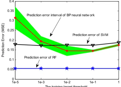
In addition, several calculations show that the numerical stability of the prediction results using the neural network model is rather poor, and the uncertainty of the prediction results is large as a result of random initialization of network parameters (i.e. connection weights and thresholds). To quantitatively analyze the above conclusions, the maximum fitting error of the model training (that is, training target threshold) varies
from 10-5 to 1, and the corresponding prediction errors using the neural network, SVM and RF models are
shown in Fig. 9.
As can be seen in Fig.9, with the training target threshold increasing, the prediction error of the BP neural network decreases first and then increases, and the error band that stems from numerical instability tends to
narrow. Therefore, the threshold of the training target is proposed as 10-2 at the turning point of the error band
in Fig.9, and the average of the prediction results is obtained to eliminate numerical instability by cross validation.
1e-50 1e-3 1e-2 1e-1 1
0.05 0.1 0.15 0.2 0.25 0.3 0.35 0.4
The training target threshold
P re di c tio n E rr o r (M S E ) Prediction error of RF
Prediction error interval of BP neural netw ork
Prediction error of SVM
Fig 9 Influence on prediction results by training target threshold
Compared with the neural network model, the numerical stability of the SVM and RF models are better, and they are less affected by the threshold of the training target. The reason is that the objective function of SVM in the training stage is the SRM principle, instead of ERM, and the problem of local over-fitting may then be solved. In the RF model, randomly re-sampling and OOB error estimation plays the same role as cross validation. As far as the prediction error is concerned, the prediction error of the RF model is lowest and its generalization ability is stronger than the other models.
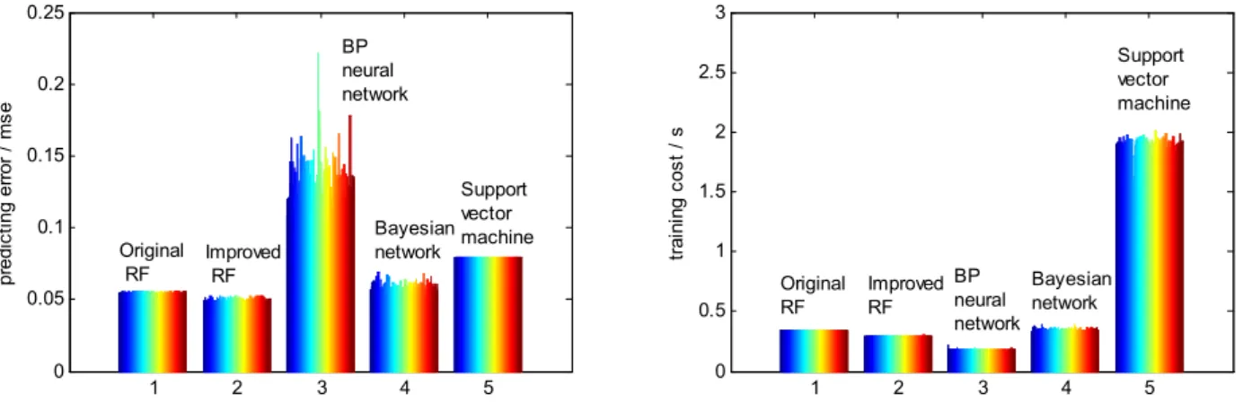
4.2 Comparison of forecasting performance of different models
The forecasting errors and training costs at different dates are calculated by the above five models, as shown in Fig.15. The monthly MSE of daily forecast results is adopted to evaluate the generalization ability of the different models.
is shown in Tab.1. It is shown that the training cost of the BP neural network is the shortest, but its forecasting error is the maximum and its numerical stability is the worst. The forecasting error of the supervised RF model proposed in this paper is the smallest, and relatively stable. The training cost is a little longer, so the advantage is obvious. 1 2 3 4 5 0 0.05 0.1 0.15 0.2 0.25 pr ed ic tin g e rr or / m se 1 2 3 4 5 0 0.5 1 1.5 2 2.5 3 tr ai ni ng c os t / s Improved RF Support vector machine Bayesian network Original RF BP neural network BP neural network Improved RF Original RF Support vector machine Bayesian network
Fig.10 The forecasting error and training cost of five different models calculated at 100 times (left) Forecasting error of different models (right) Training cost of different models
TABLE I COMPARATIVE ANALYSIS OF DIFFERENT MODELS
Different Models The original RF model The improved RF model network modelBP neural network model Bayesian Machine model Support Vector Forecasting error
MSE(%) 0.0548 0.0500 0.1343 0.0597 0.0790
Training cost
(s) 0.3402 0.2972 0.1798 0.3489 1.9008 4.3 Comparison of Noise Robustness
The white noise with a signal noise ratio (SNR)=2%,4%,6%,8%,10% is added to each input and output sample, and the forecasting error and training cost of different modes can be obtained, which is applied to the testing samples set, as shown in Fig.11.
According to Fig.11, the forecasting errors of the 5 models are increased after increasing the white noise with a different SNR. The BP neural network and SVM rank first and second, which indicates that they are sensitive to noise. The training cost of the Bayesian network model is greatly influenced by the noise with the increase of the SNR. The supervised RF model proposed in this paper has the least increase in forecasting error, and the training cost is basically irrelevant to the noise, which is good performance on anti-noise.
2% 4% 6% 8% 10% 2% 4% 6% 8% 0 0.1 0.2 0.3 0.4 0.5 0.6 0.7 SNR pr ed ic tin g er ro r / m se Original RF Improved RF BP neural network Bayesian network Support vector machine
2% 4% 6% 8% 10% 2% 4% 6% 8% 0 0.5 1 1.5 2 SNR tr ai ni ng c os t / s Original RFImproved RF BP neural network Bayesian network Support vector machine
Fig.11 Influence on forecasting results with noise (left) Forecasting error with different SNR (right) Training cost with different SNR
4.4 Robustness of wind power curtailment
Wind power curtailment results in a serious distortion in the historical data. In the paper, the robustness of the forecasting model will be evaluated after the wind power curtailment (setting the value to nearly zero) samples are added. Taking the RF, BP neural network and SVM model, for example, the prediction results are shown in Fig.12. The curtailment happened in the early morning. The original prediction has some nonzero values during the period. Since they does not impact the prediction accuracy evaluation, they are settled to zero for better comparison.
0 20 40 60 80 data points 0 0.5 1 (a)Training data(RF) w in d p ow e r no rm al iz e d Training result True value 0 20 40 60 80 data points 0 0.5 1 (b) Testing data(RF) w in d p ow e r no rm al iz e d Predicting result True value 0 20 40 60 80 data points 0 0.5 1
(a) Training data(BP)
w in d po w er n or m al iz e d Training result True value 0 20 40 60 80 data points 0 0.5 1 (b) Testing data(BP) w in d po w er n or m al iz e d Predicting result True value 0 20 40 60 80 data points 0 0.5 1
(a) Training data(SVM)
w in d po w er n o rm al iz ed Training result True value 0 20 40 60 80 data points 0 0.5 1 (b) Testing data(SVM) w in d po w er n o rm al iz ed Predicting result True value
Fig.12 Distorted data resulting from wind power curtailment of 2 hours in length (upper) using the RF model (middle) using the BP neural network model (lower) using the SVM model
In view of the different beginning time and the different length of the wind power curtailment duration in the historical data, the research on the robustness of the above five forecasting models is discussed.
It is seen from Fig.13 that at different times of wind power curtailment of 2 hours in length, the forecasting error of the SVM and BP neural network is larger and more unstable than the others, and the SVM is the most time-consuming.
It is seen from Fig.14 that with wind power curtailment increasing, the forecasting error of the SVM model and the BP neural network model increases rapidly, and the numerical stability is not good enough. The robustness of the improved RF model proposed in this paper is the best. The reason for this is that the randomly re-sampling of training samples in the RF model is equivalent to reconstructing the original training samples, weakening the dependence on historical samples in the model training. In particular, using the subagging method in a random sampling strategy may reduce the adverse effects of abandoned wind data on the training model, and improve the tolerance to abnormal data in the RF model.
1 2 3 4 5 6 7 8 9 10 0.04 0.06 0.08 0.1 0.12 0.14 0.16 0.18 0.2
wind power curtailment moment / h
pr ed ic tin g er ro r / m se Original RF Improved RF BP neural network Bayesian network Support vector machine
1 2 3 4 5 6 7 8 9 10 0 0.5 1 1.5 2
wind power curtailment moment / h
tr ai ni ng c os t / s Original RF Improved RF BP neural network Bayesian network Support vector machine
Fig.13 The wind power curtailment of 2 hours in length at different times (left) Forecasting error with different times (right) Training cost with different times
0 1 2 3 4 0.05 0.1 0.15 0.2 0.25 0.3 0.35 0.4 0.45
wind power curtailment period / h
pr ed ic tin g er ro r / m se Original RF Improved RF BP neural network Bayesian network Support vector machine
0 1 2 3 4 0 0.5 1 1.5 2
wind power curtailment period / h
tr ai ni ng c os t / s Original RF Improved RF BP neural network Bayesian network Support vector machine
(a) Forecasting error to different extent (b) Training cost to different extent
Fig.14 The duration of wind power curtailment is prolonged by half an hour (left) Forecasting error to different extent (right) Training cost to different extent
V. CONCLUSIONS
To solve the over-fitting problems of the BP neural network in the model-training stage, the RF model rooted in ensemble learning has been applied to short-term wind power forecasting, whose random re-sampling strategy makes the forecasting model more adaptive to the fluctuation and randomness of wind power. However, the RF model still requires some improvement to enhance the interpretability of the black-box model, and a new model of short-term wind power forecasting has been proposed based on two-stage feature selection and a supervised random forest in this paper. The specific conclusions are as follows:
(1)Due to the obvious sparsity of a correlation matrix between the forecasting and historical daily samples, the redundant features and irrelevant samples have been eliminated from the training sample set, in the data pretreatment of two-stage feature selection by VIM index and relevant analysis, and it has been verified that both the model training efficiency and the degree of correlation between input and output samples are improved.
(2) A supervised random forest model based on decision trees’ reorganization has been constructed, in order to improve the interpretability of the original RF model. An external validation index referring to the NWP wind speed, called the relevance index, has been proposed to avoid the defect of the existing OOB error, which still depends on the training samples as the internal validation. The case study shows that the external test index can further enhance the generalization ability of the RF model.
(3) Taking the measured data of a wind farm as an example has proved that, compared with the original RF, BP neural network, Bayesian network and SVM model, the improved RF model has a better effect in aspects of ensuring accuracy, efficiency and robustness, especially if there is high rate of noisy data and wind power curtailment duration in the historical data.
ACKNOWLEDGEMENT
The project is supported by State Grid Corporation technology project “Key Technologies of Operation and Control of Power Systems with High Proportion of Wind Power”.
VI. REFERENCES
1. P Bauer, A Thorpe, G Brunet. The quiet revolution of numerical weather prediction[J]. Nature, 2015, 525:47-55.
2. J Dowell, S Weiss, D Hill, D Infield. Short-term spatio-temporal prediction of wind speed and direction[J]. Wind Energy, 2014,17(12): 1945-1955.
3. J Badger, H Frank, A N Hahmann, G Giebel. Wind-Climate Estimation Based on Mesoscale and Microscale Modeling: Statistical- Dynamical Downscaling for Wind Energy Applications[J]. Journal of Applied Meteorology & Climatology,2014,53(8): 1901-1919.
4. Giebel G, Kariniotakis G. Wind power forecasting-a review of the state of the art,in Renewable Energy Forecasting: From Models to Applications. Kariniotakis G (ed). Woodhead Publishing. 1st edn, 2017: 59-109.
5. ANEMOS.plus. The State-Of-The-Art in Short-Term Prediction of Wind Power: A Literature Overview, 2nd edition. 2011. 6. P Pinson . Wind Energy: Forecasting Challenges for Its Operational Management[J]. Statistics,2013,28(4): 564-585.
7. J Tastu, P Pinson, E Kotwa, H Madsen, H A Nielsen. Spatio-temporal analysis and modeling of short-term wind power forecast errors[J]. Wind Energy, 2011, 14(1): 43-60.
8. B Lange, K Rohrig, et al. Wind power prediction in Germany Recent advances and future challenges[C]. European Wind Energy Conference, Athens, 2006.
9. M Lange, U Focken. New developments in wind energy forecasting[C]. Power & Energy Society General Meeting-conversion & Delivery of Electrical Energy in the Century, 2008:1-8.
10.S A Kalogirou. Artificial neural networks in renewable energy systems applications: a review[J]. Renewable & Sustainable Energy Reviews, 2001,5(4):373-401.
11.Nitish Srivastava, Geo_rey Hinton, Alex Krizhevsky. Dropout: A Simple Way to Prevent Neural Networks from Overfitting[J]. Journal of Machine Learning Research, 2014,15: 1929-1958.
12.W Q Zhao, Y M Wei, Z Y Su. One day ahead wind speed forecasting: A resampling-based approach[J]. Applied Energy, 2016, 178:866-901 13.G X Jiang, W J Wang. Error estimation based on variance analysis of k-fold cross-validation[J]. Pattern Recognition.2017(69):94-106 14.K P Shi, Y Qiao, W Zhao, et al. Study on Short-Term Prediction Considering Entropy Association Information Mining of Historical
Data[J].Automation of Electric Power Systems, 2017,41(3): 13-18.
15.Vapnik V N. An overview of statistical learning theory[J]. IEEE Transactions on Neural Networks,1999,10(5): 988-999. 16.C Cortes, V Vapnik. Support-vector networks[J]. Machine Learning, 1995, 20(3): 273-297.
17.C J Burges. A tutorial on support vector machines for pattern recognition[J]. Data Mininng and Knowledge Discovery, 1998, 2(2):121-167. 18.Vahid Kazemi, Josephine Sullivan. One Millisecond Face Alignment with an Ensemble of Regression Trees[J]. Computer Vision & Pattern
Recognition, 2014: 1867-1874.
19.M R. Segal. Machine Learning Benchmarks and Random Forest Regression[J]. 2003 Kluwer Academic Publishers. Printed in the Netherlands 20.M Fernández-Delgado, E Cernadas, etal. Do we Need Hundreds of Classifiers to Solve Real World Classification Problems?[J] Journal of
Machine Learning Research 2014, 15:3133−3181.
21.F Thordarson, H Madsen, HA Nielsen P Pinson. Conditional weighted combination of wind power forecasts[J]. Wind Energy, 2010, 13(8): 751-763.
22.P Pinson , H Madsen. Ensemble-based probabilistic forecasting at Horns Review[J]. Wind Energy, 2009, 12(2): 137-155. 23.L Breiman. Random Forests[J]. Machine Learning,2001,45(1): 5-32.
24.S.H.Welling, H.F.Refsgaard, P.B.Brockhoff. Forest Floor Visualizations of Random Forests[J]. https://www.researchgate.net/publication /303683745 _Forest_Floor_Visualizations_of_Random_Forests.
25.D H Wolpert, W G Macready. An Efficient Method to Estimate Bagging' s Generalization Error[J] .M achine Learning, 1999,35(1):41-55. 26.L T QIN, S S LIU, QF XIAO, et al. Internal and external validtions of QSAR model: Review[J]. Environmental Chemistry, 2013, 32(7):1205
-1211.
27.YN ZHAO, L YE. A Numerical Weather Prediction Feature Selection Approach Based on Minimal-redundancy- maximal-relevance Strategy for Short-term Regional Wind Power Prediction[J]. Proceedings of the CSEE, 2015,35(23):5985-5994.
28.J X Che, Y L Yang, L Li, et al. Maximum relevance minimum common redundancy feature selection for nonlinear data[J]. Information Sciences, 2017, 409-410:68-86.
29.C.Perlich B. Dalessandro T. Raeder O, et al . Machine learning for targeted display advertising: Transfer Learning in action[J]. Mach Learn, 2014,95:103-127.
30.M Ranaboldo, G Giebel, B Codina. Implementation of a Model Output Statistics based on meteorological variable screening for short-term wind power forecast[J]. Wind Energy. 2013, 16(6): 811-826.
31.H C Peng, F H Long, Chris Ding. Feature selection based on mutual information criteria of max-dependency, max-relevance, and min- redundancy[J]. IEEE Transactions on Pattern Analysis and Machine Intelligence,2005, 27(8): 1226- 1238.
32.Geoffrey M.Henebry. Spatial model error analysis using autocorrelation indices[J]. Ecological Modelling, 1995,82(1): 75-91.
33.KP Shi, Y Qiao, W Zhao, et al. Study on Short-Term Prediction Considering Entropy Association Information Mining of Historical Data[J].Automation of Electric Power Systems, 2017,41(3): 13-18.
34.T S Nielsen, A Joensen, H Madsen, et al. A new reference for wind power forecasting[J]. Wind Energy, 2015, 1(1): 29-34. 35.L Breiman. Bagging predictors[J]. Machine Learning,1996, 24: 123-140.
36.C Zhang, X Bian, P Liu, X Tan, Q Fan. Subagging for the improvement of predictive stability of extreme learning machine for spectral quantitative analysis of complex samples[J]. Chemometrics & Intelligent Laboratory Systems, 2017, 161, 43-48.
37.R Arlindo. F Galvão, R H Roberto, et al. Effect of the subsampling ratio in the application of subagging for multivariate calibration with the successive projections algorithm[J].Journal of the Brazilian Chemical Society, 2011.22(11): 2225-2233.
38. E RENDON, I M. ABUNDEZ, C GUTIERREZ, etal .A comparison of internal and external cluster validation indexes[J]. Applications of Mathematics and Computer Engineering.158-163. http://www.doc88.com/p-171327434946.html.
39.D J Burke, M J O'Malley. Factors Influencing Wind Energy Curtailment[J]. IEEE Transactions on Sustainable Energy, 2011, 2 (2): 185-193. 40.G L Luo,Y L Li, W J Tang, X Wei. Wind curtailment of China׳s wind power operation: Evolution, causes and solutions[J]. Renewable &
Sustainable Energy Reviews, 2016 , 53 :1190-1201. .