Michael Pippig
Massively Parallel,
Fast Fourier Transforms
and Particle-Mesh Methods
Michael Pippig
Massively Parallel,
Fast Fourier Transforms
and Particle-Mesh Methods
Universitätsverlag Chemnitz
2016
Bibliografische Information der Deutschen Nationalbibliothek
Die deutsche Nationalbibliothek verzeichnet diese Publikation in der Deutschen Nationalbibliografie; detaillierte bibliografische Angaben sind im Internet über
http://dnb.d-nb.de abrufbar.
Diese Arbeit wurde von der Fakultät für Mathematik der Technischen Universität Chemnitz als Dissertation zur Erlangung des akademischen Grades
Dr. rer. nat. genehmigt.
Die Arbeit wurde in englischer Sprache verfasst.
Tag der Einreichung: 25. Juni 2015
Betreuer: Prof. Dr. Daniel Potts, Technische Universität Chemnitz 1. Gutachter: Prof. Dr. Daniel Potts, Technische Universität Chemnitz 2. Gutachter: Prof. Dr. Christian Holm, Universität Stuttgart
3. Gutachter: Prof. Dr. Matthias Bolten, Universität Kassel Tag der öffentlichen Prüfung: 13. Oktober 2015
Technische Universität Chemnitz/Universitätsbibiliothek
Universitätsverlag Chemnitz
09107 Chemnitz
http://www.tu-chemnitz.de/ub/univerlag
Herstellung und Auslieferung
Verlagshaus Monsenstein und Vannerdat OHG Am Hawerkamp 31
48155 Münster
http://www.mv-verlag.de
ISBN 978–3–944640–76–1
Contents
1 Introduction 9
2 Parallel fast Fourier transforms 17
2.1 Definitions . . . 20
2.2 One-dimensional fast Fourier transforms . . . 21
2.2.1 Pruned fast Fourier transform . . . 21
2.2.2 Fast Fourier transform with shifted index sets . . . 22
2.2.3 Pruned fast Fourier transform with shifted index sets . . . 23
2.3 Multidimensional fast Fourier transform . . . 24
2.4 Basic modules for multidimensional array transformation . . . 27
2.4.1 The serial FFT module . . . 28
2.4.2 The local transposition module . . . 29
2.4.3 Combination of serial FFT and local transposition . . . 29
2.4.4 Parallel block decomposition . . . 30
2.4.5 Folding multidimensional arrays in row-major order . . . 31
2.4.6 Parallel matrix transposition . . . 32
2.4.7 The parallel multidimensional transposition module . . . 34
2.5 Parallel FFT with multidimensional data decomposition . . . 35
2.6 Parallel pruned FFT . . . 40
2.7 Parallel FFT with shifted index sets . . . 42
2.8 The ghost cell communication modules . . . 44
2.9 The PFFT software library . . . 46
2.10 Numerical results . . . 48
2.10.1 Description of the parallel computing architectures . . . 48
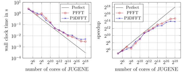
2.10.2 Strong scaling behavior of PFFT on JUGENE . . . 48
2.10.3 Comparison of PFFT and FFTW on JUROPA . . . 49
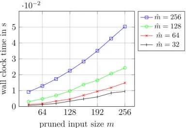
2.10.4 Parallel pruned FFT on JUGENE . . . 49
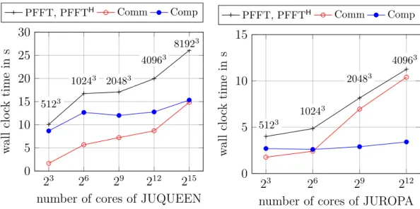
2.10.5 Weak scaling behavior of PFFT on JUQUEEN and JUROPA 50 2.10.6 Strong scaling behavior of PFFT on JUQUEEN and JUROPA 51 3 Parallel nonequispaced fast Fourier transforms 55 3.1 Definitions . . . 56
3.2 The three-dimensional NFFT algorithm . . . 57
3.2.4 Optimized deconvolution . . . 69
3.3 The parallel three-dimensional NFFT . . . 74
3.3.1 Parallel data decomposition . . . 74
3.3.2 Description of the algorithm . . . 74
3.4 The parallel three-dimensional NDFT . . . 81
3.5 The PNFFT software library . . . 81
3.6 Numerical results . . . 83
3.6.1 Strong scaling of pruned PNFFT on JUGENE . . . 84
4 Parallel particle-mesh methods based on NFFT 89 4.1 Definitions . . . 90
4.2 The Ewald splitting . . . 92
4.3 The short-range and self interaction modules . . . 94
4.4 The long-range interaction module . . . 96
4.4.1 The common approximation framework and fast algorithm . . 96
4.4.2 Periodicity in three dimensions . . . 97
4.4.3 Periodicity in two dimensions . . . 99
4.4.4 Periodicity in one dimension . . . 101
4.4.5 Periodicity in no dimension . . . 102
4.4.6 Two-point Taylor interpolation using Newton basis polynomials103 4.4.7 Some notes on Fourier approximations of non-periodic functions105 4.5 The P2NFFT framework . . . 109
4.6 The relation of P2NFFT and P3M . . . 109
4.6.1 Interlaced P2NFFT and P3M . . . 113
4.7 The relation of P2NFFT to other particle-mesh methods . . . 116
4.7.1 Fast summation with non-periodic boundary conditions . . . . 117
4.7.2 Ewald summation . . . 118
4.7.3 Fast Ewald summation based on NFFT . . . 119
4.7.4 Particle-mesh Ewald . . . 119
4.7.5 Smooth particle-mesh Ewald . . . 119
4.7.6 Gaussian split Ewald . . . 120
4.7.7 Spectrally accurate Ewald . . . 120
4.8 Complexity of Ewald summation and parameter selection . . . 120
4.8.1 Runtime model . . . 123
4.8.2 Potential computation via Ewald summation . . . 124
4.8.3 Potential computation via P2NFFT . . . 124
4.8.4 Field computation via Ewald summation . . . 125
4.8.5 Field compuation via P2NFFT . . . 127
4.8.6 Selection of P2NFFT parameters . . . 127
7 4.10 The parallel P2NFFT software library . . . 134
4.11 Numerical results . . . 135 4.11.1 Description of test systems . . . 135 4.11.2 Parameter selection and accuracy of 3d-periodic P2NFFT . . . 136
4.11.3 Parameter selection and accuracy for mixed periodicity . . . . 137 4.11.4 Strong scaling of 0d-periodic P2NFFT on JUGENE . . . 138
4.11.5 Comparison of P2NFFT to other fast Coulomb solvers . . . . 141
List of publications 147
Bibliography 149
List of algorithms 157
1 Introduction
The development of efficient numerical algorithms can, without exaggeration, be called the fundamental basis of high performance computing. For sure, the perma-nent increase of computing power has changed our life in many ways. Problems that have been considered practically not computable for many years are now solv-able within seconds. However, this enormous speedup would not have been possible without the development of adapted algorithms that are able to exploit the available computing power. Thereby, the continual change of computing architectures poses great challenges to the design of sustainable high performance software and requires repeated algorithmic rethinking.
The current trend of hardware design is mainly driven by massive parallelism. This includes shared memory parallelism, distributed memory parallelism, paral-lelism due to accelerators such as graphics processing units, and also any combi-nation of these three. Still, programmers also have to consider the more or less traditional performance relevant problems such as optimal cache utilization and in-struction set extensions like SSE and AVX - just to name a few. Programming on these environments gets increasingly sophisticated, which emphasizes the need for optimized software packages that encapsulate the solution of sub-problems within standalone modules. Note that typical applications in scientific computing are con-glomerates of many different algorithmic modules. In most cases it is practically impossible to know all the performance relevant details of each algorithmic step. In-stead, we may rely on low-level software modules that are highly optimized for these specific tasks. The philosophy behind this thesis is to reuse such low-level modules as much as possible and combine them to higher-level modules. The benefits of this so-called modularized approach are obvious. First of all, the modularized view on algorithms reveals a lot of common structure that simplifies programming and prevents code repetition. Second, improvements of low-level modules automatically inherit to higher-level modules, i.e., performance optimization can be focused on the modular level.
One can think of several attributes that such a software module should have as minimal requirements. Obviously, this list will strongly depend on the precise application of the software but we give a non-exhaustive list of important features that stand in the focus the present thesis:
• Low complexity: A focus on large problem sizes emphasizes the impact of fast algorithms. Within this thesis fast means that an algorithm scales almost linear in the number of degrees of freedom N, i.e., the number of arithmetic
operations increases at most proportional toNlogN.
• Hardware adaptivity: A software module should be portable to a broad vari-ety of hardware architectures and result in high performance on all of these architectures.
• Parallel scalability: In order to exploit the computing power of massively par-allel architectures, all software modules should be scalable in terms of runtime and memory consumption. This implies that the underlying algorithms must be adapted in order to circumvent scalability bottlenecks. Within this the-sis we aim for distributed memory parallelism for hundreds of thousands of processes.
• Error control and parameter selection: Approximate algorithms often intro-duce a set of parameters that can be used to balance the required accuracy against the total computation time. In this case precise error estimates are desirable in order to assist selection of optimal parameters.
• Flexibility: The design of our algorithms should be abstract enough in order to suit a broad variety of applications. Optimizations that only effect rare use cases should not end up in a completely new software module.
• Usability: The sophisticated optimizations and algorithmic details should be hidden from the user by an easy to use interface.
• Public availability: All modules should be available as part of open source software libraries that are freely available. This makes it possible for other researchers to compare the underlying algorithms and contribute to the devel-opment process.
To find the modular structure of algorithms can not always be assumed to be trivial. Indeed, the use of different viewpoints and notation often leads to inde-pendent reinvention of algorithms in scientific literature. Also approaches that look remarkably different at the first sight may turn out to be closely related from an appropriate viewpoint. This is especially true for the broad variety of publications about the Fast Fourier Transform (FFT). In [127] the rigorous use of matrix-vector notation led to an unified framework that reveals the common structure and hid-den beauty of supposedly distinct FFT approaches. The structured view not only helped to understand and classify existing FFT algorithms but also resulted in the discovery of new approaches. On the one hand, the vast variety of different FFT approaches makes it hard to choose the best suitable algorithm for a given problem; on the other hand, plurality gives the chance of algorithmic adaption with respect to changing hardware. A very elegant exploitation of this fact defines the design concept of the FFTW [57, 58] software library. Under the hood FFTW takes into account many different highly optimized FFT approaches and chooses the fastest one at runtime. However, the sophisticated implementation is hidden from the user by an easy to use interface. In this sense, FFTW fulfills all of the above mentioned criteria of a software module but one, namely, high scalability on distributed mem-ory architectures. This led to the development of PFFT – an extension of FFTW
1 Introduction 11
to massively parallel architectures that will be the topic of Chapter 2 in this thesis. Another example that stands in the focus of this thesis is given by the diverse literature about particle-mesh methods. These are fast numerical methods for com-puting the Coulomb interactions between N charged particles in three-dimensional space. Loosely speaking, the basic concept of particle-mesh methods is to convert the given data in a suitable way such that fast Fourier transforms can be applied. Thereby, it is necessary to pre-process and post-processes the data in order to con-nect the irregularly distributed particle positions with the equispaced mesh points of the FFT. Within Chapter 4 of this thesis we show that so-called nonequispaced Fourier transforms (NFFTs) represent a powerful tool to reveal the common modu-larized structure of particle-mesh methods. NFFTs are generalizations of the FFT to nonequispaced sampling points and have been studied and optimized for a long time. Based on the NFFT framework we are able to summarize all particle-mesh methods within one unified framework called Particle-Particle–NFFT (P2NFFT).
However, before this unified picture can be drawn, it is necessary to extend the NFFT framework by several algorithmic modules that are motivated by particle-mesh methods but also recur in other applications of NFFT. This will be the main topic of Chapter 3 of this thesis. We will see that the modularized view of particle-mesh algorithms in terms of NFFTs leads to novel algorithmic developments of both – NFFT and particle-mesh methods.
To this end, the present thesis is about three algorithmic frameworks that are built on top of each other, namely FFT→NFFT→P2NFFT. Each of these frameworks is
designed with the above listed software module requirements in mind. Special em-phasis will be placed on the parallel scalability on distributed memory architectures up to hundreds of thousands of processes. More precisely, this thesis is structured in the following three parts that are devoted to the three self-contained frameworks.
Outline of the Thesis
Chapter 2: Parallel fast Fourier transforms
At first, we derive the PFFT Framework2.5 – a highly scalable FFT framework de-signed for massive parallelism on distributed memory architectures. We start with some elementary definitions in Section 2.1. In Sections 2.2 and 2.3 we introduce the concept of pruned FFT with possibly shifted index sets in one and multiple dimensions. These FFT adaptions appear naturally during the approximation of non-periodic functions by finite Fourier series and will be an important ingredient of the algorithmic frameworks presented in the following chapters. We derive var-ious representations of pruned FFT and FFT with shifted index sets in order to have the freedom to choose the most scalable approach for parallelization later on. As an interim result we get Corollary 2.3 that shows how one-dimensional pruned
FFT with shifted index sets can be computed without explicit data shifts. The multidimensional generalization of this fact is given in (2.9).
Next, in Section 2.4 we show how the algorithms that are already implemented within the FFTW software library can be turned into two powerful algorithmic modules for operating on parallel block-decomposed data. More precisely, these are the serial FFT and transposition module presented in Section 2.4.3 and the parallel multidimensional transposition module introduced in Section 2.4.7. Special attention is given to the generality of these modules. Especially, the pitfalls of unequal block decomposition in multiple dimensions are investigated in detail in Section 2.4.5.
We will see that the above mentioned two modules are sufficient to derive the main result of this chapter – the versatile PFFT Framework 2.5 for computing massively parallel FFT in a highly scalable way. Furthermore, we present the PFFTH Framework 2.6 that essentially computes the parallel inverse FFT.
In Sections 2.6 and 2.7 we compare the different approaches for computing pruned FFT and FFT with shifted index sets with respect to their parallel scalability. It turns out that the most scalable approach is to apply pruning on a per-dimension basis, while shifted index sets should be incorporated by a suitable rescaling in Fourier space. Of course, our PFFT Framework 2.5 is based on these most scalable approaches. Furthermore, we give a brief overview of two ghost cell communication modules in Section 2.8. These modules accomplish the frequently occurring task of next neighbor communication in distributed memory parallelism.
As a major result of this chapter, a freely available implementation of PFFT is presented in Section 2.9. This exceptionally flexible software module is not only basis for all of the following frameworks in Chapters 3 and 4 but also deserves appreciation as a standalone library. Finally, we provide numerical evidence for the high scalability of our parallel FFT implementation with an extensive list of numerical tests in Section 2.10. These tests include investigation of strong and weak scaling on multiple hardware architectures as well as performance evaluations of parallel pruned FFT.
Parts of this chapter have already been published in condensed form in the peer-reviewed papers [4, 2]. A self-contained software library based on the PFFT frame-work is freely available at [11]. Most of the performance measurements have been published as parts of the proceedings [9, 7, 8].
Chapter 3: Parallel nonequispaced fast Fourier transforms
The second framework presented in this work is PNFFT – a highly scalable NFFT framework designed for massive parallelism on distributed memory architectures. It makes use of the previously derived PFFT framework from Chapter 2 but also incorporates many other algorithmic modules that are presented in this chapter.
1 Introduction 13
NFFT approximation ideas at the beginning of Section 3.2. Hereby, we introduce the new concept of pruned NFFT that can be understood as the nonequispaced analog of pruned FFT and becomes important for the evaluation of non-periodic Fourier approximations. Furthermore, we present two fast approaches for the computation of the NFFT’s gradient that originate from particle-mesh methods but have never been considered as individual modules of the NFFT framework before. In Section 3.2.2 we introduce the new concept of shifted NFFT, i.e., an approximation similar to NFFT but with a mesh shifted by half the inverse mesh size. This enables us to transfer the concepts of interlacing from particle-mesh methods to the NFFT framework in Section 3.2.3. Interlacing can be understood as the average of standard NFFT outputs and shifted NFFT outputs. As far as we know, this is the first time that interlacing is considered in the context of the modularized NFFT framework. Another theoretical result on NFFT is presented in Section 3.2.4. There, we derive the formulas of optimal deconvolution coefficients of all presented NFFT types with respect to a mean square aliasing error. Also the interlaced NFFT is considered and the accuracy improvement of interlacing can be shown analytically. We emphasize that these optimized coefficients yield the missing link between NFFT and P3M – a
special kind of particle-mesh algorithm; cf. Chapter 4 for a detailed comparison of both methods.
In Section 3.3 we derive the PNFFT Framework 3.1 and the PNFFTH Frame-work 3.2 for computing the NFFT and its adjoint in parallel. Thereby, we pay special attention to parallel scalability and make use of the parallel FFT frame-works that have been derived in the previous chapter. The parallel modules for the direct computation of nonequispaced discrete Fourier transforms in Section 3.4 further extend the flexibility of the PNFFT framework and provide the link between PNFFT and Ewald summation later on in Section 4.7.2. A freely available imple-mentation of PNFFT is presented in Section 2.9. Finally, the numerical tests in Section 3.6 proof the high scalability of our parallel NFFT frameworks.
Parts of this chapter are based on the peer-reviewed paper [5]. The PNFFT framework has been published as a self-contained software library called PNFFT, which is freely available at [12]. We emphasize that the PNFFT library is the first open source, massively parallel software library for computing the NFFT.
Chapter 4: Parallel particle-mesh methods based on nonequispaced fast Fourier transforms
The last chapter is devoted to the Particle-Particle–NFFT (P2NFFT) – an
NFFT-based, fast framework for the computation of Coulomb interactions.
After some introductory part we define the Coulomb problem with mixed-periodic boundary conditions in Section 4.1 and review the Ewald splitting – a well know approach for splitting Coulomb interactions into short-range and smooth long-range contributions – in Section 4.2. Afterward, the derivation of an algorithmic module
for the computation of the short-range part is straightforward; see Section 4.3. In Section 4.4 we take a closer look at the smooth long-range part. Thereby, we present a new NFFT-based long-range interaction Module 4.3 for the fast computation of the long-range part in Section 4.4.1. In the following Sections 4.4.2–4.4.5, we show that this module can be applied for all types of periodicity. A crucial point is the correct treatment of non-periodic boundary conditions in order to get highly accurate Fourier approximations at modest mesh sizes. Our approach involves the embedding of non-periodic functions into smooth periodic functions that can be approximated well by finite Fourier series. Thereby, smoothness in the endpoints is ensured by continuation with a special kind of Hermite-Birkhoff interpolation. In Section 4.4.6 we present a new representation of such an interpolating polynomial in terms of Newton basis polynomials that allows an efficient evaluation. A detailed comparison of our continuation approach to other proposed Fourier approximations of non-periodic functions from the literature is given in Section 4.4.7.
Altogether, the modules for computing the short-range and long-range parts are combined in Section 4.5 and form the very flexible P2NFFT Framework 4.4. The
close connection of 3d-periodic P2NFFT and the Particle-Particle–Particle-Mesh
(P3M) method is subject of investigation in Section 4.6. We show that P3M is
essentially a special case of P2NFFT and that NFFTs provide a modularized view
on P3M. A unique characteristic of P3M is its optimal deconvolution in Fourier space
with respect to the mean square aliasing error. Almost the same deconvolution can be derived by P2NFFT with the optimal NFFT deconvolution that was derived in
Section 3.2.4. Furthermore, we show in Section 4.6.1 that application of interlaced NFFT to P2NFFT results in four kinds of interlaced particle-mesh algorithms – only
two of them have been considered in the literature for interlaced P3M. However, we
will also see that we can save one FFT in interlaced P3M if we apply one of the two
new interlacing approaches.
Beside P3M, many other particle-mesh methods are included in the P2NFFT
framework. We review some of them in Section 4.7. These include NFFT-based fast summation, Ewald summation, NFFT-based fast Ewald summation, the Particle-Mesh Ewald method, the Smooth Particle-Particle-Mesh Ewald method, Gaussian Split Ewald and Spectrally Accurate Ewald.
Section 4.8 is devoted to a rigorous investigation of the asymptotic runtime of Ewald summation and P2NFFT. Although it is very popular that Ewald
summa-tion scales as O(N3/2) for optimal choice of parameters, we show that this is only
true for the computation of the Coulomb fields. Indeed, the computation of the Coulomb potential scales slightly worse as O((NlogN)3/2). On the other hand, optimal choice of parameters can turn the P2NFFT into a method that scales as
O(N√logN) for the field computation and as O(N√logN(log logN)3/2) for the potential computation. Note that this is slightly better than the commonly cited
O(NlogN) scaling of particle-mesh methods.
1 Introduction 15
that enables us to tune the 7 available P2NFFT parameters for arbitrary prescribed
root mean square error bounds. Thereby, 2 parameters can be eliminated by error bounds of the real space and Fourier space parts, one parameter can be assumed fixed in order to reach machine precision, 3 parameters have to be tuned for small test systems and can be kept constant with increasingN, and the last free parameter can be tuned in order to balance the real and Fourier space computation times.
The parallel P2NFFT Framework 4.8 introduced in Section 4.9 is a generalization
of P2NFFT to massive parallelism on distributed memory architectures. The main
ingredients are the parallel NFFT frameworks that have been derived in Chapter 3. A parallel implementation of P2NFFT is part of the ScaFaCoS software library and
will be presented in Section 4.10.
Finally, we provide numerical evidence for the validity of the P2NFFT parameter
tuning up to high precision in Section 4.11. Furthermore, we compare P2NFFT to
other fast Coulomb solvers with respect to runtime and parallel scalability.
Parts of this chapter are based on the peer-reviewed papers [5, 1, 3] and the proceedings [6]. A freely available implementation of the P2NFFT framework has
Acknowledgments
During the preparation of this thesis I enjoyed the help of many people. It is not an exaggeration to say, that this work would not have been possible without their support and I express my sincere gratitude to all of them. First of all, I like to thank my wife Jule for the continuous assistance and encouragement. I also thank my son Gustav and the rest of my family for their patience and tolerance regarding my limited free time due to long nights of programming.
I want to proclaim my deep appreciation to Prof. Dr. Daniel Potts – founder of the topic and outstanding adviser for many years. His expertise not only enriched my academic work but also my personality. Furthermore, I gratefully acknowledge the help of Prof. Dr. Christian Holm and Prof. Dr. Matthias Bolten, who agreed to examine this thesis.
A special thanks goes to my colleague Franziska Nestler. Her rigorous mathe-matical understanding really pushed forward the generalization of our particle-mesh methods to mixed-periodic boundary conditions. Beside Franziska I also like to thank all the other members of the working group on Applied Functional Analysis at Technische Universität Chemnitz for the nice atmosphere and fruitful discussions during the coffee breaks.
Many thanks go to all the contributors of the ScaFaCoS project. Especially, I want to acknowledge the great help of the following persons: Dr. Godehard Sutmann always managed to support me with computing time. I really adore him for his broad understanding of particle methods. From Dr. Axel Arnold and Dr. Olaf Lenz I gained a lot of experience on particle-mesh methods and code optimization. The competition with the FMM library authored by Dr. Holger Dachsel and Dr. Ivo Kabadshow initiated many performance improvements in my codes. Dr. Michael Hofmann did an excellent job in the support of massively parallel sorting, short-range interactions and build systems. I seriously admire his fast and helpful responses to my putative bug reports. Rene Halver put a lot of effort into the user friendliness of the ScaFaCoS library and Dr. Franz Gähler enforced invaluable improvements of our software packages due to his endless tests and applications to real world problems. Again, many thanks go to all of them.
This work was partly supported by the German Ministery of Science and Edu-cation (BMBF) under grant 01IH08001. Last but not least, I am grateful to the Jülich Supercomputing Center for providing the computational resources on Jülich Blue Gene/P (JUGENE), Jülich Blue Gene/Q (JUQUEEN) and Jülich Research on Petaflop Architectures (JUROPA).
2 Parallel fast Fourier transforms
Without doubt, the fast Fourier transform (FFT) is one of the most important algorithms in scientific computing. It provides the basis of many fast algorithms and there is no chance to give an exhaustive list of the tremendous number of ap-plications. The crucial point in these applications is that the FFT reduces the complexity from O(N2) to O(NlogN), whereby N denotes the total number of degrees of freedom. For large N this comes with an enormous decrease in runtime. The original FFT algorithm was published in 1965 [32], although it was already known to Gauss [69]. Since then, an immense number of alternative algorithms and generalizations has been published, including FFT algorithms for arbitrary input size N, in-place algorithms, shared and distributed memory parallelism, FFTs on graphics processing units, optimized cache use, and many more hardware specific optimizations. A nice survey and abstract view is provided in [127]. But even this book does not include all the different approaches that have been used to find FFT algorithms. This variety of algorithms and the continuous change of hard-ware architectures made it practically impossible to find one FFT algorithm that is best suitable for all circumstances. This shortcoming led to the development of the FFTW [57] software library. Under the hood, FFTW compares a wide variety of different FFT algorithms and measures their runtime to find the most appro-priate one for a given problem size and hardware architecture. The sophisticated implementation is hidden behind an easy interface structure. Therefore, users of FFTW are able to apply highly optimized FFT algorithms without knowing all the details about them. These algorithms have been continuously improved by many collaborators in order to support new hardware trends, such as SSE, AVX, graphics processing units, shared memory parallelism, distributed memory parallelism and so on.
Since the focus of this chapter is distributed memory parallelism for multidimen-sional FFTs we take a closer look at the available algorithms. There are two main approaches; the first is binary exchange algorithms, and the second is transpose algo-rithms. An introduction and theoretical comparison can be found in [66]. However, the second approach has been used in most implementations since it allows the use of highly optimized serial FFT kernels and offers a lot of flexibility. For a closer look at this approach we assume a three-dimensional input array of size ˆm0×mˆ1×mˆ2 with
ˆ
m0 ≥mˆ1 ≥mˆ2. For the sake of simplicity, we assume that the array size ˆm0 along
the first dimension is divisible by the total number of parallel processes P. Then, the left hand side of Figure 2.1 gives an overview of the so-called slab decomposition
P ˆ m2 mˆ0 ˆ m1 T P ˆ m2 ˆ m0 ˆ m1
Figure 2.1: Decomposition of a three-dimensional array of size ˆm0 × mˆ1 ×mˆ2 =
8×4×4 on a one-dimensional process mesh of size P = 8. After the transposition (T) half of the processes remain idle.
P1 P0 ˆ m1 mˆ0 ˆ m2 T P1 P0 ˆ m1 ˆ m0 ˆ m2 T P0 P1 ˆ m1 ˆ m0 ˆ m2
Figure 2.2: Distribution of a three-dimensional array of size ˆm0×mˆ1×mˆ2 = 8×4×4
on a two-dimensional process mesh of size P0×P1 = 4×2. None of the
processes remains idle in any calculation step.
or one-dimensional decomposition. It is well known that a multidimensional FFT can be efficiently computed by a sequence of lower-dimensional FFTs. Therefore, a parallel FFT algorithm based on slab decomposition is given as follows. First, compute the mˆ0/P locally available, two-dimensional FFTs of size ˆm1×mˆ2 on each
process. Second, perform a transposition such that only the second dimension of the data array is decomposed. Finally, compute the remaining mˆ1/P ×mˆ2 locally
available, one-dimensional FFTs of size ˆm0 on each process. This approach has been
implemented in many software libraries including the IBM PESSL library [54], the Intel Math Kernel Library [75], and the FFTW [57] software package. The main drawback of one-dimensional decomposition is given by the fact that we can not use more than ˆm1 parallel processes without sacrificing performance due to idle
processes. This shortcoming is illustrated in Figure 2.1.
The main idea in overcoming this scalability bottleneck is to use a two-dimensional data decomposition. Assume a two-dimensional mesh of P0×P1 processes. Then,
Figure 2.2 illustrates the so-called rod or pencil decomposition. This time, every process starts with the computation of mˆ0/P0×mˆ1/P1 one-dimensional FFTs of size
ˆ
2 Parallel fast Fourier transforms 19
decomposition along ˆm0 and ˆm2. After another mˆ0/P0×mˆ2/P1 one-dimensional FFTs
of size ˆm1 and one more parallel transposition, we end up with anothermˆ1/P0×mˆ2/P1
one-dimensional FFTs of size ˆm0. Note that the number of data transpositions is
increased by one in comparison to the one-dimensional decomposition approach. However, these data transpositions are performed in smaller subgroups along the rows and columns of the process mesh, which results in a better latency bound.
The two-dimensional data decomposition allows us to increase the number of processes to at most ˆm1 · mˆ2. It was first proposed in 1995 [40]. Eleftheriou
et al. [47] implemented a software library for power-of-two FFTs customized to the Blue Gene/L architecture based on the two-dimensional data decomposition. They used to call it volumetric domain decomposition – which is a bit mislead-ing. Indeed the a three-dimensional data decomposition is remapped to a two-dimensional one, before serial FFTs are computed. The first publicly available imple-mentation of the two-dimensional decomposition approach came with Sandia-FFT [110, 109]. Afterward, several other packages appeared such as P3DFFT [107, 106], FFTE [124, 123] and 2DECOMP&FFT [91, 90]. Performance evaluations of two-dimensional decomposed parallel FFTs have been published in [51, 124, 104]. How-ever, finding other approaches for highly scalable, parallel FFT is still a vital re-search topic [34, 22, 119, 60]. Although the two-dimensional decomposition allows to employ more processes for parallel computation, it also increases the amount of inherent communication due to multiple parallel data transpositions. In this sense, high scalability and low communication overhead are somehow contradictory. It was argued that the one-dimensional decomposition should be used as long as the total number of processes is less or equal to the FFT mesh size in each dimension [77] and switch to two-dimensional decomposition otherwise. An elegant approach came up with OpenFFT [44, 43]. Here, the transition from one- to two-dimensional decom-position is performed step by step resulting in a less regular domain decomdecom-position that optimizes the locality of data blocks. Therefore, less data needs to be send during the parallel transposition. However, the less regular decomposition places an additional burden on the user and the implementation of the transposition is much more complicated. Especially, it is much harder to figure out neighboring processes with respect to this decomposition scheme.
All of these FFT implementations based on two-dimensional domain decomposi-tion offer a different set of features, introduce their own interface and have several restrictions that the user must be aware of. Unfortunately, this inconvenience can not the avoided by using the highly appreciated FFTW library since it only supports one-dimensional domain decomposition. This problem naturally leads to the ques-tion if there is a way to extend FFTW to two-dimensional domain decomposiques-tions. Thereby, the important point is to implement all performance relevant steps of a two-dimensional distributed FFT with modules that can be completely implemented by FFTW calls. Following this route, one can combine the hardware adaptivity of FFTW with the improved scalability of the two-dimensional decomposition. This is
exactly what the PFFT [11] software library stands for and the precise algorithmic structure of the PFFT framework will be described in this chapter. Thereby, we pay special attention to the flexibility of our framework in the sense that it supports many features that are not available in other parallel FFT implementations. Theses include (d−1)-dimensional domain decomposition ofd-dimensional FFTs, adapted
parallel algorithm design for pruned FFTs and an efficient parallel implementation of FFTs with shifted index sets. Note that pruned FFTs with shifted index sets naturally appear in the approximation of non-periodic functions by finite Fourier series and will be an important ingredient of the algorithmic frameworks presented in Chapters 3 and 4.
2.1 Definitions
Throughout this thesis we use the common notationsN,Z,R, andC, for the sets of all natural numbers, integers, real numbers and complex numbers, respectively. Let the Kronecker symbolδkbe defined asδk := 0 fork 6= 0 andδ0 := 1. For an arbitrary
vector d = (d0, d1, . . . , dn−1)T ∈ Cn we denote the corresponding n×n diagonal matrix by diagd = diag(d0, . . . , dn−1) := (diδi−j)ni,j=0−1 . Let In := diag(1,1, . . . ,1)
denote then×n identity matrix, and0m,n the m×n matrix with zero entries. For the square case m = n we introduce the shorthand 0n. The Kronecker product of two matricesA ∈Cp×q,B ∈Cs×t is defined as
A⊗B := a0,0B · · · a0,q−1B ... ... ... ap−1,0B · · · ap−1,q−1B ∈Cps×qt.
In the following, some basic properties of the Kronecker product are revisited. An extended list and proofs can be found in [120]. The Kronecker product is bi-linear, associative and the Kronecker product of two identity matrices yields an identity matrix Im⊗In= Im·n. The transposition of a Kronecker product is the Kronecker
product of the transpositions, i.e., (A ⊗ B)T = BT ⊗ AT. Let C ∈ Cq×r, and
D ∈ Ct×u, i.e., the products AC and BD are well defined. Then, the Kronecker product fulfills
(A⊗B)(C⊗D) = (AC)⊗(BD).
Especially, we get
A⊗B= (A⊗Is) (Iq⊗B) = (Ip⊗B) (A⊗It). (2.1) This property allows us to separate the computation of algorithmic steps that oper-ate on individual dimensions. Moreover, we see that we are free to choose the order of execution as long as we take care of the correct strides.
2.2 One-dimensional fast Fourier transforms 21
2.2 One-dimensional fast Fourier transforms
For any given mesh size M ∈N we define the Fourier matrix
FM := e−2πikl/MM−1,M−1
k,l=0 .
The linear mapping DFT :CM →CM, that assigns a complex vectorgˆ= (ˆgk)Mk=0−1 ∈
CM to DFT(gˆ) = FMˆg ∈ CM is known as discrete Fourier transform (DFT). Furthermore, the adjoint discrete Fourier transform (DFTH) is given by the lin-ear mapping DFTH :
CM → CM that assigns complex vectors g = (gl)Ml=0−1 ∈ CM to DFTH(g) = FH
Mg ∈ CM. Hereby, FHM denotes the adjoint of FM. It is well
known that the Fourier matrix fulfills FMFH
M = MIM, i.e., FM is unitary up to a
normalization factor. A direct computation of a DFT requiresO(M2) arithmetic
op-erations. In 1965 Cooley and Tukey [32] published a divide-and-conquer algorithm that reduces the arithmetic complexity to O(MlogM) by exploiting the structure of the Fourier matrix. This algorithm was restricted to highly composite mesh size M, i.e., the prime factors of M are sufficiently small. Later on, algorithms with the same complexity have been developed also for large prime sizes M, cf. [116, 27]. The whole class of fast algorithms that realize DFTs withinO(MlogM) arithmetic operations are commonly known as fast Fourier transforms (FFTs). Similarly, we denote any fast algorithm for computing the DFTHas adjoint fast Fourier transform (FFTH). In the following, we discuss the generalization of one-dimensional DFTs to pruned input and output as well as the definition of DFTs with shifted index sets. These transforms are building blocks of the algorithms given in Chapter 3.
2.2.1 Pruned fast Fourier transform
A DFT of size ˆm ∈ N can be interpreted as the evaluation of a one-dimensional trigonometric polynomial g :R→C given by
g(x) := ˆ
mX−1
k=0
ˆ
gke−2πikx
at equispaced nodes, i.e., g(l/mˆ), l = 0, . . . ,mˆ −1. This corresponds to a distance
of 1/mˆ between the equispaced nodes. In our context, a pruned DFT means that we
want to sample the trigonometric polynomialgonly atm∈Nequispaced points with a possibly smaller sampling distance 1/M ≤ 1/mˆ. More precisely, let M,m, mˆ ∈ N
such that ˆm≤M and m≤M. Then, the pruned DFT is given by the sums gl:=g Ml =mXˆ−1 k=0 ˆ gke−2πikl/M = MX−1 k=0 ˆ gke−2πikl/M, l = 0, . . . , m−1. (2.2)
Hereby, we extended the last sum by appending zero coefficients ˆgk := 0, k =
ˆ
m, . . . , M−1 at the end of the input vectorgˆ. In order to give a matrix representation of the pruned FFT we define the zero padding matrix Pr,s ∈Rr×s for r, s∈N with r≥s by
Pr,s:=0rIs −s,s
. Note that the transpose PT
r,s ∈ Rs×r of the zero padding matrix accomplishes a
truncation of the lastr−srows. Now, the pruned FFT (2.2) reads in matrix-vector form
g=PTM,mFMPM,mˆˆg,
with the vectorsgˆ:= (ˆgk)mk=0ˆ−1 ∈Cmˆ andg = (gl)ml=0−1 ∈Cm. From this representation it is clear that a pruned FFT can be computed by an FFT of sizeM that is preceded by a zero padding and followed by a truncation. The pruned FFTH is defined as the adjoint of the pruned FFT and, therefore, yields an adjoint matrix factorization.
2.2.2 Fast Fourier transform with shifted index sets
In many applications it is more convenient to define the DFT of even mesh size M ∈ 2N with index sets shifted by M/2, i.e., for ˆf
k ∈ C, k = −M/2, . . . ,M/2−1 compute the sums
fl :=
M/2X−1
k=−M/2 ˆ
fke−2πikl/M ∈C, l =−M2, . . . ,M2 −1. (2.3)
In this case we define the input vector fˆ:= ( ˆfk)k=M/2−−M/21 ∈ CM, the output vector f := (fl)M/2l=−M/2−1 ∈CM and the shift matrix
SM :=0M/2IM/2 0M/2IM/2. Then, we can rewrite (2.3) in matrix-vector form as
f =SMFMSMfˆ. (2.4)
An application of the shift matrixSM to a given vector is often called FFT shift. It moves the first half of the input vector to the end as following
SMfˆ−M/2, . . . ,fˆ−1,fˆ0, . . . ,fˆM/2−1
T
=fˆ0, . . . ,fˆM/2−1,fˆ−M/2, . . . ,fˆ−1
T . The matrix-vector representation (2.4) shows that computing the FFT with shifted index sets is essentially nothing else than computing an ordinary FFT preceded and followed by this kind of data shift.
2.2 One-dimensional fast Fourier transforms 23
2.2.3 Pruned fast Fourier transform with shifted index sets
The definition of the pruned FFT changes slightly for the case of shifted index sets. Let M,m, mˆ ∈2N with ˆm ≤M and m ≤M. Then, the pruned DFT with shifted index sets is defined as
fl= ˆ m/2X−1 k=−m/2ˆ ˆ fke−2πikl/M, l =−m2, . . . ,m2 −1.
This can be written in matrix-vector form as
f =PeTM,mSMFMSMPM,e mˆfˆ, (2.5)
with the vectors f = (fl)l=m/2−−m/21 ∈ Cm, fˆ:= ( ˆfk)m/2k=ˆ −−m/2ˆ1 ∈ Cmˆ and the shifted zero padding matrixPr,se ∈Rr×s that is defined for r, s∈2N with r≥s by
e Pr,s:= 0(r−Iss)/2,s 0(r−s)/2,s .
Note that half of the zero padding and truncation is now applied to the first rows and only the other half is applied to the last rows. The pruned DFTH with shifted index sets is defined by the adjoint of (2.5).
In Sections 2.6 and 2.7 we will see that representation (2.5) is not well suited to design a scalable parallel algorithm. The main shortcoming are the explicit data movements due to FFT shifts that correspond to global communications on parallel environments. Therefore, we derive an alternative representation of the pruned FFT with shifted index sets that does not involve data reordering. Let the twiddle matrix
TM ∈RM×M of size M be given by
TM := diag (−1)kM−1 k=0 . Lemma 2.1. For M ∈2N we have
FMSM =TMFM,
SMFM =FMTM, and
SMTM = (−1)M/2TMSM.
Proof. Letm:=M/2∈Nand block the Fourier matrix FM = (FL M,m
FR
M,m) into the
left hand side columnsFL
M,m:= (e−2πikl/M)
M−1,m−1
k=0,l=0 and the right hand side columns FR
M,m:= (e−2πikl/M)
M−1,M−1
obtainFL
M,m=TMFRM,mand, equivalently, FRM,m =TMFLM,m. Now, the evidence of
the first claim results from
FMSM = FR M,m FL M,m = TMFL M,m TMFR M,m =TMFM . Because of the symmetries FM = FT
M, SM = STM and TM = TTM we obtain the
second claim by SMFM = (FMSM)T = (TMFM)T =FMTM. Finally, we represent
TM by the following block structure
TM =Tm0m ( 0m −1)mTm , and get SMTM =Tm0m (−1)0mmTm = (−1)mTMSM. Lemma 2.2. Let M,mˆ ∈2N such that mˆ ≤M. Then,
TMPM,e mˆ = (−1)(M+ ˆm)/2PM,e mTˆ mˆ. Proof. We have TMPM,e mˆ = 0(M−m)/2,ˆ mˆ (−1)(M−m)/2ˆ Tˆ m 0(M−m)/2,ˆ mˆ = (−1)(M−m)/2ˆ PM,e mTˆ mˆ.
Since ˆmis even, we can multiply this line with 1 = (−1)mˆ and obtain the claim.
Finally, we yield an alternative representation of the pruned FFT with shifted index sets by straightforward combination of Lemma 2.1 and Lemma 2.2.
Corollary 2.3. LetM,m, mˆ ∈2Nsuch that mˆ ≤M andm ≤M. Then, the matrix representation of the pruned DFT with shifted index sets can be rewritten as
e
PT
M,mSMFMSMPM,e mˆ = (−1)(M+m+ ˆm)/2TmPeTM,mFMPM,e mTˆ mˆ.
2.3 Multidimensional fast Fourier transform
The definitions from Section 2.2 can be generalized straightforward to d ∈ N di-mensions by using Kronecker products. Let the d-dimensional mesh sizes M = (Mt)dt=0−1,mˆ = ( ˆmt)dt=0−1,m= (mt)dt=0−1 ∈Nd be given such thatmˆ ≤M and m≤M
2.3 Multidimensional fast Fourier transform 25
Algorithm 2.1 Multidimensional pruned FFT - Variant A
Input: ˆg ∈Cmˆ0···mdˆ −1
. . . .
1: Pad thed-dimensional input array with zeros: gˆ←(PM0,mˆ0⊗· · ·⊗PMd−1,mdˆ −1)gˆ. 2: Compute the multidimensional FFT: g←(FM0 ⊗ · · · ⊗FMd−1)ˆg.
3: Truncate the d-dimensional input array: g←(PTM0,m0 ⊗ · · · ⊗PTMd−1,md−1)g.
. . . .
Output: g=PTM,mFMPM,mˆgˆ∈Cm0···md−1
Algorithm 2.2 Multidimensional pruned FFT - Variant B
Input: ˆg ∈Cmˆ0···mˆd−1 . . . . 1: g←gˆ 2: for t =d−1, . . . ,0 do 3: g ←(Im0 ⊗ · · · ⊗Imt−1)⊗PTMt,mtFMtPMt,mtˆ ⊗(Imtˆ +1⊗ · · · ⊗Imˆd−1)g 4: end for . . . . Output: g=PTM,mFMPM,mˆgˆ∈Cm0···md−1
holds component-wise. Then, the matrix representation of thed-dimensional pruned DFT is given by
PT
M,mFMPM,mˆ ∈C(m0···md−1)×( ˆm0···mdˆ −1), (2.6) where all matrices are defined as their corresponding Kronecker products PT
M,m :=
Nd−1
t=0PTMt,mt, FM := Ndt=0−1FMt, and PM,mˆ := Ndt=0−1PMt,mtˆ . This representation
directly leads to the simple three-step Algorithm 2.1 for computing thed-dimensional pruned FFT. However, the definitions
At:= (Im0 ⊗ · · · ⊗Imt−1)⊗PTMt,mtFMtPMt,mtˆ ⊗(Imtˆ +1⊗ · · · ⊗Imdˆ −1),
t= 0, . . . , d−1 together with the Kronecker product property (2.1) directly lead to
the alternative factorization
PT
M,mFMPM,mˆ =A0A1· · ·Ad−1. (2.7) This representation yields the theoretical foundation for separating multidimensional pruned FFTs into a sequence of one-dimensional pruned FFTs of multiple, non-unit stride input vectors as given in Algorithm 2.2. This formulation will be the starting point for the parallel pruned FFT algorithms presented in this work; cf. the comparison of Algorithms 2.1 and 2.2 for parallel scalability in Section 2.6.
Analogously, for M,mˆ,m ∈ 2Nd with mˆ ≤ M, m ≤ M the matrix
e
PT
M,mSMFMSMPeM,mˆ, with the tensor product matrices PeTM,m :=
Nd−1
t=0 PeTMt,mt, SM := Ndt=0−1SMt, and PeM,mˆ := Ndt=0−1PMt,e mtˆ . Again, by Kronecker product
prop-erty (2.1) we see that
e
PT
M,mSMFMSMPeM,mˆ =B0B1· · ·Bd−1, (2.8) where fort = 0, . . . , d−1 the matrix factors Bt are defined as
Bt:= (Im0 ⊗ · · · ⊗Imt−1)⊗Pe
T
Mt,mtSMtFMtSMtPMt,e mtˆ ⊗(Imtˆ +1 ⊗ · · · ⊗Imdˆ −1).
Now, application of Corollary 2.3 to every matrix Bt in (2.8) and reorder of Kro-necker products with the help of (2.1) gives the followingd-dimensional analogue of Corollary 2.3 e PT M,mSMFMSMPeM,mˆ = d−1 Y t=0 (−1)(Mt+mt+ ˆmt)/2TmPeTM,mFMPeM,mˆTmˆ. (2.9)
Hereby, the d-dimensional analogue of the twiddle matrix Tm := Ndt=0−1Tmt is a
diagonal matrix since it evolves as a tensor product of diagonal matrices. Note that the application of the diagonal matrices Tm, Tmˆ can be easily performed as a
point-wise scaling of the multidimensional input array. Analogously to (2.7) we can factorize
e
PT
M,mFMPeM,mˆ =A0e A1e · · ·Ade −1, (2.10) where fort = 0, . . . , d−1 the matrix factors Ate are defined as
e
At := (Im0 ⊗ · · · ⊗Imt−1)⊗PeTMt,mtFMtPMt,e mtˆ ⊗(Imtˆ +1⊗ · · · ⊗Imdˆ −1).
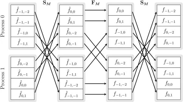
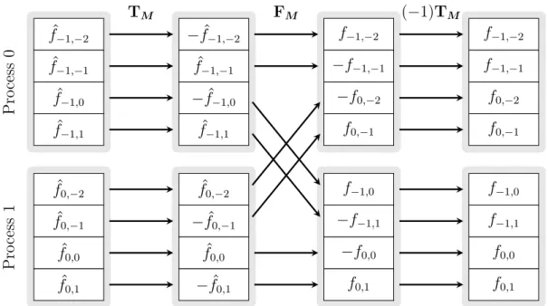
Finally, combination of (2.9) and (2.10) yields Algorithm 2.3 for the computation of the multidimensional pruned FFT with shifted index sets. The benefits of Algo-rithm 2.3 for parallel computations will become clear when we come to parallel data decomposition. A detailed discussion can be found in Sections 2.6 and 2.7.
Remark 2.4. A comparison of Algorithm 2.2 and Algorithm 2.3 reveals that a multidimensional pruned FFT can be easily extended to shifted index sets by the following three steps. First, we need to add a simple scaling of the FFT inputs and outputs given by the twiddle matrices Tmˆ and Tm in Algorithm 2.3. Second, we
replacePMt,mtˆ byPMt,e mtˆ , which means that the zero padding takes place at another
position in the input vectors. Last, the FFT outputs are truncated at a different po-sition due to the exchange ofPeT
Mt,mt forPTMt,mt. Therefore, we focus in the following
derivations on a parallel FFT framework based on the serial Algorithm 2.2. Once a parallel counterpart of Algorithm 2.2 is found, Algorithm 2.3 can be parallelized analogously by a simple exchange of PT
2.4 Basic modules for multidimensional array transformation 27
Algorithm 2.3 Multidimensional pruned FFT with shifted index sets
Input: ˆf ∈Cmˆ0···mdˆ −1,mˆ0, . . . ,mˆd−1 ∈2N . . . . 1: f ←Tmˆfˆ 2: for t =d−1, . . . ,0 do 3: f ←(Im0 ⊗ · · · ⊗Imt−1)⊗Pe T Mt,mtFMtPMt,e mtˆ ⊗(Imtˆ +1 ⊗ · · · ⊗Imˆd−1)f 4: end for 5: f ←Qdt=0−1(−1)(Mt+mt+ ˆmt)/2 ·Tmf . . . . Output: ˆf =PeTM,mSMFMSMPeM,mˆf ∈Cm0···md−1,mˆ0, . . . ,mˆd−1 ∈2N
Algorithm 2.4 Multidimensional pruned FFTH - Variant B
Input: f ∈Cm0···md−1 . . . . 1: fˆ←f 2: for t = 0, . . . , d−1 do 3: fˆ←(Im0 ⊗ · · · ⊗Imt−1)⊗PTMt,mtˆ FHMtPMt,mt ⊗(Imtˆ +1 ⊗ · · · ⊗Imˆd−1)fˆ 4: end for . . . . Output: ˆf =PTM,mˆFHMPM,mf ∈Cmˆ0···mˆd−1
Remark 2.5. So far we considered matrix factorizations and fast algorithms for computing DFTs. Note that the corresponding adjoint algorithms are immediately given by the adjoint matrix factorization of the DFT. For example, the adjoint factorization of (2.7) is given by
PT
M,mˆFHMPM,m =AHd−1· · ·AH0.
and yields Algorithm 2.4 for computing the multidimensional pruned FFTH; cf. the
non-adjoint Algorithm 2.2.
2.4 Basic modules for multidimensional array
transformation
Our parallel FFT framework will be a composition of several multidimensional array transformations. During these transformations the size of the data array may change and the dimensions of the array may be transposed. We will also see that all of these transformations can be realized in-place and out-of-place. In order to focus on the algorithmic workflow we introduce an appropriate shorthand notation that concen-trates on the absolutely essential details about the multidimensional transformations
and data layout. The starting point is that we abbreviate a fixed d-dimensional ar-ray g ∈CM0×···×Md−1 simply by its size M0 × · · · ×Md−1. Furthermore, we declare that arrays given in this notation are stored contiguously in memory following a linearized row-major order, i.e., the entry of g at position k= (kt)t=0d−1, 0 ≤kt< Mt
can be found in memory at position Pd−1
t=0 ktQdr=t+1−1 Mr. In the following, we will
see that this notation can be extended naturally to express the effects of several multidimensional array transformations.
2.4.1 The serial FFT module
Assume a three-dimensional input array ˆg∈Ch0×mˆ×h1. We introduce the notation
h0×mˆ ×h1 FFT→ h0×m×h1 (2.11)
to abbreviate an application of the matrixIh0⊗PTM,mFMPM,mˆ⊗Ih1, i.e., we compute
h0·h1 pruned one-dimensional FFTs along the second dimension ofgˆwith strideh1.
Note that we do not compute the one-dimensional FFTs along the first dimension h0. Later, we will useh0 to store the parallel distributed dimensions. The additional
dimension h1 at the end of the array allows us to compute a set of h1 serial FFTs
at once. We will see thath1 can be used in a higher-dimensional setting to store all
the dimensions where the FFT was already performed. Analogously, we define h0×m×h1 FFT→ h0×mˆ ×h1
as a set ofh0·h1 pruned one-dimensional adjoint FFTs along the second dimension
with stride h1. Note that the position of the hat distinguishes non-adjoint and
adjoint FFTs in our shorthand notation. This module can be implemented by one appropriately chosen FFTW plan. At this point it is important to recall that FFTW chooses the best suitable plan for a given problem and hardware out of a large collection of different FFT algorithms. Therefore, our serial FFT module inherits the automatic hardware adaptivity. Moreover, the application of FFTW introduces much flexibility to our serial FFT module. For example, this module can be executed in-place and applies fast O(MlogM) algorithms also for prime size FFTs.
Remark 2.6. For sake of simplicity, we restrict the serial FFT module to complex input data. However, the serial FFT transforms can be easily replaced by specialized FFT algorithms that take into account the additional symmetries of real input data as shown in [4]. In principle any one-dimensional transformation can be applied
instead of an FFT.
Remark 2.7. Note that the serial FFT module can be easily extended to support pruned FFT with shifted index sets. In this case it is sufficient to implement the matrix operation given by Ih0 ⊗PeTM,mFMPM,e mˆ ⊗Ih1, see also Remark 2.4.
2.4 Basic modules for multidimensional array transformation 29
2.4.2 The local transposition module
The following shorthand notation describes a transposition of a three-dimensional array gˆ∈Ch0×mˆ×h1 along its first two dimensions
ˆ m×h0×h1 → TI h0×mˆ ×h1 (2.12) and h0×mˆ ×h1 → TOmˆ ×h0×h1. (2.13)
Thereby, we can choose whether the input (TI) or the output (TO) array should be transposed, respectively.
This module can be realized by a single appropriately chosen FFTW plan. Al-though array transposition is a standard task in matrix computations, its efficient implementation is indeed a nontrivial task. Especially, one has to think of many details about the memory hierarchy of current computer architectures. At this point, we benefit of the cache oblivious array transpositions [59] that are imple-mented within FFTW. This means that the asymptotic number of cache misses is minimized independently of the cache size.
2.4.3 Combination of serial FFT and local transposition
A combination of the serial FFT module (2.11) and local transpositions (2.12), (2.13) results in the following two three-dimensional array transformations
ˆ
m×h0×h1 FFT→
TI h0×m×h1, h0×mˆ ×h1 FFT→
TO m×h0×h1. (2.14)
Both realize a set of pruned one-dimensional FFTs. However, the first one starts with an input array that is transposed in the first two dimensions, while the second one ends up in a transposed output array. Note that we do not specify the order of execution between the transposition and the FFTs a priori. For example, we can implement the first transform with only one appropriate chosen FFTW plan. But we are also free to use two successive plans to perform the serial FFT first and the transpose in the second step as
ˆ
m×h0 ×h1 FFT→ m×h0×h1 →TI h0 ×m×h1
or the other way around as follows ˆ
m×h0×h1 →
TI h0×mˆ ×h1 FFT
→ h0×m×h1.
We leave it to a planner to find the fastest of these three algorithms at runtime. The serial FFT with transposed output is handled analogously.
0 1 2 3 4 5 6 7 Process 0 [M/P]3 0 Process 1 [M/P]3 1 Process 2 [M/P]3 2 Process 3 [M/P]3 3
Figure 2.3: An array of sizeM = 8 gets block decomposed onP = 4 processes with block size B = 3. The picture shows the resulting local blocks [M/P]B j
for all processes j ∈ {0,1,2,3}.
2.4.4 Parallel block decomposition
In the following, we introduce the data decomposition that is used for our parallel FFT algorithms. We start with the definition of a one-dimensional block decomposi-tion. Afterward, we discuss the straightforward generalization to higher-dimensional settings.
Assume a one-dimensional array ˆg= (ˆgk)Mk=0−1 of complex numbers that should be
distributed on P ∈ N processes. We use the notation [M/P]Bj to symbolize that all
data elements ˆgk with jB ≤ k < (j + 1)B belong to process j ∈ {0, . . . , P −1}.
Hereby, the block size B ∈ N must be chosen B ≥ M/P such that no data remains
undistributed. We see that the first dM/Be processes get contiguous data blocks
of block length B. Thereby, we used the notation dxe := min{z ∈ Z : x ≤ z} for rounding x ∈ R up. For the sake of convenience, we skip the index j in the aforementioned block notations whenever a statement is valid for all processes j = 0, . . . , P −1. This means [M/P]B can be read as [M/P]B
j for all j = 0, . . . , P −1.
Analogously, we skip the block sizeB whenever a statement is valid for any integer block size B ≥ M/P. Figure 2.3 shows an example of a one-dimensional block
decomposition.
Of course, we are interested in block sizes that imply an almost equal data dis-tribution on all processes. One way to choose the block size automatically is to set the default value B =dM/Pe in correspondence to the definition of the parallel
FFTW interface. If M is divisible by P, the default block size is simply B = M/P
and results in P equal pieces each consisting of M/P contiguous data elements of gˆ
as illustrated in Figure 2.4.
Multidimensional block decompositions are defined straightforward by the blocks that result from one-dimensional block decomposition along each dimension. In combination with the shorthand array notation that was introduced at the beginning of Section 2.4 we are now able to express multidimensional arrays that are block distributed along several dimensions. For example, assume a three-dimensional array (ˆgk0,k1,k2)
M0−1,M1−1,M2−1
k0,k1,k2=0 of sizeM0×M1×M2 that is block distributed on a Cartesian
process mesh of sizeP0×P1along the first two dimensions. Then, we write [M0/P0]B0
i ×
[M1/P1]B1
2.4 Basic modules for multidimensional array transformation 31 0 1 2 3 4 5 6 7 Process 0 [M/P]2 0 Process 1 [M/P]2 1 Process 2 [M/P]2 2 Process 3 [M/P]2 3
Figure 2.4: An array of sizeM = 8 gets block decomposed on P = 4 processes with default block size B = 2. The picture shows the resulting local blocks [M/P]B
j for all processes j ∈ {0,1,2,3}. Since M is divisible by P, the
default block size decomposition yields perfect load balancing.
0 1 2 3 4 5 6 7 8 9 10 11 12 13 14 15 16 17 18 19 20 21 22 23 j = 0 j = 1 j = 2 i= 0 i= 1
Process mesh columns
Pro cess me sh ro ws
Figure 2.5: A two-dimensional array of sizeM0×M1 = 3×8 gets block decomposed
on a two-dimensional process mesh of sizeP0×P1 = 2×3 with default
block sizes B0 = 2 and B1 = 3. The picture shows the mapping of the
local array blocks [M0/P0]B0
i ×[M1/P1]Bj1 to each process (i, j). Hereby, i
and j are running indexes along the process mesh rows and columns, respectively.
all data ˆgk0,k1,k2 withiB0 ≤k0 <(i+ 1)B0,jB1 ≤k1 <(j+ 1)B1, and 0≤k2 < M2.
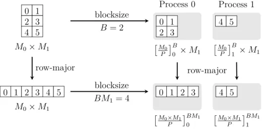
Thereby, we declare all data blocks to be stored in row-major order. In Figure 2.5 we present an illustration of a two-dimensional block decomposition with unequal block sizes. Furthermore, we define the notation [(M0×M1)/P]B
j by a one-dimensional
block decomposition that results from the following two steps. First, linearize the two-dimensional array M0×M1 in row-major order and, second, block decompose
this linearized array on P processes with block size B. In this case, block size B ≥M0M1/P must be fulfilled in order to distribute all data.
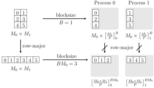
2.4.5 Folding multidimensional arrays in row-major order
An important observation is that an one-dimensional block decomposition of a two-dimensional array can be interpreted as a block decomposed one-two-dimensional array with suitably chosen block size. More precisely, let a size M0×M1 array be block