Riemannian Optimization for Convex and Non-Convex Signal Processing and Machine Learning Applications

(1)

Signal Processing and Machine Learning Applications

Thesis by

Ahmed Douik

In Partial Fulfillment of the Requirements for the Degree of

Doctor of Philosophy

CALIFORNIA INSTITUTE OF TECHNOLOGY Pasadena, California

2020

(2)

(3)

ACKNOWLEDGEMENTS

Firstly, I would like to express my sincere gratitude to my advisor Prof. Babak Hassibi for the continuous support of my Ph.D research, for his motivation, and immense knowledge.

Besides my advisor, I would like to thank the rest of my thesis committee, Prof. P. P. Vaidyanathan, Prof. V. Kostina, Prof. J. Tropp and, Prof. V. Chandrasekaran, for their insightful and valuable comments and encouragement.

Finally, I would like to also thank my fellow labmates and friends from Caltech for the stimulating discussions and for all the fun we have had in the last five years.

(4)

ABSTRACT

The performance of most algorithms for signal processing and machine learning applications highly depends on the underlying optimization algorithms. Multiple techniques have been proposed for solving convex and non-convex problems such as interior-point methods and semidefinite programming. However, it is well known that these algorithms are not ideally suited for large-scale optimization with a high number of variables and/or constraints. This thesis exploits a novel optimization method, known as Riemannian optimization, for efficiently solving convex and non-convex problems with signal processing and machine learning applications. Unlike most optimization techniques whose complexities increase with the number of constraints, Riemannian methods smartly exploit the structure of the search space, a.k.a., the set of feasible solutions, to reduce the embedded dimension and efficiently solve optimization problems in a reasonable time. However, such efficiency comes at the expense of universality as the geometry of each manifold needs to be investigated individually. This thesis explains the steps of designing first and second-order Riemannian optimization methods for smooth matrix manifolds through the study and design of optimization algorithms for various applications. In particular, the paper is interested in contemporary applications in signal processing and machine learning, such as community detection, graph-based clustering, phase retrieval, and indoor and outdoor location determination. Simulation results are provided to attest to the efficiency of the proposed methods against popular generic and specialized solvers for each of the above applications.

(5)

PUBLISHED CONTENT AND CONTRIBUTIONS

[1] A. Douik et al. “Precise 3-D GNSS Attitude Determination Based on Rie-mannian Manifold Optimization Algorithms”. In: IEEE Transactions on Signal Processing 68.1 (Dec. 2020), pp. 284–299. doi: 10 . 1109 / TSP . 2019.2959226.

Ahmed Douik participated in the conception of the project, designed and im-plemented the optimization algorithm, helped with simulations, and wrote parts of the manuscript.

[2] A. Douik and B. Hassibi. “Manifold Optimization Over the Set of Doubly Stochastic Matrices: A Second-Order Geometry”. In:IEEE Transactions on Signal Processing67.22 (Nov. 2019), pp. 5761–5774. doi:10.1109/TSP. 2019.2946024.

Ahmed Douik participated in the conception of the project, solved the problem, designed the algorithm, prepared the simulations, and wrote the manuscript.

[3] A. Douik and B. Hassibi. “Non-Negative Matrix Factorization via Low-Rank Stochastic Manifold Optimization”. In:Proc. of the IEEE International Sym-posium on Information Theory (ISIT’ 2019), Paris, France. Vol. 1. 1. June 2019, pp. 497–501. doi:10.1109/ISIT.2019.8849441.

[4] A. Douik, F. Salehi, and B. Hassibi. “A Novel Riemannian Optimization Approach and Algorithm for Solving the Phase Retrieval Problem”. In: Proc. of the 53rd Asilomar Conference on Signals, Systems, and Computers (Asilomar’ 2019), Asilomar, CA, USA. Vol. 1. 1. Nov. 2019, pp. 1962–1966. doi:10.1109/IEEECONF44664.2019.9049040.

Ahmed Douik participated in the conception of the project, studied the prob-lem, designed and implemented the algorithm, helped with the simulations, and wrote parts of the manuscript.

[5] A. Douik and B. Hassibi. “A Riemannian Approach for Graph-Based Clus-tering by Doubly Stochastic Matrices”. In: Proc. of the IEEE Statistical Signal Processing Workshop (SSP’ 2018), Freiburg, Germany. Vol. 1. 1. June 2018, pp. 806–810. doi:10.1109/SSP.2018.8450685.

[6] A. Douik and B. Hassibi. “An Improved Initialization for Low-Rank Matrix Completion Based on Rank-1 Updates”. In:Proc. of the IEEE International Conf. on Acoustics Speech and Signal Processing (ICASSP’ 2018), Calgary,

(6)

AL, Canada. June 2018, pp. 1–5. doi:10.1109/ICASSP.2018.8461826. Ahmed Douik participated in the conception of the project, designed and implemented the initialization, prepared the simulations, and wrote the manuscript.

[7] A. Douik and B. Hassibi. “Low-Rank Riemannian Optimization on Pos-itive Semidefinite Stochastic Matrices with Applications to Graph Clus-tering”. In: Proc. of the International Conference on Machine Learning (ICML’ 2018), Stockholm, Sweden. Vol. 80. July 2018, pp. 1299–1308. url: proceedings.mlr.press/v80/douik18a.html.

(7)

LIST OF ILLUSTRATIONS

Number Page

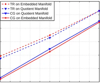
2.1 The update step for the two-dimensional sphere embedded in_R3. . . . 14 2.2 Tangent space of a 2-dimensional manifold embedded in_R3. . . 15 3.1 Running time of the different non-convex clustering algorithms. . . . 49 4.1 Accuracy of Riemannian methods for clustering a large system. . . . 75 4.2 Running time of Riemannian methods for clustering a large system. . 75 4.3 Accuracy of Riemannian methods against the number of clusters. . . 76 4.4 Convergence rate of the conjugate gradient algorithm onM𝑛

𝑝andM 𝑛 𝑝. 77

4.5 Convergence rate of the trust-region algorithm onM𝑛

𝑝andM 𝑛

𝑝. . . . 78

4.6 Performance of Algorithm 4.1 and Algorithm 4.2. . . 78 4.7 Performance of the different NMF algorithms. . . 88 4.8 Running time to decompose the ORL and the CBCL face databases. . 88 5.1 Running time to solve the Fourier phase retrieval problem. . . 107 5.2 Accuracy in the reconstruction of the Fourier phase retrieval problem. 108 6.1 A localization system consisting of 3 transmitters and 4 receivers. . . 112 6.2 Mean square error of the location estimate. . . 125 6.3 Value of the cost function at the reached solution. . . 125 6.4 CDF of the location error under maximum ranging error of 35 mm. . 126 6.5 Running time to estimate the location of the target. . . 126 6.6 Receiver antenna configuration for ambiguity resolution. . . 131 6.7 Receiver antenna configuration for 3-D attitude determination. . . 133 6.8 Fraction of estimates with error less than𝜖 over different GPS weeks. 149 6.9 Root mean square error versus noise levels (29/4/2018). . . 149 6.10 Root mean square error versus the number of satellites (29/4/2018). . 149 6.11 Root mean square error versus the angle (29/4/2018). . . 150

(9)

LIST OF TABLES

Number Page

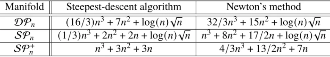
2.1 Riemannian embedded and quotient manifolds notations. . . 13 3.1 Complexity of the steepest-descent algorithm and Newton’s method. . 42 3.2 Execution time of the doubly stochastic multinomial manifold. . . 45 3.3 Execution time of the symmetric multinomial manifold. . . 45 3.4 Execution time of the definite multinomial manifold. . . 46 3.5 Performance of the Riemannian methods for convex clustering. . . . 47 4.1 Performance of the Riemannian methods for non-convex clustering. . 74 6.1 Success rates over many GPS weeks. . . 147 6.2 Root mean square error over different GPS weeks. . . 147 6.3 Performance of different GNSS attitude determination algorithms. . . 151

(10)

LIST OF ALGORITHMS

Number Page

2.1 Template of optimization algorithms on Riemannian manifolds. . . . 14 2.2 Template of the gradient descent procedure on Riemannian manifolds. 21 2.3 Template of Newton’s method on Riemannian manifolds. . . 21 2.4 Template of the conjugate gradient method on Riemannian manifolds. 22 4.1 Steepest-descent algorithm on the manifoldM𝑛

𝑝. . . 72

4.2 Newton’s method on the manifoldM𝑛𝑝. . . 73

5.1 Gradient descent on the fixed norms manifold. . . 107 6.1 Riemannian steepest-descent on the equilateral triangle manifold. . . 123 6.2 Algorithm for 3-D GNSS attitude determination. . . 145

(11)

LIST OF ACRONYMS

A-HALS Accelerated Hierarchical Alternating Least Squares. 87–89 A-MU Accelerated Multiplicative Updates. 87–89

A-PGM Accelerated Projected Gradient Method. 87 ALM Augmented Lagrange Multipliers. 74

ALS Alternating Least Squares. 87–89

ANLS Alternating Nonnegative Least Squares. 87–89 AoA Angle of Arrival. 110, 111, 131

ARC Adaptive Regularization with Cubics. 124 BFGS Broyden–Fletcher–Goldfarb–Shanno. 46 BHHH Berndt-Hall-Hall-Hausman. 46

CG Conjugate Gradient. 4, 74, 87 DFT Discrete Fourier Transform. 91 DoP Dilution of Precision. 148 END East-North-Down. 6 ENU East-North-Up. 6 GN Gauss-Newton. 124, 125

GNSS Global Navigation Satellite Systems. 5–8, 127–132, 134, 144, 147 GPS Global Positioning System. 147–150

GSO Gram-Schmidt Orthonormalization. 128

HALS Hierarchical Alternating Least Squares. 87–89 IoT Internet of Things. 6

(12)

IPM Interior-Point Method. 44–46, 122, 126 KKT Karush-Kuhn-Tucker. 54, 57 LRM Low-Rank Multinomial. 87–89 LS Least Squares. 132, 145–147, 149–151 LU Lower–Upper. 43 MM Majorize Minimization. 49 MSE Mean Square Error. 124–126 MU Multiplicative Updates. 87, 89

NMF Non-negative Matrix Factorization. 80, 87, 89 PGM Projected Gradient Methods. 87

PSD Positive Semidefinite. 53, 54

RAM Random Access Memory. 44, 74, 124 RMSE Root Mean Square Error. 148, 150, 151 RSS Received Signal Strength. 110

SNR Signal-to-Noise Ratio. 88, 124

SQP Sequential Quadratic Programming. 44–47, 122, 126 SVD Singular Value Decomposition. 80

TDoA Time Difference of Arrival. 112 ToA Time of Arrival. 111

ToF Time of Flight. 109–111

(13)

C h a p t e r 1

INTRODUCTION

Optimization is a fundamental and crucial tool for most signal processing and ma-chine learning applications. Several classes of optimization have been identified in the literature, e.g., discrete [1], non-smooth [2], and derivative-free [3] optimiza-tion. For its numerous applications, this thesis only focuses onsmooth continuous optimization, denoted simply by the generic term “optimization" in the rest of the thesis. Historically initiated with the study of least-squares and linear programming problems [4], convex optimization is an essential subclass of optimization problems in which both the objective function and the search set, i.e., constraints, are convex. As the successor and the generalization of linear programs, convex optimization received significant attention from the research community thanks to the desirable convergence property it exhibits. As a matter of fact, under mild conditions, well-defined and explicit convex problems can be solved numerically efficiently [5]. As such, it has been successfully and extensively used in numerous applications, re-gardless of their convexity [6]. Indeed, while the actual applications may not be convex, reformulating or approximating the problem by a convex program has been a successful approach to obtaining “good-enough" solutions. Such a strategy is known in the scientific literature as aconvex relaxationof the problem [7].

Despite their relative success, relying on relaxations and convex solvers might lead to poor performance in some instances. Indeed, while convex relaxations can induce an unwanted degradation in the quality of the solution, it has been established that convex methods are excessively slow for high dimensions. In other words, they suffer from the curse of dimensionality. As such, it has been observed that for some contemporary signal processing and machine learning applications, non-convex solvers are significantly more efficient than their convex counterparts both in terms of quality of the solution and convergence time [8]. Such behavior is primarily due to the fact that non-convex methods successfully exploit the structure of the problem, which is destroyed in the convex reformulation/approximation. Therefore, proposing non-convex solvers has been an emerging and captivating research topic of late, e.g., see [9, 10] and references therein.

(14)

non-convex constrained optimization problems. These algorithms include the cel-ebrated interior-point methods [11], semi-definite programming [5], Lagrangian multiplier methods [12], and simpler approaches such as alternating minimization algorithms [13, 14], including alternating orthogonal projection [15]. While these algorithms have the merit of being both generic and easily implementable, their convergence might be excessively time-consuming for high-dimensional convex problems. Furthermore, the performance of these algorithms is largely unknown for non-convex programs.

This thesis presents an alternative optimization method that circumvents both above-identified limitations, i.e., poor solution’s quality and high complexity, resulting in highly efficient convex and non-convex optimization algorithms. The optimization method, known as Riemannian optimization, solves the constrained optimization problem as an unconstrained one over a restricted search space. This restriction of the search space allows the solution to be feasible while reducing the dimension of the problem, thus providing Riemannian optimization with exceptional abilities in finding efficient solutions in a reasonable time. However, the same mechanism introduces curvature as the search space is no longer Euclidean, which hinders the universality of the method for the geometry of each manifold needs to be investigated individually. To that end, this paper explains the steps of designing first and second-order Riemannian optimization methods for smooth matrix manifolds through the study and design of optimization algorithms for various contemporary applications in signal processing and machine learning.

1.1 Introduction to Riemannian Optimization Methods Unconstrained and Riemannian Optimization Methods

As stated earlier, numerical optimization is the foundation of various engineering and computational sciences. Consider a smooth map f from a subset D of _R𝑛

to

R. The goal of optimization algorithms is to discover an extreme point x∗ ∈ D

such that f(x∗) ≤ f(y) for all feasible points y ∈ Nx∗ in the neighborhood of x∗.

These traditional optimization schemes in which the embedding space is linear, such as the space of real vectors R𝑛 and matrices R𝑛×𝑚, are identified with the

term Euclidean in contrast with the Riemannian algorithms in the rest of the paper. While unconstrained Euclidean optimization refers to the setup in which the domain of the objective function is the whole space, i.e., D = _R𝑛

, constrained Euclidean optimization denotes problems in which the search set is restricted, i.e.,D ₍_R𝑛

(15)

This manuscript is interested in the generic class of optimization problems in which the interior of the search space can be identified with a manifold that is embedded in a higher-dimensional Euclidean space, e.g., low-rank matrices embedded in the Euclidean space of matrices _R𝑛×𝑚

. While such problems can be solved using constrained optimization methods [11], these algorithms can be excessively slow as they require solving on the high-dimensional Euclidean space. Riemannian optimization takes advantage of the fact that the manifold is of lower dimension and exploits its underlying geometric structure to reduce the computation complexity significantly.

The above property is achieved by extending unconstrained optimization schemes from Euclidean spaces to Riemannian manifolds. As such, Riemannian optimiza-tion methods fall within the scope of iterative optimizaoptimiza-tion algorithms. In other words, starting from an initial position, the algorithm sequentially finds a series of neighboring points that converge to a critical point of the optimization objective function. However, unlike the interior-point method and similar algorithms that modify the objective function by including a barrier or additional (dual) variables, the philosophy of Riemannian optimization is to solve the constrained optimization problem as an unconstrained one over a restricted search space. Indeed, by reformu-lating the problem as a minimization over the set defined by the constraints, called thesearchor thefeasible space, the problem can be thought of as an unconstrained optimization over a constrained set, known as the manifold.

Thanks to the aforementioned low-dimension feature, optimization over Riemannian manifolds is expected to perform more efficiently [16] than traditional optimization approaches. Therefore, a large body of literature has been dedicated to adapting traditional Euclidean optimization methods and their convergence properties to Riemannian manifolds. The rest of this section provides an overview of such rich Riemannian optimization literature along with the achieved milestones.

History, Merits, and Limitations of Riemannian Optimization

Riemannian optimization algorithms appeared in the literature for the first time in the 1970s work of Luenberger [17] by the adaptation of the standard Newton’s method to Riemannian manifolds. The author demonstrated that the Riemannian version of Newton’s method exhibits quadratic convergence. However, such guarantees come at a high complexity price per iteration. Indeed, finding the search direction requires computing the exact Hessian using parallel vector transport, and the step

(16)

size is optimized by searching along the geodesic, i.e., straight line on a Riemannian manifold. The complexity is partially reduced for embedded submanifolds ofR𝑛

with the work of Gabay [18] which introduces the steepest-descent and the quasi-Newton algorithms and demonstrate their convergence for embedded submanifolds of_R𝑛

.

The convergence results of the steepest-descent and the quasi-Newton in [18] are extended from embedded submanifolds of R𝑛 to abstract Riemannian manifolds

[19, 20]. Although these approaches are notably faster than the standard Newton’s method, they are far from competing with established constrained optimization algorithms. The first breakthrough in the field happens with the substitution of the complex exact line-search by the effective Armijo step-size control while preserving the convergence rate. Such improvement allows the design of a unified framework for constrained and unconstrained optimization [21]. Another notable improvement for the quasi-Newton algorithms is the use of a general connection as an alternative to the canonical parallel vector transport for computing the approximate Hessian. However, while the modified algorithm conserves its global convergence property, it no longer ensures a superlinear convergence rate [22].

All above-mentioned Riemannian optimization works extend the unconstrained schemes to Riemannian manifolds by, inter alias, replacing the line-search part with the natural and intuitive search along the straight lines of the manifolds, viz., geodesics. The expression of these geodesics is acquired from the exponential map, which may be more challenging to derive than solving the original optimization problem [23]. The authors in [24] achieved the second breakthrough in Riemannian optimization by showing that Newton’s method conserves its quadratic convergence rate when using a second-order approximation of the exponential map, known as a retraction.

With multiple efforts from the Riemannian optimization community, e.g., [25, 26, 27, 28], the result of [24] has been extended to first-order retractions and more-sophisticated optimization algorithms such as the CG and TR methods. These algorithms have been successfully implemented to efficiently solve various problems in communication and signal processing such as clustering or community detection [29, 30, 31, 32] and low-rank matrix completion [33, 34, 35, 36].

Thanks to its high efficiency in solving sizeable convex and non-convex programs, Riemannian optimization is slowly but surely gaining momentum in the optimiza-tion literature [16]. However, its use by the scientific community at large remains

(17)

relatively limited mainly due to the non-universality of the method and the required pre-requisite knowledge of differential geometry and Riemannian manifolds. In-deed, as the technique relies on the structure of the problem and due to the lack of a systematic mechanism to design optimization algorithm over manifolds, its use might be prohibitively complicated for non-experts in the field. Nonetheless, thanks to the implementation of multiple optimization algorithms over a broad set of manifolds, e.g., the MATLAB optimization framework ManOpt [37], Riemannian optimization is becoming more and more user-friendly.

1.2 Signal Processing and Machine Learning Problems of Interest

This manuscript exploits Riemannian optimization techniques to solve multiple problems in signal processing and machine learning. These applications include convex and non-convex graph-based clustering [38], also known as the similarity clustering [39, 40, 41] by doubly stochastic matrices, Fourier phase retrieval [42, 43, 44], indoor high-accuracy spatial location and orientation estimation using ultrasound waves [45, 46, 47], and outdoor precise attitude determination in the Global Navigation Satellite Systems (GNSS) [48, 49, 50, 51, 52].

Clustering by Doubly Stochastic Matrices

Convex and non-convex optimization over the set of doubly stochastic matrices has numerous applications in signal processing and machine learning applications for its close relationship with graph theory and Markov chains. One of the most popular application of doubly stochastic matrices in machine learning is graph-based clustering [39, 53, 54, 55] wherein one wishes to separate data points into different groups, known as clusters. Similarity clustering is a subset of clustering applications in which one is given an entry-wise non-negative similarity matrixAbetween𝑛data points with the goal of clustering these data points into𝑟 clusters. Multiple convex, e.g., [39], and non-convex, e.g., [53], approaches have been proposed to solve the similarity clustering problem. This thesis provides a unified framework to carry such optimization.

Fourier Phase Retrieval

Phase retrieval is a classical problem in signal processing [42] in which one wishes to recover a complex signal from observations of the amplitude of linear combinations of the signal. The problem is crucial in multiple imaging applications wherein the phase of the signal cannot be measured for technical or economic reasons.

(18)

Indeed, due to the inability of physical measurement devices to detect phases, e.g., a photosensitive film that measures the light intensity, only the magnitude of the signal is available. These applications include optics, crystallography, astronomical imaging, speech processing, computational biology, and blind deconvolution. Phase retrieval engaged several researchers over the years with numerous theoretical results [43, 56] and practical algorithms [57]. This manuscript focuses on the popular case of Fourier phase retrieval [58, 59] in which a subset of the available observations are obtained through the Fourier transform of the signal. This particular structure of the phase retrieval problem allows its reformulation as a constrained optimization problem wherein the constraint set is represented by an orthonormal basis. This paper demonstrates how to effectively exploit the structure of the problem to speed up its solution.

Spatial Location Estimation Using Ultrasound Waves

With the rapidly increasing number of smartphones and the proliferation of the Internet of Things (IoT), location-based services gained an increased interest in the last decade [60]. These services range from outdoor localization, e.g., for naviga-tion purposes, to accurate indoor pinpointing for applicanaviga-tions such as robot steering, surveillance, video gaming, and virtual reality [61]. While outdoor localization is universally solved by the GNSS, such a system is not feasible indoors. As such, indoor localization systems have been implemented using various competing tech-nologies, including ultrasound waves [62], radio-frequency [63], infrared radiation [64], and laser signals [65].

For most localization systems, a small perturbation in the measurement can result in a significant deviation in the expected location, especially under a bad geometry [66]. To circumvent the aforementioned limitation, this manuscript aims to design a novel and highly accurate spatial location estimation method that uses multiple transmitters and considers exploiting their geometry in the estimation process. The resulting transmitter diversity not only significantly improves the accuracy of the estimated location but also provides the 3D orientation of the device.

Attitude Determination in Global Navigation Satellite Systems

The goal of attitude determination is to estimate the orientation of a vehicle relative to the selected coordinate system, such as the East-North-Up (ENU) frame or the East-North-Down (END) frame. The 3-D attitude information can be represented using Euler angles (yaw, pitch, and roll), which can be uniquely determined by

(19)

three or more non-collinear GNSS receivers. These receivers collect two types of measurements, pseudo-range and carrier phase. Carrier phase measurements are several orders of magnitude more accurate than pseudo-ranges, but are subject to ambiguities due to unknown (integer) number of unobserved wavelength cycles [67]. Therefore, phase ambiguity resolution is a critical process for high-accuracy attitude determination. After successfully resolving the ambiguity, the carrier phase can be utilized to precisely estimate direction vectors of the receiver baselines [68]. The estimation can be enhanced by leveraging geometrical information of the receiver configuration, as well as the unitary nature of the direction vectors of interest. This manuscript uses Riemannian optimization techniques to obtain the baseline’s direction vectors, which can be directly converted into Euler angles to fully characterize the attitude of the platform.

1.3 Contributions, Notations, and Organization Scope and Contributions

The main contribution of this paper is to exploit Riemannian optimization methods to design efficient optimization algorithms to solve the aforementioned convex and non-convex problems in signal processing and machine learning. However, such en-deavor requires some level of knowledge of differential and Riemannian geometries. To that end, the manuscript provides an introduction on designing efficient first and second-order Riemannian optimization methods for smooth matrix manifolds. As only smooth embedded and quotient matrix manifolds are considered, the definitions and theorems herein may not apply to abstract manifolds. In addition, the author opted for a coordinate-free analysis omitting charts and differentiable structures of manifolds. For an introduction to differential geometry, abstract manifolds, and Riemannian manifolds, we refer the readers to the following references [69, 70, 71], respectively.

After introducing the necessary machinery to design Riemannian optimization algo-rithm, this thesis investigates the aforementioned convex and non-convex clustering, phase retrieval, and localization applications. In particular, the doubly stochastic and symmetric stochastic multinomial manifolds are introduced and their geome-tries investigated so as to design efficient convex clustering algorithms. Afterwards, the low-rank property of the solution to the clustering problem is exploited to re-formulate the community detection task as a non-convex program. The non-convex reformulation is solved by providing theoretical guarantees on the quality of the solution and investigating the geometry of the low-rank symmetric stochastic

(20)

multi-nomial.

For the phase retrieval problem, the feasible set is represented by generic quadratic equations. While there is no guarantees that such set admits a manifold structure in general, the manuscript shows that the set of feasible solutions represents a Rieman-nian manifold under Fourier observations. The first and second-order geometries of the newly introduced manifold, known as the fixed norms manifold, are investigated and efficient phase retrieval algorithms are designed. Furthermore, by exploiting the fact that the optimization problem for phase retrieval presents non-isolated solutions, the manifold is demonstrated to admit a quotient structure, allowing the design of even faster algorithms.

Afterwards, the thesis investigates and designs indoor and outdoor precise localiza-tion systems. For instance, the problem of accurate indoor spatial localocaliza-tion and ori-entation estimation using ultrasound waves is considered. To improve the accuracy of the localization system, the transmitters’ geometry is integrated into the loca-tion estimaloca-tion process by formulating the problem as a non-convex optimizaloca-tion. Afterward, the set of feasible solutions is shown to admit a Riemannian manifold structure, which allows solving the underlying optimization problem rigorously. Finally, outdoor localization is examined through the problem of altitude determina-tion in GNSS. The antenna geometry and baseline lengths are exploited to formulate the 3-D GNSS attitude determination problem as an optimization over a non-convex set, shown to be a manifold. The study of the geometry of the manifold allows the design of efficient first and second-order Riemannian algorithms to solve the 3-D GNSS attitude determination problem.

Organization

The rest of this manuscript is organized as follows. Chap. 2 introduces Riemannian manifolds and optimization techniques. These techniques are utilized in Chap. 3 to design efficient optimization algorithms for convex graph-based clustering. The results are extended to low-rank matrices in Chap. 4 so as to tackle non-convex community detection. The Fourier phase retrieval problem is investigated in Chap. 5. Finally, before concluding in Chap. 7, accurate indoor and outdoor localization algorithms are designed in Chap. 6.

(21)

Notations

Throughout the paper, lower-case letters 𝑥 denotes scalar variables, while bold-face lower-case letters x and boldface upper-case X denote vectors and matrices, respectively. Tangent vectors and matrices are an exception to the previous rule and are denoted by Greek letters with an index representing the foot of the tangent space, e.g.,𝜉_xrepresents a tangent vector atx. These Riemannian geometry related notations would become more apparent in Chap. 2.

The𝑖-th entry of vectorxis denoted byx𝑖 and the element in the𝑖-th row and 𝑗-th

column of matrix Xis denoted by X𝑖 𝑗. The notations 0, 1, and I denote the null

vector, the all ones vector, and the identity matrix, respectively. If the dimension of the vector is not clear from the context, it is added as a subscript. For example,I𝑛

denote the identity matrix of size𝑛×𝑛. Given a vectorx, the symbols|x|,xT, andx★

denote the absolute value, the transpose and the conjugate transpose operators of vectorx, respectively. The absolute value of a vector is defined as the absolute value of each of its entries. For a matrix X, the notations kXk, XT, andXH denotes the Frobenius norm, the transpose and the Hermitian operators of matrixX, respectively.

While sets are denoted by a calligraphic font, e.g.,X, the sets of real and complex numbers are denoted byRandC, respectively. The set of real and complex vectors

and matrices follow the usual notation of placing the dimension as exponents. For instance,_R𝑛×𝑚

refers to the set of real matrices of size𝑛×𝑚. Given a symmetric (or Hermitian) matrixX=XT(orX=XH), the notationX 0means that matrix is positive-definite, i.e., all its eigenvalues are strictly positive. Likewise, the symbol X > 0 refers to a real matrixX ∈ _R𝑛×𝑚 with strictly positive entries, i.e., X𝑖 𝑗 > 0

for all 1 ≤𝑖 ≤ 𝑛and 1 ≤ 𝑗 ≤ 𝑚.

Let the notation Tr(.) refer to the trace operator and hX,Yi = Tr(YTX) to the Frobenius inner product of matricesXandYon the spaceR𝑛×𝑛. Given two matrices,

the element-wise product, a.k.a., the Hadamard product, is denoted by the symbol , i.e., (XY)𝑖 𝑗 = X𝑖 𝑗Y𝑖 𝑗. Similarly, the Hadamard division is denoted by the

symbol. LetS𝑛

andS𝑛

skew be the set of symmetric and skew-symmetric matrices,

respectively. A full-rank 𝑛× 𝑝 matrix Y is an element of the set_R𝑛×𝑚

★ . The set

O𝑝

={O∈_R𝑝×𝑝 ★ |OO

T ₌_I_}_{represents orthogonal matrices.}

Functions are denoted by lower- and upper-case letters with sans serif font. Addi-tionally, Greek letters are used to denote functions representing curves on manifolds.

(22)

To explicitly mention the pre-image and image sets by a function F, the standard notationF:X → Yis used. For a single variable function, e.g.,𝛾(𝑡), the shorthand notation𝛾¤(𝑡) is used to denote the first-order derivative𝛾¤(𝑡) = d

𝛾 d𝑡.

The set of continuously differentiable is denoted byC1. Similarly, the symbolC2is used to refer to the class of all first and second continuously differentiable functions. In the rest of the manuscript, a smooth function refers to a function of class at least C1_{for first-order algorithms and at least}_C2_{for second-order methods.}

(23)

C h a p t e r 2

OPTIMIZATION ON RIEMANNIAN MANIFOLDS

This chapter introduces Riemannian optimization methods on embedded and quo-tient Riemannian matrix manifolds. In particular, Section 2.1 presents the manifold definitions and notations used throughout the thesis. Afterward, the geometries of embedded and quotient matrix submanifolds are investigates in Sections 2.2 and 2.3, respectively. Finally, Section 2.4 exploits such geometries to design various first and second-order Riemannian optimization algorithms.

2.1 Manifold Definitions and Notation

The philosophy of Riemannian optimization techniques is to extend unconstrained optimization methods from Euclidean spaces to manifolds. As such, this part first recalls the principals of Euclidean optimization. Afterward, Riemannian matrix manifolds and submanifolds are introduced. Finally, an overview of Riemannian optimization methods is presented. For clarity purposes, the optimization over linear spaces, i.e., Euclidean spaces, is refereed as Euclidean optimization with contrast with Riemannian optimization.

Euclidean Spaces and Optimization

The general idea behind unconstrained Euclidean numerical optimization methods is to start with an initial point X0 and to iteratively update it according to certain predefined rules in order to obtain a sequence {X𝑡

}∞

𝑡=0 which converges to a local

minimum of the objective function. A typical update strategy isX𝑡+1 = X𝑡

+𝛼𝑡𝑝𝑡 where𝛼𝑡is the step size and𝑝𝑡the search direction. LetGrad f(X)be the Euclidean gradient of the objective function defined as the unique vector satisfying:

hGrad f(X), 𝜉i=D f(X) [𝜉], ∀𝜉 ∈ E,

whereh., .iis the inner product on the vector spaceEandD f(X) [𝜉]is the directional derivative of 𝑓 given by:

D f(X) [𝜉] =lim

𝑡→0

f(X+𝑡 𝜉) −f(X)

𝑡

.

In order to obtain a descent direction, i.e.,f(X𝑡+1₎

< f(X𝑡) for a small-enough step size𝛼𝑡, the search direction 𝑝𝑡 is chosen in the half space spanned by −Grad f(X).

(24)

In other words, the following inequality holds: hGrad f(X𝑡

), 𝑝𝑡i< 0. (2.1)

In particular, the choices of the search direction satisfying

𝑝𝑡 =− Grad f(X𝑡 ) ||Grad f(X𝑡_{) ||} (2.2) Hess f(X𝑡 ) [𝑝𝑡] =Grad f(X), (2.3) yields the celebrated steepest-descent (2.2) and the Newton’s method (2.3), wherein

Hess f(X) [𝜉] is the Euclidean Hessian of 𝑓 atX defined as an operator fromE to E satisfying:

1. hHess f(X) [𝜉], 𝜉i=D2f(X) [𝜉 , 𝜉] =D(D f(X) [𝜉]) [𝜉], 2. hHess f(X) [𝜉], 𝜂i= h𝜉 ,Hess f(X) [𝜂]i, ∀𝜉 , 𝜂 ∈ E. Riemannian Matrix Manifolds

A matrix manifoldM is a smooth subset of a vector space E included in the set of matricesR𝑛×𝑚. The setEis called the ambient or the embedding space. By smooth

subset, we mean thatM can be mapped by a bijective function, i.e., a chart, to an open subset ofR𝑑where𝑑is called the dimension of the manifold. The dimension 𝑑 roughly represents thedegrees of freedomof the manifold. In particular, a linear spaceEis a manifold.

Unconstrained optimization exploits both the linear structure of the embedding space and the derivatives of the function to optimize. Therefore, to generalize unconstrained algorithms, such as gradient descent and Newton’s method, one needs a notion of linear approximation to a curved surface, i.e., manifold, and the concepts of gradient and Hessian on such a surface. The linearization of a smooth manifold M can be accomplished locally around any point X ∈ M using the notion of a tangent spaceTXM. By endowing each tangent space with a smoothly varying inner product, known as the Riemannian metric, the manifold turns into a Riemannian manifold. Such Riemannian structure allows the definition of derivative operators similar to the gradient and Hessian and called the Riemannian gradient and Riemannian Hessian, respectively. It is implicitly understood that for an Euclidean space, the Euclidean and Riemannian gradients and Hessians coincide.

Define a real and smooth function f : M → _R. The function that associates to each 𝜉_X the directional derivative D f(X) [𝜉_X] is called the indefinite directional

(25)

Table 2.1: Riemannian embedded and quotient manifolds notations.

Variable Definition

M,M Embedded manifold and its quotient XandX= [X] A point onM and its class onM

𝜉_X ∈ T_XM A point on the tangent ofM HXM,VXM Horizontal and vertical spaces atX

ΠX Orthogonal projection ontoTXM

Π_XH Orthogonal projection ontoHXM

Π_XV Orthogonal projection ontoVXM 𝜉

X ∈ TXM A point on the tangent ofM 𝜉

X ∈ HXM Horizontal lift of𝜉

X atX∈𝜋

−1₍_X₎ Grad f(X) Euclidean Gradient atX

Hess f(X) [𝜉_X] Euclidean Hessian atXand𝜉_X

grad f(X) Riemannian Gradient atX

hess f(X) [𝜉_X] Riemannian Hessian atXand𝜉_X

grad f(X) Lift ofgrad f(X)atX∈𝜋−1(X)

hess f(X) [𝜉_X] Lift ofhess f(X) [𝜉_X] atX ∈𝜋−1(X)

RX(𝜉_X) Retraction of𝜉_X atX∈ M

R_X(𝜉

X) Retraction of lift𝜉X atX∈𝜋−1(X)

derivative of 𝑓 at X. The Euclidean and Riemannian gradients of 𝑓 at X ∈ M are denoted byGrad f(X) andgrad f(X), respectively. Similarly, the Euclidean and Riemannian Hessian of 𝑓 at the pointX∈ Min the direction𝜉_X ∈ T_XMare denoted byHess f(X) [𝜉_X] andhess f(X) [𝜉_X], respectively.

In the rest of the manuscript, variables relative to quotient manifolds, e.g., equiv-alence classes, are denoted by overline characters and their representatives in the embedded manifold are represented without the overline. For convenience, Ta-ble 2.1 summarizes all Riemannian notations used in this paper. These notations are introduced in Sections 2.2 and 2.3 for the embedded and quotient submanifolds, respectively.

Overview of Riemannian Optimization Techniques

In the XIX century, Riemann investigated curvature in high-dimensional spaces which led to the developed of an abstract geometry, known today as differential and Riemannian geometries. Nowadays, these abstract geometric concepts found real applications in the realm of numerical optimization. This is accomplished by exploiting the geometry of the manifolds to extend unconstrained methods from

(26)

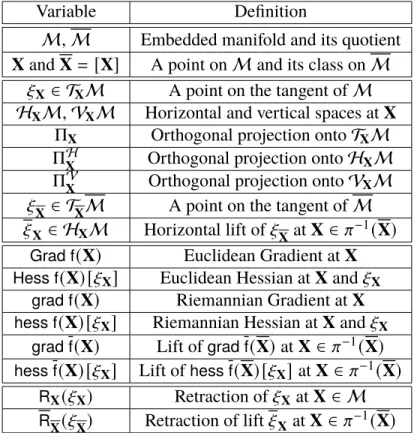
Xt αt ξt X R_Xt(αtξt X) Xt+1 Xt +T_XtM M ExpXt(αtξt X)

Figure 2.1: The update step for the two-dimensional sphere embedded in_R3.

Euclidean to Riemannian spaces. This part explains the general concept of designing optimization algorithms using Riemannian geometry.

The fundamental idea of optimization algorithms on manifolds is to locally ap-proximate the manifold by a linear space known as thetangent space. Afterwards, unconstrained optimization is performed on that tangent space. In particular, a de-scent direction is computed by deriving theRiemannian gradient. Finally, the point on the tangent space is “projected" to the manifold using aretraction. The steps of the algorithm are available in Algorithm 2.1 and an illustration of one iteration of the algorithm is given in Figure 2.1.

Algorithm 2.1Template of optimization algorithms on Riemannian manifolds. Require: ManifoldM, functionf, and retractionR.

1: InitializeX∈ M.

2: while ||grad f(X) ||_X ≥ 𝜖 do

3: Choose search direction𝜉_X ∈ T_XM.

4: Compute step size𝛼.

5: RetractX=RX(𝛼𝜉_X).

6: end while

7: OutputX.

Sections 2.2 and 2.3 define the above relevant concepts from differential and Rie-mannian geometry for embedded and quotient manifolds, respectively. These geo-metric operators are exploited afterwards in Section 2.4 to design various first and second-order optimization algorithms.

(27)

γ1(t) _M γ2(t) X γ₁0(0) γ₂0(0) X+T_XM

Figure 2.2: Tangent space of a 2-dimensional manifold embedded in_R3.

2.2 Embedded Riemannian Manifolds First-Order Embedded Manifolds Geometry

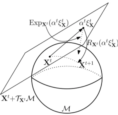
Along the lines of approximating a function locally by its derivatives, a manifoldM of dimension𝑑can be approximated locally at a pointXby a𝑑-dimensional vector spaceTXM generated by taking derivatives of all smooth curves going throughX at the origin. Formally, let𝛾(𝑡) :I ⊂_R→ Mbe a curve onM with𝛾(0)=Xand denote by𝛾0(0)its derivative at 0. The space generated by all such𝛾0(0)represents a vector spaceT_XM called the tangent space ofMatX. Figure 2.2 shows an example of a two-dimensional tangent space generated by a couple of curves. The tangent space plays a primordial role in Riemannian optimization algorithms in the same way that derivatives of functions play an important role in Euclidean optimization. The union of all tangent spacesT Mis referred to as the tangent bundle ofM, i.e.,:

T M = Ø

X∈M

T_XM.

To optimize functions on manifolds, besides the notion of a tangent space described above, one needs the notion of directions and lengths which can be achieved by endowing each tangent spaceTXMby an inner producth𝜉_X, 𝜂_Xi_X, ∀𝜉_X, 𝜂_X ∈ T_XM. Such metric, known as the Riemannian metric, turns the manifold into a Riemannian manifold. The norm on the tangent spaceT_XM is denoted by||.||_X and defined by:

||𝜉_X||_X =

p

h𝜉_X, 𝜉_Xi_X, ∀𝜉_X ∈ T_XM.

Since both the ambient space and the tangent space are vector spaces, one can define the orthogonal projectionΠX :E → TXMverifyingΠX◦ΠX = ΠX. The projection is said to be orthogonal with respect to the restriction of the Riemannian metric to the tangent space, i.e., ΠX is orthogonal in the h., .i_X sense which means that hΠX(Y),Y−Π_X(Y)i_X =0, ∀Y∈ E.

(28)

The Riemannian gradient is defined in a similar manner as the Euclidean one with the exception that it uses the Riemannian geometry, i.e.,:

Definition 2.1 The Riemannian gradient of f of a manifold M at X, denoted by

grad f(X), is defined as the unique tangent vector inT_XMthat satisfies: hgrad f(X), 𝜉_Xi_X =D f(X) [𝜉_X], ∀𝜉_X ∈ T_XM.

While the update stepX𝑡+1 =X𝑡

+𝛼𝑡𝑝𝑡 is trivial in Euclidean optimization thanks to its vector space structure, it might result in a point X𝑡+1

outside the manifold. Moving in a given tangent direction while remaining on the manifold is realized by the retraction operator. The ideal retraction is the exponential map1Exp_Xas it maps a tangent vector 𝜉_X ∈ T_XM to a point on the manifold along the geodesic curve (straight line on the manifold) that goes throughXin the direction of𝜉X. However, computing geodesic curves is challenging and may be more difficult that solving the original optimization problem. Luckily, one can use a first-order approxima-tion of the exponential map, called a retracapproxima-tion herein, without compromising the convergence properties of the algorithms.

Definition 2.2 A retraction on a manifold M is a smooth mapRfrom the tangent

bundleT M ontoM. For allX ∈ M, the restriction ofRtoTXM, denoted byRX, satisfies the following properties:

• Centering: RX(0) =X. • Local rigidity: The curve 𝛾_𝜉

X(𝜏) = RX(𝜏 𝜉X) satisfy 𝛾¤𝜉_X(0) = 𝜉X, ∀ 𝜉X ∈

T_XM.

Embedded Submanifolds: Second-Order Geometry

Generalizing Newton’s method to the Riemannian setting requires computing the Riemannian Hessian which can be accomplished by taking a directional derivative of a vector field. As vectors belong to different tangent spaces, one needs the notion of a connection∇, also called the covariant derivative, which generalizes the notion of directional derivative to vector fields. The definition of a connection is given below:

1_{The exponential map and geodesics are introduced later as part of the second-order geometry}

(29)

Definition 2.3 An affine connection∇is a map that associate to (𝜂, 𝜉) the tangent vector∇𝜂𝜉satisfying for all𝜂, 𝜉 , 𝜒 ∈ T M, for all smoothf,g:M →R, and for all

reals𝑎, 𝑏 ∈_R:

• ∇_f₍𝜂)+g(𝜒)𝜉 =f(∇𝜂𝜉) +g(∇𝜒𝜉)

• ∇𝜂(𝑎 𝜉+𝑏 𝜑) =𝑎∇𝜂𝜉+𝑏∇𝜂𝜑

• ∇𝜂(f(𝜉))=𝜉(𝑓)𝜂+f(∇𝜂𝜉),

wherein the vector field𝜉 acts on the functionfby derivation, i.e.,𝜉(𝑓) =D(f) [𝜉] also noted as𝜉 𝑓 in the literature.

On a Riemannian manifold, the Levi-Civita connection is the canonical choice of affine connections as it preserves the Riemannian metric. Indeed, the Levi-Civita connection is the unique affine connection onM with the Riemannian metrich., .i that satisfies for all𝜂, 𝜉 , 𝜒 ∈ T M:

1. ∇𝜂𝜉− ∇𝜉𝜂= [𝜂, 𝜉]

2. 𝜒h𝜂, 𝜉i= h∇_𝜒𝜂, 𝜉i + h𝜂,∇_𝜒𝜉i,

where [𝜉 , 𝜂] is the Lie bracket, i.e., a function from the set of smooth function to itself defined by [𝜉 , 𝜂]g=𝜉(𝜂(g)) −𝜂(𝜉(g)).

Definition 2.4 The Riemannian Hessian of f at X, denoted by hess f(X), of a manifoldM is a map fromTXM into itself defined by:

hess f(X) [𝜉_X] =∇_𝜉

Xgrad f(X), ∀𝜉X ∈ TXM,

where grad f(X) is the Riemannian gradient and ∇ is the Riemannian connection onM.

Given a Riemannian connection ∇ on M and an interval I ⊆ _R containing 0, a geodesic curve𝛾 :I → M going throughX ∈ M in the direction𝜉_X ∈ T_XM, i.e., 𝛾(0) =Xand𝛾¤(0) =𝜉X, is denoted by𝛾_X_,𝜉

X(𝑡). The geodesic𝛾X,𝜉_X(𝑡) defines the

Exponential map Exp_X : TXM → Mby ExpX(𝜉X) =𝛾_X_,𝜉

X(1). In addition, if there

exists a unique geodesic𝛾_X_,𝜉

X(𝑡) between the pointsXand𝛾X,𝜉_X(1) =Y∈ M, the

(30)

Log_X(Y) =Exp−_X1(Y) =𝜉X. Under the previous assumption, the geodesic distance on M, i.e., shortest distance, between points X and Y is defined and denoted by 𝑑(X,Y) =||Log_X(Y) ||_X = ||Log_Y(X) ||_Y. Given two pointsXandYinM and the geodesic 𝛾_X_,𝜉

X(1) = Y, the parallel translation Γ

Y

X : TXM → TYM of the tangent vector𝜂∈ T_XM is denoted byΓY

X𝜂 ∈ TYM. 2.3 Quotient Riemannian Manifolds

Equivalence Relationship and Quotient Structure

Let∼be an equivalence relationship and define the setM =M/∼as the quotient of the manifoldM by∼. In order to show that the setM𝑛𝑝 =M

𝑛

𝑝/∼admits a manifold

structure, it is sufficient to show that∼is regular [23], meaning that it satisfies the three following properties

1. graph(∼)is an embedded submanifold of the productM𝑛 𝑝× M

𝑛 𝑝.

2. The projection𝜋₁:graph (∼) → M𝑛

𝑝given by𝜋1(X1,X2) =X1is a submer-sion. 3. graph(∼) is closed, whereingraph (∼) ={(X1,X₂) ∈ M𝑛 𝑝× M 𝑛 𝑝 |X1∼ X2}.

Combining the three properties above allows concluding thatM𝑛𝑝admits a unique

manifold structure known as the quotient manifold ofM𝑛

𝑝by∼. However, it does not

allow to conclude thatM𝑛𝑝 inherits the Riemannian structure ofM 𝑛

𝑝 as it requires

the Riemannian metric to be compatible with∼, as described in the next part. Under the above assumptions, the quotient manifoldM admits a quotient structure that groups all elements ofM in the same equivalence class as a single point. Let 𝜋 be the natural projection that associates to each X ∈ M its equivalence class 𝜋(X) = [X] = X ∈ M. These three notations for equivalence classes are used interchangeably in this paper.

Quotient Submanifolds: First-Order Geometry

Let h., .i_X be the Riemannian metric on the tangent space T_XM of the embedding spaceM. The quotientM =M/∼admits a Riemmanian structure for the induced Riemannian metric if and only if the metric is compatible with the equivalence relationship∼, i.e., it does not depend on the chosen representative of the equivalence class.

(31)

To express the compatibility of the metric, we first introduce the horizontal lift. For a pointX∈ M, let 𝜉

X ∈ TXM be a tangent vector. In a similar manner thatXcan be represented by multiple X ∈ 𝜋−1(X), the tangent vector𝜉

X can be represented by multiple predecessors for eachX ∈ 𝜋−1(X). Indeed, fixX ∈ 𝜋−1(X), then any tangent vector 𝜉_X ∈ T_XM satisfying D (𝜋(X)) [𝜉_X] = 𝜉

X can be considered as a valid representation of the tangent vector 𝜉

X. To circumvent the aforementioned problem and obtain a unique representation of𝜉

X for each predecessorX∈𝜋

−1₍_X₎_,

we use the fact that 𝜋−1(X) represents a manifold. Therefore, one can obtain a unique representation by orthogonally decomposing the tangent spaceT_XM into a vertical spaceV_XMand a horizontal spaceH_XM such that

V_XM =T_X𝜋−1(X) T_XM =V_XM ⊕ H_XM.

The ambient vector space can be composed into a tangent space T_XM and its orthogonal complement T_X⊥M. In particular, for each X ∈ M, the embedding space _R𝑛×𝑚

can be uniquely decomposed into a direct sum of the above defined linear space, i.e.,

R𝑛×𝑚 =HXM ⊕ VXM ⊕ T_X⊥M.

The representation of𝜉

X ∈ TXM atX ∈ 𝜋

−1₍_X₎_{, denoted by}_𝜉

X and referred to as the horizontal lift of a tangent vector𝜉

XatX, is the unique element in the horizontal spaceH_XM satisfyingD(𝜋(X)) [𝜉_X] = 𝜉

X. Such representation as horizontal lift allows to get a unique parameterization of tangent vectors in a quotient manifold. The manifold M represents a Riemannian manifold for the Riemmanian metric h., .i

X on TXM if and only if for all tangent vectors 𝜉X, 𝜂X ∈ TXM the following holds

h𝜉

X1, 𝜂X1iX1 =h𝜉X2, 𝜂X2iX2, ∀X1,X2∈ 𝜋

−1₍_X₎_.

Under the above assumption, the operator h., .i

X on TXM defined by h𝜉X, 𝜉XiX = h𝜉_X, 𝜂_Xi_X for anyX∈ 𝜋−1(X) represents a well-defined Riemannian metric for the quotient manifoldM. LetΠ_XH be the orthogonal projection from the ambient space

R𝑛×𝑚 to the horizontal spaceHXMand letf:M →Rbe a function that is constant

on each equivalence class [X] for all X ∈ M. The above function, said to be compatible with the equivalence relationship, induces a functionf :M → _Rsuch

(32)

thatf(X) =f(X)for any predecessorXof the equivalence classX. Under the above assumptions, the Riemannian gradient is obtained by projecting the Euclidean one onto the horizontal space of any predecessor, i.e.,

grad f(X) = ΠH_X (Grad f(X)), X∈ 𝜋−1(X).

Second-Order Geometry of Quotient Manifolds

In the same manner as for the embedded manifold, the Riemannian Hessian can be expressed as the covariant derivative of the Riemannian gradient on the quotient manifold hess f(X) [𝜉

X] = ∇𝜉_Xgrad f(X). Given that the ambient space, R 𝑛×𝑚

herein, is a vector space and that the Riemannian metric is induced and compatible, the connection simplifies as∇𝜉

X𝜂X = Π

H

X (D(𝜂X) [𝜉X]), for anyX ∈𝜋−1(X)which allows the Riemannian Hessian to be expressed as

hess f(X) [𝜉

X] = Π

H

X (D(grad f(X)) [𝜉X]).

LetX∈ MandX1andX2be any twoarbitraryrepresentatives in𝜋−1(X). Assume that the retractions RX1 and RX2 on the tangent spaces TX1M and TX2M of the

manifoldMsatisfy the property𝜋(R_X

1(𝜉X1))=𝜋(RX2(𝜉X2))for all tangent vectors.

Such retraction is said to be compatible with the equivalence relationship and generate a retraction on the quotient manifold as follow

R_X(𝜉

X) =𝜋(RX(𝜉X)),X∈ 𝜋

−1₍_X₎_. _(2.4)

2.4 Optimization on Riemannian Manifolds

This part exploits the geometry operators introduced in the previous sections to design Riemannian optimization algorithms. In particular, the paper illustrates the a generalization of the Riemannian steepest-descent algorithm, known as line-search algorithms. Afterward, a second-order algorithm is presented in the form of the Rie-mannian version of Newton’s method. Finally, a more-sophisticated algorithm, i.e., conjugate gradient, is introduced. Although this manuscript considers sophisticated second-order algorithms on Riemannian manifolds, such as the trust-region (TR) method, these methods can be derived using the geometry operators introduced in this manuscript and are omitted herein. Nonetheless, their performance is reported in each corresponding simulation section.

Line-Search Algorithms on Manifolds

The Riemannian version of the steepest-descent follows similar steps as the Eu-clidean one with the exception that the search direction is obtained with respect

(33)

to the Riemannian gradient. After choosing the search direction as mandated by (2.1), the step size is selected according to Wolfe’s conditions using the backtracking procedure. As stated earlier, the update stepX𝑡+1

=X𝑡

+𝛼𝑡𝑝𝑡 is trivial in Euclidean optimization thanks to its vector space structure. However, it might result in a point X𝑡+1

outside the manifold which motivates the use of retractions. The ideal retrac-tion is the exponential map Exp_X as it maps a tangent vector𝜉_X ∈ T_XM to a point on the manifold along the geodesic curve (straight line on the manifold) that goes throughXin the direction of𝜉X. However, the convergence of the steepest-descent algorithm is guaranteed under the use of a first-order retraction. Therefore, the gen-eralization of the steepest-descent algorithm to Riemannian manifolds is obtained by finding the search direction that satisfies equation (2.2) for the Riemannian metric. The update is, then, mapped to the manifold using the retraction. The steps of the method are summarized in Algorithm 2.2.

Algorithm 2.2 Template of the gradient descent procedure on Riemannian mani-folds.

Require: ManifoldM, functionf, and retractionR.

2: while ||grad f(X) ||X ≥ 𝜖 do

3: Choose search direction𝜉_X ∈ T_XM such that: hgrad f(X), 𝜉_Xi_X < 0.

4: Compute Armijo step size𝛼using backtracking.

5: RetractX=RX(𝛼𝜉_X).

6: end while

7: OutputX.

Newton’s Method on Riemannian Manifolds

Algorithm 2.3Template of Newton’s method on Riemannian manifolds. Require: ManifoldM, functionf, retractionR, and affine connection∇.

2: while ||grad f(X) ||_X ≥ 𝜖 do

3: Find descent direction𝜉_X ∈ T_XM such that:

hess f(X) [𝜉_X] =−grad f(X), whereinhess f(X) [𝜉_X] =∇_𝜉 Xgrad f(X) 4: RetractX=RX(𝜉_X). 5: end while 6: OutputX.

(34)

Given the above definitions, the generalization of Newton’s method to Riemannian manifolds is accomplished by replacing both the Euclidean gradient and Hessian by their Riemannian counterparts in (2.3). Hence, the search direction is the tangent vector 𝜉_X that satisfies hess f(X) [𝜉_X] = −grad f(X). The update is obtained by retracting the tangent vector to the manifold similar to the steepest-descent algorithm. The full steps of the algorithm are illustrated in Algorithm 2.3.

Riemannian Conjugate Gradient Algorithm

Algorithm 2.4 Template of the conjugate gradient method on Riemannian mani-folds.

Require: ManifoldM, functionf, retractionR, and vector transportT.

2: InitializeY=−grad f(X).

3: while ||grad f(X) ||X ≥ 𝜖 do

4: Compute step size𝛼using line-search procedures, e.g., backtracking.

5: RetractX=RX(𝛼Y).

6: Compute 𝛽using (2.7), (2.8), or (2.9).

7: UpdateY=−grad f(X) +𝛽T𝛼_Y(Y).

8: end while

9: OutputX.

The conjugate gradient algorithm is an unconstrained optimization method devel-oped for solving quadratic equations of the form

min x∈R𝑛 1 2x T_Ax₋_xT_b ,

wherein matrix A is an 𝑛 × 𝑛 symmetric positive-definite matrix and b ∈ _R𝑛. While simple first-order algorithms fail to converge quickly for problems with ill-conditioned matrix A, the conjugate gradient method alleviates the problem by choosing only conjugate search directions in which the inner product is computed with respect to the matrix A. Therefore, the main idea of conjugate gradient algorithms is to perform the update

x𝑘+1 =x𝑘+𝛼𝑘p𝑘, (2.5)

whereinp𝑡 𝑘

𝑡=1are conjugate directions related thought the expression

p𝑘+1= 𝛽𝑘p𝑘−Grad f(x𝑘), (2.6)

with𝛽_𝑘can be chosen independently, yielding different nonlinear conjugate gradient methods.

(35)

The generalization of the conjugate gradient from Euclidean spaces to Rieman-nian manifolds is not direct. Indeed, unlike the RiemanRieman-nian steepest-descent, the conjugate gradient algorithm cannot be readily extended to Riemannian manifolds as equation (2.6) combines different gradients which is not possible on manifolds. Indeed, each Riemannian gradient lives in a different tangent space. This issue is resolved throught the concept of parallel translation to connect different tangent spaces in a manifold. However, similar to the use of a retraction instead of the complicated Exponential map, one can use a vector transport instead of the more difficult to derive parallel translation. A vector transport Tcan be obtained by ex-ploiting the linear structure of the embedding space and the notion of retraction as

T𝜂_Y(𝜉_Y) = Π_R

Y(𝜂_Y)(𝜉Y)(see Proposition 8.1.2 [23]).

The Riemannian version of the conjugate gradient can be described as follows. Starting from an initial guessX0, the initial residue is computed asY0=−grad f(X0).

Afterward, while not converged, the step size 𝛼_𝑘 is computed using line-search procedures, e.g., backtracking. Generalizing the linear combination in (2.5) gives the update via the retractionX𝑘+1 =RX𝑘(

𝛼_𝑘Y_𝑘). Finally, the residue is updated as Y𝑘+1=−grad f(X𝑘+1) +𝛽𝑘+1T𝛼𝑘Y𝑘(Y𝑘), where the𝛽𝑘+1can be one of the following

choices

• Quasi Newton [23]

𝛽_𝑘₊₁=

hT𝛼𝑘Y𝑘(Y𝑘),Hess f(X𝑘) [grad f(X𝑘)]iX𝑘

hT𝛼𝑘Y𝑘(Y𝑘),Hess f(X𝑘) [T𝛼𝑘Y𝑘(Y𝑘)]iX𝑘 . (2.7) • Fletcher-Reeves [72]: 𝛽_𝑘₊₁= hgrad f(X𝑘+1),grad f(X𝑘+1)iX𝑘+₁ hgrad f(X𝑘),grad f(X𝑘)iX𝑘 . (2.8) • Polak-Ribiere [73]: 𝛽_𝑘₊₁=

hgrad f(X𝑘+1),grad f(X𝑘+1) −T𝛼𝑘Y𝑘(grad f(X𝑘)iX𝑘+₁

hgrad f(X𝑘),grad f(X𝑘)iX𝑘

. (2.9)

Finally, after obtaining the 𝛽_𝑘₊₁, the residue is updated through the equation Y𝑘+1 = −grad f(X𝑘) + 𝛽𝑘+1T𝛼Y𝑘(Y𝑘). The steps of the algorithm are summarized

(36)

C h a p t e r 3

EFFICIENT RIEMANNIAN ALGORITHMS FOR COMMUNITY

DETECTION

[1] A. Douik and B. Hassibi. “A Riemannian Approach for Graph-Based Clus-tering by Doubly Stochastic Matrices”. In: Proc. of the IEEE Statistical Signal Processing Workshop (SSP’ 2018), Freiburg, Germany. Vol. 1. 1. June 2018, pp. 806–810. doi:10.1109/SSP.2018.8450685.

[2] A. Douik and B. Hassibi. “Manifold Optimization Over the Set of Doubly Stochastic Matrices: A Second-Order Geometry”. In:IEEE Transactions on Signal Processing67.22 (Nov. 2019), pp. 5761–5774. doi:10.1109/TSP. 2019.2946024.

This chapter suggests using a Riemannian optimization approach to solve a subset of convex optimization problems wherein the optimization variable is a doubly stochastic matrix. Optimization over the set of doubly stochastic matrices is crucial for multiple communications and signal processing applications, especially graph-based clustering. The paper introduces and investigates the geometries of three convex manifolds, namely the doubly stochastic, the symmetric, and the definite multinomial manifolds which generalize the simplex, also known as the multinomial manifold. Theoretical complexity analysis and numerical simulation results testify the efficiency of the proposed method over state-of-the-art algorithms for clustering applications. In particular, they reveal that the proposed framework outperforms conventional generic and specialized approaches, especially in high dimensions. The results on this chapter appear in the research papers [74] and [75] and as such some of the text appears as it is in these publications.

3.1 Clustering via Optimization over the Set of Doubly Stochastic Matrices State-of-the-Art Clustering Approaches

Optimization over the set of doubly stochastic matrices is a particularly interesting class of problems for its connection with probability density functions and its numer-ous applications in communications and signal processing, especially in graph-based clustering [39, 53, 54, 55]. Furthermore, doubly stochastic matrices play an impor-tant role in graph theory such as in critical arcs for strongly connected graphs [76] and in optimizing the mixing time of Markov chains with applications in network