Address: IIASA, Schlossplatz 1, A-2361 Laxenburg, Austria
Email: [email protected] Department: Advanced Systems Analysis | ASA
Risk and Resilience | RISK
Working paper
Economic Forecasting with an Agent-based
Model
Sebastian Poledna ([email protected])
Michael Gregor Miess ([email protected]) Cars Hommes ([email protected])
WP-20-001
Name Elena Rovenskaya
Program: Program Director Advanced Systems Analysis; Acting Program Director Evolution and Ecology Date: 17 January 2020
Table of contents
Abstract……….3
Acknowledgments………4
Introduction……….5
Related literature………..6
An agent-based model for a small open economy………...7
Forecast performance……….…10
Conclusion……….…18
References………19
Appendix A Details of the agent-based model …….………..22
Appendix B Parameters for the Austrian economy……….………..36
Appendix C Initial conditions for the Austrian economy……….43
Appendix D Conditional forecasts with the agent-based model……….………...46
Appendix E Macroeconomic variables……….……...47
Appendix F DSGE model used for out-of-sample-prediction………...48
ZVR 524808900
This research was funded by IIASA and its National Member Organizations in Africa, the Americas, Asia, and Europe. Michael Miess additionally acknowledges funding from IIASA through the Systems Analysis Forum Project “A big-data approach to systemic risk in very large financial networks”, the Austrian Research Promotion Agency FFG under grant number 857136, and from the Austrian Central Bank (Osterreichische Nationalbank, OeNB) Anniversary Fund (Jubiläumsfonds) under grant number 17400. Sebastian Poledna additionally acknowledges funding from a research fellowship at the Institute for Advanced Study of the University of Amsterdam.
This work is licensed under a Creative Commons Attribution-NonCommercial 4.0 International License. For any commercial use please contact [email protected]
Working Paperson work of the International Institute for Applied Systems Analysis receive only limited review. Views or opinions expressed herein do not necessarily represent those of the institute, its National Member Organizations, or other organizations supporting the work.
Abstract
We develop the first agent-based model (ABM) that can compete with benchmark VAR and DSGE models in out-of-sample forecasting of macro variables. Our ABM for a small open economy uses micro and macro data from national and sector accounts, input-output tables, government statistics, census and business demography data. The model incorporates all economic activities as classified by the European System of Accounts as heterogeneous agents. The detailed structure of the ABM allows for a breakdown into sector level forecasts. Potential applications of the model include stress-testing and predicting the effects of changes in monetary, fiscal, or other macroeconomic policies.
About the authors
Sebastian Poledna is a Research Scholar in the Advanced Systems Analysis (ASA) and Risk and Resilience (RISK) programs at IIASA. He was a research fellow at the Institute for Advanced Study of the University of Amsterdam and a Visiting researcher at the Earthquake Research Institute of the University of Tokyo. Sebastian Poledna developed, implemented and estimated the model and performed the simulations. He gathered and processed the data for the model, analyzed simulation results, and wrote the manuscript as well as the Appendix on the ABM. (Contact: [email protected])
Michael Gregor Miess is a Research Associate at the Institute for Ecological Economics at the Vienna University of Economics and Business (WU Wien), and a Researcher in the group Macroeconomics and Economic Policy at the Institute for Advanced Studies in Vienna (IHS). He was a Research Assistant in the Advanced Systems Analysis (ASA) and Risk and Resilience (RISK) programs at IIASA, and a pre-doctoral researcher at the Complexity Science Hub Vienna. Michael Gregor Miess gathered and processed the data for the model. He analyzed simulation results and wrote the manuscript as well as the Appendices on the ABM and the DSGE model. (Contact: [email protected])
Cars Hommes is the Director of CeNDEF at the University of Amsterdam, a Research Fellow of the Tinbergen Institute, and a Senior Research Advisor of the Bank of Canada. Cars Hommes analyzed simulation results and wrote the manuscript. (Contact: [email protected])
Acknowledgments
We are grateful for the inspiration and vision from J. Doyne Farmer. We would like to thank the following people: Jakob Grazzini for providing us with the code of the model developed in Assenza et al. (2015); Katrin Rabitsch for providing us with the codes of an improved version of the DSGE model developed in Breuss and Rabitsch (2009), and for her advice and assistance; Tolga Özden for his help with the estimation of the DSGE model; Stefan Thurner for his participation in early discussions in the initiation of the ideas incorporated and reported in the manuscript; researchers at the Institute for Advanced Studies Vienna and at CeNDEF; as well as conference and seminar participants and discussants at the International Conference on Computing in Economics and Finance (CEF) 2017 and 2018, the Second Conference on Network Models and stress testing for financial stability at Banco de México 2017, the 11th Workshop on Economic Complexity at the SKEMA Business 2017, the 1st Vienna Workshop on Economic Forecasting 2018 at IHS, the March 2018 DNB Lunchseminar at the De Nederlandsche Bank; and, in particular, Jesus Crespo Cuaresma, Cees Diks, Marco van der Leij, Mauro Napoletano, Helmut Hofer, Michael Reiter, and Leopold Sögner for stimulating discussions and valuable comments.
1 Introduction
The dominant theory-driven approach to modeling the economy over recent decades has been the dynamic stochastic general equilibrium (DSGE) model. In particular, models following the New Keynesian paradigm, that include financial and real frictions to replicate phenomena observed in empirical data, have become a new standard in macroeconomics (Christiano et al.,2010;Brunnermeier et al.,2013). Together with structural econometric and vector autoregressive (VAR) models of various types and sizes, DSGE models are the workhorse framework of central banks and other institutions engaging in economic forecasting, especially since the advent of Bayesian DSGE models such asSmets and Wouters(2003,2007), exhibiting good forecasting capabilities when compared to simple time series models. One of the main reasons for the evident success of DSGE models is their rigorous micro-foundations rooted in economic theory, which have been complemented by Bayesian parameter estimation techniques to reach a better empirical fit (An and Schorfheide,2007;Fernandez-Villaverde, 2010;Linde et al.,2016). However, in the light of the financial crisis of 2007-2008 and the subsequent Great Recession, these models have been criticized by several prominent voices within the economic profession, coming from different schools of economic thought. The limits of the DSGE approach at the core of the New Neoclassical Synthesis have been discussed in detail, for example, in (Vines and Wills,2018).1 As an alternative, some economists are pushing forward with agent-based models (ABMs)—potentially to complement DSGE models—as a new promising direction for economic modelling.2 Farmer and Foley(2009), in particular, suggest that it might be possible to conduct economic forecasts with a macroeconomic ABM, although they consider this to be ambitious.
ABMs have two distinguishing features: they are “agent-based,” that is, they model individual agents— households, firms, banks, etc.—and they aresimulation modelsbecause they are too detailed and complex to be handled analytically. The dynamic properties of the aggregate system are derived “from the bottom up,” namely, they emerge from the micro-behavior of individual agents and the structure of their interactions. Macroeconomic ABMs typically replicate a number of macroeconomic and microeconomic empirical stylized facts, such as time series properties of output fluctuations and growth, as well as cross-sectional distributional characteristics of firms (Dosi et al.,2017;Axtell,2018). Macroeconomic ABMs relax two key assumptions at the core of the New Neoclassical Synthesis—the single, representative agent and the rational, or model-consistent, expectations hypothesis (Haldane and Turrell,2018). Representative agents are replaced by individual “agents” who follow well-defined behavioral rules of thumb, and rational expectations are relaxed to bounded rationality (i.e., agents make decisions based on partial information and limited computational ability). Relaxation of these assumptions allows greater flexibility in the design of ABMs because the strong consistency requirements entailed in simplistic models—all actions and beliefs must be mutually consistent at all times—are no longer necessary. ABMs occupy a middle ground on a spectrum where micro-founded DSGE models lie at one end and statistical models lie at the other (Haldane and Turrell,2018).3,4 Macroeconomic ABMs, however, suffer from a number of problems that impede major applications in economics, such as economic forecasting and empirically founded policy evaluation. The lack of a commonly accepted basis for the modeling of bounded rational behavior has raised concerns about the “wilderness of bounded rationality” (Sims,1980). Research on econometric estimation of ABMs has been growing recently, though most of it still remains at the level of proof of concept (Lux and Zwinkels, 2018). Empirical validation of ABMs remains a difficult task. Due to over-parameterization and the corresponding degrees of freedom, almost any simulation output can be generated with an ABM, and thus replication of stylized facts only represents a weak test for the validity of ABMs (Fagiolo and Roventini,2017).
The main goal of this paper is to develop an ABM that fits microeconomic data of a small open economy and allows out-of-sample forecasting of the aggregate macro variables, such as GDP (including its components), inflation and interest rates.5 The model is based onAssenza et al.(2015) who developed a stylized ABM with households, firms (upstream and downstream), and a bank, that replicates a number of stylized facts. Our ABM includes all institutional sectors (financial firms, non-financial firms, households, and a general government), where the firm sector is composed of 64 industry sectors according to national accounting conventions and the structure of input-output tables. The model is based on micro and macro data from national accounts,
1For earlier critiques see e.g.,Canova and Sala(2009),Colander et al.(2009),Kirman(2010),Krugman(2011),Stiglitz(2011,2018),
Blanchard(2016),Romer(2016). See also the recent response defending DSGE models byChristiano et al.(2018).
2Some examples includeFreeman(1998),Gintis(2007),Colander et al.(2008),LeBaron and Tesfatsion(2008),Farmer and Foley(2009),
Trichet(2010),Stiglitz and Gallegati(2011), andHaldane and Turrell(2018).
3There is also a large literature on DSGE models with heterogeneous agents that maintains the rational expectations hypothesis. See e.g., the collection of chapters inSchmedders and Judd(2013).
4In recent years another large literature has appeared on behavioral macro-models with boundedly rational agents and heterogeneous expectations. See the recent overview inHommes(2018).
5A related model that does not allow out-of-sample forecasting of macro variables was used for estimating indirect economic losses from natural disasters in (Poledna et al.,2018).
sector accounts, input-output tables, government statistics, census data, and business demography data. Model parameters are either taken directly from data or calculated from national accounting identities. For exogenous processes such as imports and exports, parameters are estimated. The model furthermore incorporates all economic activities, as classified by the European System of Accounts (ESA) (productive and distributive transactions) and all economic entities; namely, all juridical and natural persons are represented by heterogenous agents. The model includes a complete GDP identity, where GDP as a macroeconomic aggregate is calculated from the market value of all final goods and services produced by individual agents and market value emerges from trading or, alternatively, according to the aggregate expenditure or income of individual agents. Markets are fully decentralized and characterized by a continuous search-and-matching process, which allows for trade frictions. Agent forecasting behavior is modeled by parameter-free adaptive learning, where agents act as econometricians who estimate the parameters of their model and make forecasts using their estimates (Evans and Honkapohja,2001). We follow the approach ofHommes and Zhu(2014), where agents learn the optimal parameters of simple parsimonious AR(1) rules in a complex environment6.
The objectives of this paper are twofold. First, we develop the first ABM that fits the microeconomic data of a small open economy and allows out-of-sample forecasting of the aggregate macro variables, such as GDP (including its components), inflation and interest rates. Second, as an empirical validation, we compare the forecast performance of the ABM to that of autoregressive (AR), VAR, and DSGE models. For this purpose, we conduct a series of forecasting exercises where we evaluate the out-of-sample forecast performance of the different model types using a traditional measure of forecast error (root mean squared error). In a first exercise, we validate the ABM against unconstrained VAR models that are estimated on the same dataset as the ABM. We find that the ABM delivers a similar forecast performance to the VAR model for short- to medium-term horizons up to two years, and improves on VAR forecasts for longer horizons up to three years. In a second exercise, we compare the forecast performance of the ABM to that of AR models and a standard DSGE model for the main macroeconomic aggregates, GDP growth and inflation, as well as to household consumption and investment as main components of GDP. For a DSGE model, we have employed the standard DSGE model of Smets and Wouters(2007), adapted to the Austrian economy byBreuss and Rabitsch(2009). Here, we find that the ABM delivers a similar forecast performance to that of the standard DSGE model. Both the ABM and the standard DSGE model improve on the AR models in forecasting household consumption and investment. In a third forecasting setup, we generate forecasts conditional on exogenous paths for imports, exports, and government consumption, corresponding to a small open economy setting and exogenous policy decisions. In this forecast exercise, the detailed economic structure incorporated into the ABM improves its forecasting ability, especially in comparison with the DSGE model. We perform two more forecasting exercises exploring the detailed sectoral structure of our ABM. With these three forecast exercises, we achieve comparability of the ABM to the forecasting performance of standard modeling approaches. To the best of our knowledge, this is the first ABM able to compete in out-of-sample forecasting of macro variables.
The remainder of the manuscript is structured as follows. Section2elaborates on the characteristics of ABMs, and critiques of them, and gives a brief summary of the related literature. Section3provides an overview of the model describing agents’ behavior and the data used. Section4describes the forecast performance of the ABM, where we validate the ABM against VAR, DSGE, and AR models in different forecasting setups, and delivers applications to more detailed decompositions of the ABM forecasts. Section5concludes. The details of our ABM are given in AppendicesAtoC.
2 Related literature
Since their beginnings in the 1930s,7 ABMs have found widespread application as an established method in various scientific disciplines (Haldane and Turrell,2018), for example, military planning, the physical sciences, operational research, biology, ecology, but less so in economics and finance. The use of ABMs in the latter two fields to date remains quite limited in comparison to other disciplines. An early exception isOrcutt(1957), who constructed a first simple economically motivated ABM to obtain aggregate relationships from the interaction of individual heterogeneous units via simulation. Other examples include topics such as racial segregation patterns
6Brayton et al.(1997) discuss the role of expectations in FRB/US macroeconomic models. One approach is that expectations are given by small forecasting models such as a VAR model. Our choice of AR(1) models is simply the most parsimonious yet empirically relevant choice, where, for each relevant variable, agents learn the parameters of an AR(1) rule consistent with the observable sample mean and autocorrelation.Slobodyan and Wouters(2012) estimated theSmets and Wouters(2007) DSGE model with expectations modelled by a simple AR(2) forecasting rule under time-varying beliefs and show that this leads to an improvement in the empirical fit of the model and its ability to capture the short-term momentum in the macroeconomic variables.Hommes et al.(2019) estimate the benchmark 3 equations New Keynesian model with optimal AR(1) rules for inflation and output gap and find a better fit than under rational expectations.
(Schelling,1969), financial markets (Arthur et al.,1997), or more recently the housing market (Geanakoplos et al., 2012;Baptista et al.,2016). Since the financial crisis of 2007–2008, ABMs have increasingly been applied to research in macroeconomics. Furthermore, in recent years, several ABMs have been developed that depict entire national economies and are designed to deliver macroeconomic policy analysis. The European Commission (EC) has in part supported this endeavor. One example of a large research project funded by the EC is the Complexity Research Initiative for Systemic Instabilities (CRISIS),8an open source collaboration between academics, firms, and policymakers (Klimek et al.,2015). Another is EURACE,9a large micro-founded macroeconomic model with regional heterogeneity (Cincotti et al.,2010).
In a recent overviewDawid and Delli Gatti(2018) identified seven main families of macroeconomic ABMs10: (1) the framework developed by Ashraf et al.(2017); (2) the family of models proposed by Delli Gatti et al. (2011) in Ancona and Milan exploiting the notion of Complex Adaptive Trivial Systems (CATS); (3) the framework developed byDawid et al.(2018) in Bielefeld as an offspring of the EURACE project, known as Eurace@Unibi; (4) the EURACE framework maintained byCincotti et al.(2010) in Genoa; (5) the Java Agent based MacroEconomic Laboratory developed bySeppecher et al.(2018); (6) the family of models developed byDosi et al.(2017) in Pisa, known as the “Keynes meeting Schumpeter” framework; and (7) the LAGOM model developed by Jaeger et. al (2013). What unites all these families of models is their ability to generate endogenous long-term growth and short- to medium-term business cycles. These business cycles are the macroeconomic outcome of the micro-level interaction of heterogeneous agents in the economy as a complex system subject to non-linearities (Dawid and Delli Gatti,2018). All these models assume bounded rationality for their agents, and thus suppose adaptive expectation in an environment of fundamental uncertainty. Typically, they minimally depict firm, household, and financial (banking) sectors populated by numerous agents of these types (or classes), and agents exhibit additional heterogeneity within one or more of the different classes. All results are obtained by performing extensive Monte Carlo simulations and averaging over simulation outcomes. The great majority of models are calibrated and validated with respect to a (smaller or larger) variety of stylized empirical economic facts (Fagiolo and Roventini,2017). However, despite their level of sophistication, all these models suffer from one or more impediments: they serve as a theoretical explanatory tool constructed for a hypothetical economy; the choice of the number of agents is arbitrary or left unexplained; time units may have no clear interpretation; validation with respect to stylized empirical facts cannot solve the potential problem of over-parameterization; the choice of parameter values is often not pinned down by clear-cut empirical evidence; and most of these models exhibit an extended transient or burn-in phase that is discarded before analysis.
To address these concerns we develop an ABM that fits microeconomic data of a small open economy and allows out-of-sample forecasting of the aggregate macro variables, such as GDP (including its components), inflation and interest rates. This model is based on micro and macro data from national accounts, input-output tables, government statistics, census data, and business demography data. Model parameters are either taken directly from data or are calculated from national accounting identities. For exogenous processes, such as imports and exports, parameters are estimated. As an empirical validation, we compare the out-of-sample forecast performance of the ABM to that of AR, VAR, and DSGE models.
3 An agent-based model for a small open economy
In this section we give a short overview of the model; for details, see AppendicesAtoC. Following the sectoral accounting conventions of the ESA,Eurostat(2013), the model economy is structured into four mutually exclusive domestic institutional sectors: (1) non-financial corporations (firms); (2) households; (3) the general government; and (4) financial corporations (banks), including (5) the central bank. These four sectors make up the total domestic economy and interact with (6) the rest of the world (RoW) through imports and exports. Each sector is populated by heterogeneous agents, who represent natural persons or legal entities (corporations, government entities, and institutions). We use a scale of 1:1 between model and data, so that each agent in the model represents a natural or legal person in reality. This has the advantage that our ABM is directly linked to microeconomic data and that scaling or fine tuning of parameters and size is not needed; rather, parameters are pinned down by data or calculated from accounting identities. All individual agents have separate balance sheets, depicting assets, liabilities, and ownership structures. The balance sheets of the agents, and the economic flows between them, are set according to data from national accounts.
The firm sector is composed of 64 industry sectors according to the NACE/CPA classification by ESA and the structure of input-output tables. The firm population of each sector is derived from business demography data,
8FP7-ICT grant 288501,http://cordis.europa.eu/project/rcn/101350_en.html. (Last accessed November 30th,2018)
9FP6-STREP grant 035086, http://cordis.europa.eu/project/rcn/79429_en.html. See also: http://www.wiwi. uni-bielefeld.de/lehrbereiche/vwl/etace/Eurace_Unibi/(Last accessed November 30th,2018)
while firm sizes follow a power law distribution, which approximately corresponds to the firm size distribution in Austria. Each firm is part of a certain industry and produces industry-specific output by means of labor, capital, and intermediate inputs from other sectors—employing a fixed coefficient (Leontief) production technology with constant coefficients. These productivity and technology coefficients are calculated directly from input-output tables. Firms are subject to fundamental uncertainty regarding their future sales, market prices, the availability of inputs for production, input costs, and cash flow and financing conditions. Based on partial information about their current status quo and its past development, firms have to form expectations to estimate future demand for their products, their future input costs, and their future profit margin. According to these expectations—which are not necessarily realized in the future—firms set prices and quantities. We assume that firms form these expectations using simple autoregressive time series models (AR(1) expectations). These expectations are parameter-free, as agents learn the optimal AR(1) forecast rule that is consistent with two observable statistics, the sample mean and the sample autocorrelation (Hommes and Zhu,2014). Output is sold to households as consumption goods or investment in dwellings and to other firms as intermediate inputs or investment in capital goods, or it is exported. Firm investment is conducted according to the expected wear and tear on capital. Firms are owned by investors (one investor per firm), who receive part of the profits of the firm as dividend income.
The household sector consists of employed, unemployed, investor, and inactive households, with the respective numbers obtained from census data. Employed households supply labor and earn sector-specific wages. Unemployed households are involuntarily idle, and receive unemployment benefits, which are a fraction of previous wages. Investor households obtain dividend income from firm ownership. Inactive households do not participate in the labor market and receive social benefits provided by the government. Additional social transfers are distributed equally to all households (e.g., child care payments). All households purchase consumption goods and invest in dwellings which they buy from the firm sector. Due to fundamental uncertainty, households also form AR(1) expectations about the future that are not necessarily realized. Specifically, they estimate inflation using an optimal AR(1) model to calculate their expected net disposable income available for consumption.
The main activities of the government sector are consumption on retail markets and the redistribution of income to provide social services and benefits to its citizens. The amount and trend of both government consumption and redistribution are obtained from government statistics. The government collects taxes, distributes social as well as other transfers, and engages in government consumption. Government revenues consist of (1) taxes: on wages (income tax), capital income (income and capital taxes), firm profit income (corporate taxes), household consumption (value-added tax), other products specific, paid by industry sectors), firm production (sector-specific), as well as on exports and capital formation; (2) social security contributions by employees and employers; and (3) other net transfers such as property income, investment grants, operating surplus, and proceeds from government sales and services. Government expenditures are composed of (1) final government consumption; (2) interest payments on government debt; (3) social benefits other than social benefits in kind; (4) subsidies; and (5) other current expenditures. A government deficit adds to its stock of debt, thus increasing interest payments in the periods thereafter.
The banking sector obtains deposits from households as well as from firms, and provides loans to firms. Interest rates are set by a fixed markup on the policy rate, which is determined according to a Taylor rule. Credit creation is limited by minimum capital requirements, and loan extension is conditional on a maximum leverage of the firm, reflecting the bank’s risk assessment of a potential default by its borrower. Bank profits are calculated as the difference between interest payments received on firm loans and deposit interest paid to holders of bank deposits, as well as write-offs due to credit defaults (bad debt). The central bank sets the policy rate based on implicit inflation and growth targets, provides liquidity to the banking system (advances to the bank), and takes deposits from the bank in the form of reserves deposited at the central bank. Furthermore, the central bank purchases external assets (government bonds) and thus acts as a creditor to the government. To model interactions with the rest of the world, a segment of the firm sector is engaged in import-export activities. As we model a small open economy, whose limited volume of trade does not affect world prices, we obtain trends of exports and imports from exogenous projections based on national accounts.
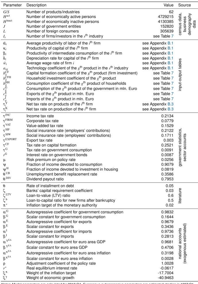
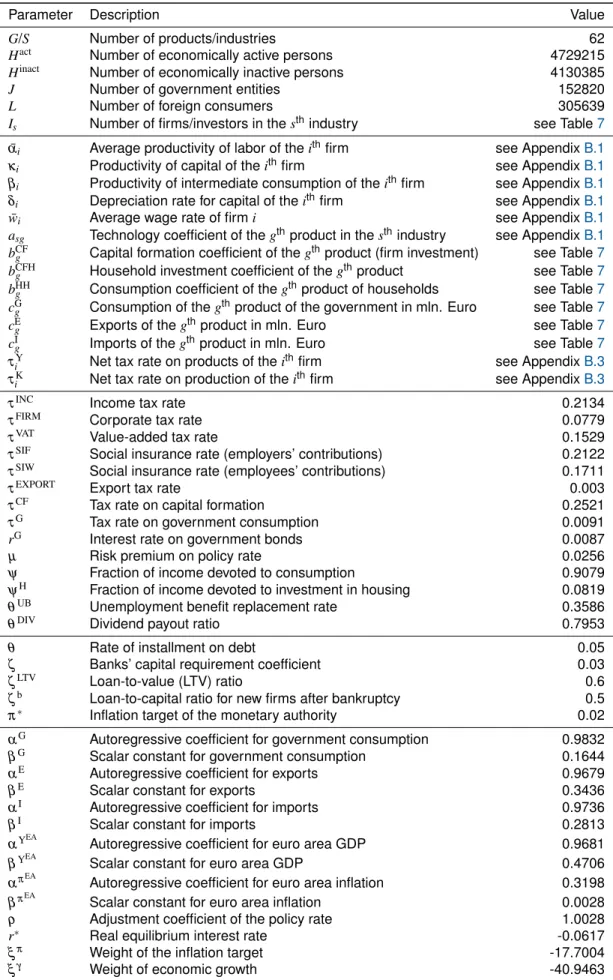
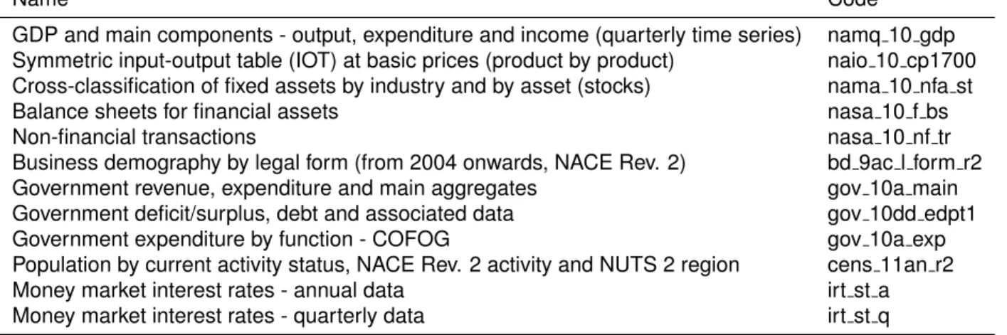
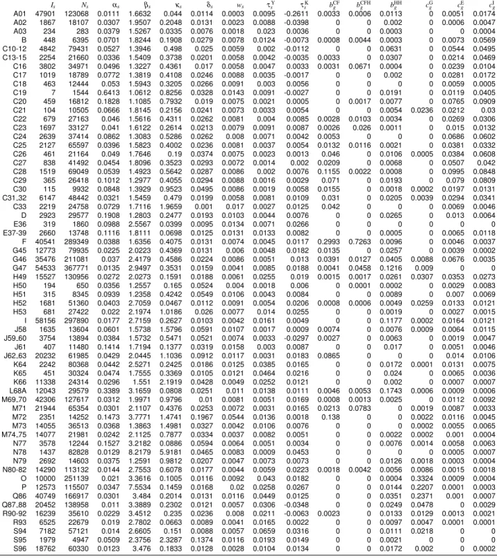
The parameters of our ABM are summarized in Table 1; for details see Appendix B. For the forecasting exercise in Section4, parameters were initially calculated and estimated over the sample 1997:Q1 to 2010:Q1 and then, respectively, re-estimated and recalculated, every quarter until 2013:Q4. Here we show, as an example, parameter values for 2010:Q4. Data sources include micro and macro data from national accounts, sector accounts, input-output tables, government statistics, census data, and business demography data; for details, see AppendixBand Table6. Model parameters are either taken directly from data or calculated from national accounting identities. Parameters that specify the number of agents are taken directly from census and business demography data. Model parameters concerning productivity and technology coefficients, as well as capital formation and consumption coefficients, are taken directly from input-output tables, or are derived from them. Tax rates and marginal propensities to consume or invest are calculated from national accounting identities.
Table 1. Model parameters
Parameter Description Value Source
G/S Number of products/industries 62 census data, business demog raph y data
Hact Number of economically active persons 4729215
Hinact Number of economically inactive persons 4130385
J Number of government entities 152820
L Number of foreign consumers 305639
Is Number of firms/investors in thesthindustry see Table7
¯
αi Average productivity of labor of theithfirm see AppendixB.1
input-output
tab
les
κi Productivity of capital of theithfirm see AppendixB.1
βi Productivity of intermediate consumption of theithfirm see AppendixB.1
δi Depreciation rate for capital of theithfirm see AppendixB.1
¯
wi Average wage rate of firmi see AppendixB.1
asg Technology coefficient of thegthproduct in thesthindustry see AppendixB.1
bCF
g Capital formation coefficient of thegthproduct (firm investment) see Table7
bCFH
g Household investment coefficient of thegthproduct see Table7
bHH
g Consumption coefficient of thegthproduct of households see Table7
cG
g Consumption of thegthproduct of the government in mln. Euro see Table7
cE
g Exports of thegthproduct in mln. Euro see Table7
cI
g Imports of thegthproduct in mln. Euro see Table7
τY
i Net tax rate on products of theithfirm see AppendixB.3
τK
i Net tax rate on production of theithfirm see AppendixB.3
τINC Income tax rate 0.2134
go ver nment statistics , sector accounts
τFIRM Corporate tax rate 0.0779
τVAT Value-added tax rate 0.1529
τSIF Social insurance rate (employers’ contributions) 0.2122
τSIW Social insurance rate (employees’ contributions) 0.1711
τEXPORT Export tax rate 0.003
τCF Tax rate on capital formation 0.2521
τG Tax rate on government consumption 0.0091
rG Interest rate on government bonds 0.0087
µ Risk premium on policy rate 0.0256
ψ Fraction of income devoted to consumption 0.9079
ψH Fraction of income devoted to investment in housing 0.0819
θUB Unemployment benefit replacement rate 0.3586
θDIV Dividend payout ratio 0.7953
θ Rate of installment on debt 0.05
liter
ature
ζ Banks’ capital requirement coefficient 0.03
ζLTV Loan-to-value (LTV) ratio 0.6
ζb Loan-to-capital ratio for new firms after bankruptcy 0.5
π∗ Inflation target of the monetary authority 0.02
αG Autoregressive coefficient for government consumption 0.9832
national
accounts
(e
xogenous
estimated)
βG Scalar constant for government consumption 0.1644
αE Autoregressive coefficient for exports 0.9679
βE Scalar constant for exports 0.3436
αI Autoregressive coefficient for imports 0.9736
βI Scalar constant for imports 0.2813
αYEA
Autoregressive coefficient for euro area GDP 0.9681
βYEA
Scalar constant for euro area GDP 0.4706
απEA
Autoregressive coefficient for euro area inflation 0.3198
βπEA
Scalar constant for euro area inflation 0.0028
ρ Adjustment coefficient of the policy rate 1.0028
r∗ Real equilibrium interest rate -0.0617
ξπ Weight of the inflation target -17.7004
ξγ Weight of economic growth -40.9463
These rates are set such that the financial flows observed in input-output tables, government statistics, and sector accounts are matched. Capital ratios and the inflation target of the monetary authority are set according to the literature. For exogenous processes such as imports and exports, parameters are estimated from national accounts (main aggregates).
4 Forecast performance
To validate the ABM, we conduct a series of forecasting exercises in which we evaluate the out-of-sample forecast performance of the ABM in comparison with standard macroeconomic modeling approaches.11
4.1 Comparison with VAR models
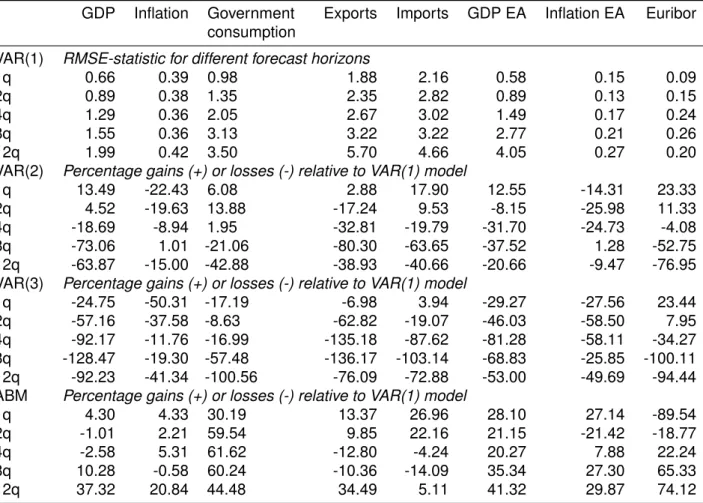
In this section, we compare the out-of-sample forecast performance of the ABM with that of various unconstrained (non-theoretical) VAR models estimated on the same observable macro time series in a traditional out-of-sample root mean squared error (RMSE)12forecast exercise. We compare the ABM with three standard VAR models of lag order one to three, estimated using the same eight observable time series. Observable time series include the real GDP, inflation, real government consumption, real exports and real imports of Austria, as well as real GDP and inflation of the euro area (EA), and the Euro Interbank Offered Rate (Euribor). To allow the data to decide on the degree of persistence and cointegration, in the VAR models we enter GDP, government consumption, exports, imports, and GDP of the EA in log levels. For this exercise, the VAR models and the ABM were initially estimated over the sample 1997:Q1 to 2010:Q1. The models were then used to forecast the eight time series from 2010:Q2 to 2016:Q4; the models were re-estimated every quarter. ABM results are obtained as an average over 500 Monte Carlo simulations.
Table2reports the out-of-sample RMSEs for different forecast horizons of 1, 2, 4, 8, and 12 quarters over the period 2010:Q2 to 2016:Q4. These out-of-sample forecast statistics demonstrate the good forecast performance of the ABM relative to the VAR models of different lag orders. For GDP and inflation, the ABM delivers a similar forecast performance to that of the VAR(1) for short- to medium-term horizons up to two years, and improves on it for longer horizons up to three years. For the other five variables (government consumption, exports, imports, GDP and inflation EA, Euribor), the ABM does better than the different VAR models by a considerable margin for almost all horizons. The forecast performances of the VAR(2) and especially the VAR(3) model clearly deteriorate for longer horizons.
4.2 Comparison with DSGE and AR models
In this section, we compare the out-of-sample forecast performance of the ABM to that of a standard DSGE model. As variables for this comparison, we choose the major macroeconomic aggregates: real GDP growth, inflation, and the main components of GDP—real household consumption and real investment. As a DSGE model, we employ a standard DSGE model ofSmets and Wouters(2007), which is a widely cited New Keynesian DSGE model for the US economy with sticky prices and wages, adapted to the Austrian economy. For this purpose, we use the two-country model ofBreuss and Rabitsch(2009), which is a New Open Economy Macro model for Austria as part of the European Monetary Union (EMU).13 The DSGE model is estimated on the following set of 13 variables for the same time period as the ABM (1997:Q1-2010:Q1): log difference of real GDP, real consumption, real investment and the real wage, log hours worked, the log difference of the GDP deflator (six each for Austria and the EA), as well as the three-month Euribor. As standard time series models for comparing the forecast performance of the ABM and DSGE models, we estimate AR models of lag orders one to three on the log levels of real GDP, real household consumption, real investment, and the log difference of the GDP deflator (inflation). Again, all models are initially estimated over the sample 1997:Q1 to 2010:Q1, and the models are then used to forecast the four time series from 2010:Q2 to 2016:Q4, with the models being re-estimated every quarter. ABM results are obtained as an average over 500 Monte Carlo simulations and the DSGE model is estimated using Bayesian methods.14
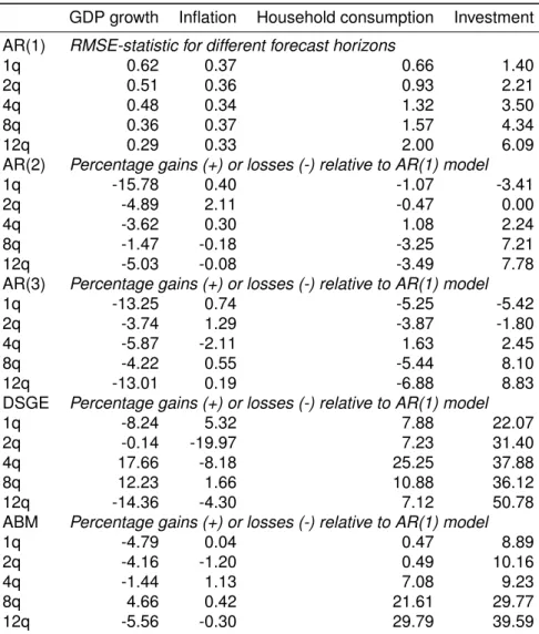
Table3 shows comparisons between the ABM and the DSGE and AR models of different lag orders for forecast horizons of 1, 2, 4, 8, and 12 quarters over the period 2010:Q2 to 2016:Q4. Similar to the forecast
11This out-of-sample prediction performance evaluation is constructed along the lines ofSmets and Wouters(2007), who compare a Bayesian DSGE model to unconstrained VAR as well as Bayesian VAR (BVAR) models.
12The root mean squared error is defined as follows:RMSE=q1
n∑Tt=1(ˆxt−xt)2, wherexˆtis the forecast value andxtis the observed data
point for time period t.
13See AppendixF.1for additional information on the DSGE model. We would like to thank Katrin Rabitsch for providing us with the improved version of the DSGE model inBreuss and Rabitsch(2009) for this manuscript.
14DSGE estimations are done with Dynare, seehttp://www.dynare.org/(Last accessed November 30th,2018). A sample of 250,000
Table 2.Out-of-sample forecast performance
GDP Inflation Government
consumption Exports Imports GDP EA Inflation EA Euribor VAR(1) RMSE-statistic for different forecast horizons
1q 0.66 0.39 0.98 1.88 2.16 0.58 0.15 0.09 2q 0.89 0.38 1.35 2.35 2.82 0.89 0.13 0.15 4q 1.29 0.36 2.05 2.67 3.02 1.49 0.17 0.24 8q 1.55 0.36 3.13 3.22 3.22 2.77 0.21 0.26 12q 1.99 0.42 3.50 5.70 4.66 4.05 0.27 0.20 VAR(2) Percentage gains (+) or losses (-) relative to VAR(1) model
1q 13.49 -22.43 6.08 2.88 17.90 12.55 -14.31 23.33 2q 4.52 -19.63 13.88 -17.24 9.53 -8.15 -25.98 11.33 4q -18.69 -8.94 1.95 -32.81 -19.79 -31.70 -24.73 -4.08 8q -73.06 1.01 -21.06 -80.30 -63.65 -37.52 1.28 -52.75 12q -63.87 -15.00 -42.88 -38.93 -40.66 -20.66 -9.47 -76.95 VAR(3) Percentage gains (+) or losses (-) relative to VAR(1) model
1q -24.75 -50.31 -17.19 -6.98 3.94 -29.27 -27.56 23.44 2q -57.16 -37.58 -8.63 -62.82 -19.07 -46.03 -58.50 7.95 4q -92.17 -11.76 -16.99 -135.18 -87.62 -81.28 -58.11 -34.27 8q -128.47 -19.30 -57.48 -136.17 -103.14 -68.83 -25.85 -100.11 12q -92.23 -41.34 -100.56 -76.09 -72.88 -53.00 -49.69 -94.44 ABM Percentage gains (+) or losses (-) relative to VAR(1) model
1q 4.30 4.33 30.19 13.37 26.96 28.10 27.14 -89.54 2q -1.01 2.21 59.54 9.85 22.16 21.15 -21.42 -18.77 4q -2.58 5.31 61.62 -12.80 -4.24 20.27 7.88 22.24 8q 10.28 -0.58 60.24 -10.36 -14.09 35.34 27.30 65.33 12q 37.32 20.84 44.48 34.49 5.11 41.32 29.87 74.12
Notes: All models are estimated starting in 1997:Q1. The forecast period is 2010:Q2 to 2016:Q4. All models are re-estimated each quarter. ABM results are obtained as an average over 500 Monte Carlo simulations.
exercise above, the AR(1) overall turns out to perform better than the AR models of lag orders two and three. Regarding forecasts of GDP growth and inflation, the performance of the ABM, DSGE, and AR(1) model is relatively similar, with the DSGE model applying more filtering than the other models. Both the ABM and the DSGE models show their strengths in terms of forecasts of household consumption, and especially investment, as theory-driven economic models. Both these models explicitly incorporate the behavior of different agents in the economy, as well as constraints due to the consistency requirements of national accounting—for example, they take into consideration that household consumption and investment are major components of GDP. While the improvement for household consumption is clearly noticeable—especially for the DSGE model, whose sophisticated assumptions about agents’ behavior seem to make the greatest difference for this variable—there is also quite a pronounced improvement for investment. For investment forecasts, both the ABM and the DSGE model clearly do better than the AR(1) model, especially for longer horizons.
4.3 Conditional forecasts
As a further validation exercise, we test the conditional forecast performance of the different model classes (ABM, DSGE, and AR models). In this exercise, we generate forecasts from the three models conditional on the paths realized for the following three variables: real exports, real imports, and real government consumption (as government consumption is an exogenous shock in the DSGE model, conditional forecasts in the DSGE models are subject to exogenous paths for exports and imports). The exogenous predictors can be included in the AR model and the ABM in a straightforward way; for details, see AppendixD. Conditional forecasts in the DSGE model are achieved by controlling certain shocks to match the predetermined paths of the exogenous predictors. In particular, we control the consumption preference shocks for Austria and the EA, which are the major drivers for Austrian exports and imports in the two-country setting of the DSGE model; see AppendixF.12for details. Again, we use the period 1997:Q1-2010:Q1 to initially estimate our models. We then forecast real GDP growth, inflation, and nominal household consumption and investment from 2010:Q2 to 2016:Q4, with the models being
Table 3.Out-of-sample forecast performance in comparison to DSGE model GDP growth Inflation Household consumption Investment AR(1) RMSE-statistic for different forecast horizons
1q 0.62 0.37 0.66 1.40
2q 0.51 0.36 0.93 2.21
4q 0.48 0.34 1.32 3.50
8q 0.36 0.37 1.57 4.34
12q 0.29 0.33 2.00 6.09
AR(2) Percentage gains (+) or losses (-) relative to AR(1) model
1q -15.78 0.40 -1.07 -3.41
2q -4.89 2.11 -0.47 0.00
4q -3.62 0.30 1.08 2.24
8q -1.47 -0.18 -3.25 7.21
12q -5.03 -0.08 -3.49 7.78
AR(3) Percentage gains (+) or losses (-) relative to AR(1) model
1q -13.25 0.74 -5.25 -5.42
2q -3.74 1.29 -3.87 -1.80
4q -5.87 -2.11 1.63 2.45
8q -4.22 0.55 -5.44 8.10
12q -13.01 0.19 -6.88 8.83
DSGE Percentage gains (+) or losses (-) relative to AR(1) model
1q -8.24 5.32 7.88 22.07
2q -0.14 -19.97 7.23 31.40
4q 17.66 -8.18 25.25 37.88
8q 12.23 1.66 10.88 36.12
12q -14.36 -4.30 7.12 50.78
ABM Percentage gains (+) or losses (-) relative to AR(1) model
1q -4.79 0.04 0.47 8.89
2q -4.16 -1.20 0.49 10.16
4q -1.44 1.13 7.08 9.23
8q 4.66 0.42 21.61 29.77
12q -5.56 -0.30 29.79 39.59
Notes: All models are estimated starting in 1997:Q1. The forecast period is 2010:Q2 to 2016:Q4. All models are re-estimated each quarter. ABM results are obtained as an average over 500 Monte Carlo simulations.
re-estimated every quarter. Thus, together with the real exports, real imports, and real government consumption, we account for all main components of GDP.
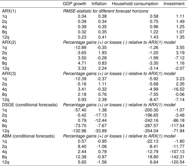
Table4shows that the forecast performance of the ABM and AR models improves pronouncedly for GDP growth and household consumption and investment when exogenous predictors are included. Similar to the forecast exercise above, the ARX(1) turns out overall to perform better than the ARX models of lag orders two and three. Again, the performance of the ABM (conditional forecasts) and ARX(1) model is relatively similar for GDP growth and inflation. However, compared to the unconditional case, the ABM as a theory-driven model does not better in forecasting household consumption and investment. The forecast performance of the DSGE model (conditional forecasts) clearly deteriorates for all variables for longer horizons. This is for methodological reasons, that is, the need to control exogenous shocks such that the exogenous paths of the predictors are matched in the DSGE model. This clearly has the most pronounced implications for the forecast of household consumption in the DSGE model, where forecast errors increase to a large extent when compared to the ARX(1) model.
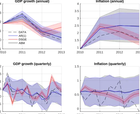
Figures1,2and3provide a graphical comparison between conditional forecasts with the ABM and results from an ARX(1) model, and between conditional forecasts with the DSGE model and actual time series data reported by Eurostat. Figure1shows aggregate GDP growth and inflation (measured by GDP deflator) rates— annually (top) and quarterly (bottom). One can see at first glance that the ABM tracks the data very well for GDP growth (left panels). For annualized (top left) and quarterly (bottom left) model results, almost all data points are within the 90 percent confidence interval (gray shaded area)—except for two outliers (2011:Q1,2012:Q2), where the Austrian growth rate either picked up quite sharply (2011:Q1) or decreased considerably, despite an upward trend before (2012:Q2). It is especially interesting to note how the ABM catches trends in the data somewhat better than the ARX(1) model. In particular, the ABM reacts directly to a fall in exports in 2013:Q1 (see Figure
Table 4.Conditional forecast performance
GDP growth Inflation Household consumption Investment
ARX(1) RMSE-statistic for different forecast horizons
1q 0.34 0.38 0.58 1.11
2q 0.39 0.34 0.75 1.49
4q 0.38 0.35 0.96 1.25
8q 0.32 0.35 1.22 1.07
12q 0.23 0.41 1.43 1.35
ARX(2) Percentage gains (+) or losses (-) relative to ARX(1) model
1q -12.89 -0.35 -1.26 3.55
2q -3.65 1.93 -1.20 3.19
4q 3.50 -0.28 -1.99 -7.12
8q 4.71 0.83 -3.30 1.16
12q 3.33 2.24 -3.14 -2.07
ARX(3) Percentage gains (+) or losses (-) relative to ARX(1) model
1q -12.39 -2.37 -5.92 3.23
2q -5.16 1.11 -5.68 2.35
4q 3.41 -0.32 -4.99 -16.52
8q 2.18 0.76 -7.55 -0.06
12q 0.93 2.39 -8.47 -7.14
DSGE (conditional forecasts) Percentage gains (+) or losses (-) relative to ARX(1) model
1q -57.40 1.38 -200.30 -1.07
2q -5.42 -17.13 -196.65 -3.48
4q 0.79 -12.44 -242.16 -86.18
8q -73.70 -7.67 -287.57 -117.54
12q -132.96 -33.89 -354.04 -71.94
ABM (conditional forecasts) Percentage gains (+) or losses (-) relative to ARX(1) model
1q 0.57 -0.95 -22.13 -1.80
2q 8.40 -1.06 -8.41 -11.77
4q 2.44 0.78 -12.79 -107.13
8q 12.38 -0.97 18.80 -142.31
12q 5.65 -1.56 6.64 -120.54
Notes: All models are estimated starting in 1997:Q1. The forecast period is 2010:Q2 to 2016:Q4. All models are re-estimated each quarter. ABM results are obtained as an average over 500 Monte Carlo simulations.
3)—which reflects a slowdown in economic growth for some of Austria’s European trading partners during the European debt crisis—that drags down GDP growth in the ABM. In contrast to this, the ARX(1) model simply extrapolates the past trend into the future. Similar to the ABM, the DSGE in a conditional forecasting setup seems to catch upward and downward trends in the data quite well, but tends to “overreact” by taking the trend too far. This certainly deteriorates the forecast performance of the DSGE, and is most probably connected to the way in which controlling the shocks for the conditional forecasting procedure influences the mechanics of the DSGE model.
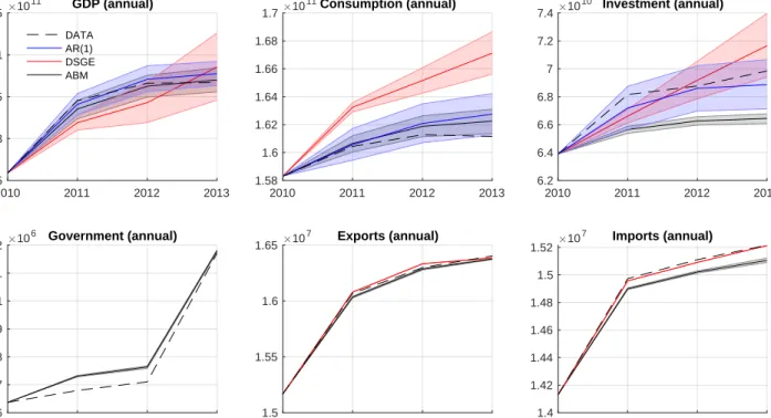
A similar picture arises when the conditional forecasts for the main macroeconomic aggregates in levels (GDP, household consumption, investment) of the ABM are compared to the other models; see Figures2(annual) and 3(quarterly). Looking at GDP at annual levels (top left in Figure2) and quarterly levels (top left in Figure3), it is evident that the ABM closely follows the data, as do the growth rates in Figure1, and that all data points, except for the two outliers referred to above, are within the confidence interval. The ARX(1) model delivers a comparable forecasting performance, but smooths the trends more than the ABM does. The DSGE model at first consistently underestimates both annual and quarterly GDP levels, and then overestimates the upward trend starting in 2013:Q2. Again, the influence on quarterly GDP of the drop in exports in 2013:Q1, due to overall economic developments in Europe during the European debt crisis (Figure3, bottom middle panel), remains visible, and the ABM captures this trend quite well. Both the ABM and the ARX(1) model seem to smooth out the changes in household consumption to approximately match the average trend, with the ABM being somewhat closer to the data. Again, the DSGE model seems to follow the trends in the data quite accurately, but consistently overestimates the level, which might be responsible for the overall poor forecasting performance of the DSGE model for household consumption. As to be expected, the volatility of investment in the data is the highest of all
2010 2011 2012 2013 -1 0 1 2 3 4 GDP growth (annual) DATA AR(1) DSGE ABM 2010 2011 2012 2013 1 1.5 2 2.5 3 3.5 4 Inflation (annual) 2010 2011 2012 2013 -1 -0.5 0 0.5 1 1.5 2 GDP growth (quarterly) 2010 2011 2012 2013 0 0.5 1 1.5 Inflation (quarterly)
Figure 1.Forecast performance from 2011:Q1-2013:Q4. ABM conditional forecasts (black line), DSGE
conditional forecasts (red line), ARX(1) forecasts (blue line) and observed Eurostat data for Austria (dashed line). Top figures show growth and inflation on an annualized basis; bottom figures depict quarterly growth and inflation rates. A 90 percent confidence interval is plotted around the mean trajectory. Model results are obtained as an average over 500 Monte Carlo simulations.
these variables. The ARX(1) smoothes this volatility out on average, and is thus very successful in tracking both annual and quarterly investment data (Figures2and3, top right). The DSGE model, while catching the initial trend in the data, overshoots in its forecast at the end, whereas the ABM consistently underestimates investment levels.
4.4 Components of GDP
The previous section has demonstrated that the size and detailed structure of the ABM tend to improve its forecasting performance compared to standard models. Another important advantage of our approach is the possibility of breaking down simulation results in a stock-flow consistent way according to national accounting (ESA). In particular, we are able to report results for all economic activities depicted in this model consistent with national accounting rules, in addition to relating them to the main macroeconomic aggregates. Most importantly, for all simulations and forecasts, our model preserves the principle of double-entry bookkeeping. This implies that all financial flows within the model are made explicit and are recorded as an outflow of money (use of funds) for one agent in the model in relation to a certain economic activity, and as an inflow of money (source of funds) for another agent. In principle, we can thus consistently report on the economic activity of every single agent at the micro-level. A more informative aggregation is on a meso-level according to the NACE/CPA classification into 64 industries, which encompasses many variables. This multitude of results consists of all components of GDP on a sectoral level: among others, wages, operating surplus, investment, taxes and subsidies of different kinds, intermediate inputs, exports, imports, final consumption of different agents (household, government), employment, and also economic indicators such as productivity coefficients for capital, labor, and intermediate inputs. Probably the simplest example indicative of this model structure is that it breaks down simulation results into the larger components of GDP.
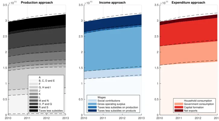
Figure4is a graphical representation of the conditional ABM forecasts from Section4.3decomposed for these larger components of GDP. The components are shown according to the production, income, and expenditure approaches to determining GDP, which are defined within the framework of our model along ESA lines, as laid out in equation (E.1). With the fine-grained detail incorporated into our model, we can demonstrate how the development of macroeconomic aggregates such as GDP relates to trends in different industry sectors (production approach), the distribution of national income (income approach), and the composition of final uses in the economy (expenditure approach). Here, the colored fields indicate ABM simulation results for the different
2010 2011 2012 2013 2.95 3 3.05 3.1 3.15 10 11 GDP (annual) DATA AR(1) DSGE ABM 2010 2011 2012 2013 1.58 1.6 1.62 1.64 1.66 1.68 1.7 10 11Consumption (annual) 2010 2011 2012 2013 6.2 6.4 6.6 6.8 7 7.2 7.4 10 10 Investment (annual) 2010 2011 2012 2013 6.06 6.07 6.08 6.09 6.1 6.11 6.12 10 6 Government (annual) 2010 2011 2012 2013 1.5 1.55 1.6 1.65 10 7 Exports (annual) 2010 2011 2012 2013 1.4 1.42 1.44 1.46 1.48 1.5 1.52 10 7 Imports (annual)
Figure 2.Forecast performance from 2011:Q1-2013:Q4. GDP (annually, in euro and in real terms with base year 2010), household consumption (annually, in euro and in real terms with base year 2010), fixed investment (annually, in euro and in real terms with base year 2010), government consumption (annually, in euro and in real terms with base year 2010), exports (annually, in euro and in real terms with base year 2010), and imports (annually, in euro and in real terms with base year 2010). ABM conditional forecasts (black line), DSGE
conditional forecasts (red line), ARX(1) forecasts (blue line), and observed Eurostat data for Austria (dashed line). A 90 percent confidence interval is plotted around the mean trajectory. Model results are obtained as an average over 500 Monte Carlo simulations.
components of GDP, while the dashed line refers to the values reported in the data. Our results show that ABM forecasts of these components of GDP, where the ABM does not predict major structural changes for the Austrian economy, correspond closely to the developments in the data.
4.5 Sectoral decomposition
The detailed structure of the ABM allows macroeconomic forecasts to be broken down into varying levels of detail, offering insights into the composition of overall macroeconomic trends. Figure5shows ABM forecasts for gross value added (GVA) generated within the industry sectors in comparison with the data for the conditional forecasting setup (see Table8for a detailed list of industry sectors).15 The projections of the ABM capture the trends in larger sectors particularly well. Most notably, trends in major sectors such as construction and construction works (F), retail trade (G47), accommodation and food services (I), or land transport services (H49) are matched by the ABM in close relation to the data. These sectors tend to follow overall trends in GDP to a large degree, which is one explanation for the good forecasting performance of the ABM for these sectors.
Some of the more pronounced differences are due to sector-specific features such as sizeable export-induced exogenous shocks or an unusually low number of firms in the sector, which can cause sectors to deviate from aggregate macroeconomic trends. This is especially true for smaller sectors, where deviations of ABM forecasts are higher in relative terms. This is especially relevant to products of agriculture, hunting and related services (A01), mining and quarrying (B), air transport services (H51), motion picture, video, and television program services (J59), and telecommunication services (J61), among others. For manufacturing sectors, which are potentially influenced more by trends exogenous to the ABM, such as the structure of Austrian exports, the forecasts are within an acceptable range, which is often also the case for larger sectors. Indicative examples for such sectors are wood and products of wood (C16), fabricated metal products (C25), and machinery and equipment (C28).
2010 2011 2012 2013 7.4 7.5 7.6 7.7 7.8 7.9 8 10 10 GDP (quarterly) DATA AR(1) DSGE ABM 2010 2011 2012 2013 3.9 4 4.1 4.2 4.3 10 10Consumption (quarterly) 2010 2011 2012 2013 1.6 1.65 1.7 1.75 1.8 1.85 1.9 10 10Investment (quarterly) 2010 2011 2012 2013 1.51 1.515 1.52 1.525 1.53 1.535 1.54 10 6Government (quarterly) 2010 2011 2012 2013 3.85 3.9 3.95 4 4.05 4.1 4.15 10 6 Exports (quarterly) 2010 2011 2012 2013 3.6 3.65 3.7 3.75 3.8 3.85 3.9 10 6 Imports (quarterly)
Figure 3.Forecast performance from 2011:Q1-2013:Q4. GDP (quarterly, in euro and in real terms with base year 2010), household consumption (quarterly, in euro and in real terms with base year 2010), fixed investment (quarterly, in euro and in real terms with base year 2010), government consumption (quarterly, in euro and in real terms with base year 2010), exports (quarterly, in euro and in real terms with base year 2010), and imports (quarterly, in euro and in real terms with base year 2010). ABM conditional forecasts (black line), DSGE
conditional forecasts (red line), ARX(1) forecasts (blue line), and observed Eurostat data for Austria (dashed line). A 90 percent confidence interval is plotted around the mean trajectory. Model results are obtained as an average over 500 Monte Carlo simulations.
Production approach 2010 2011 2012 2013 0 0.5 1 1.5 2 2.5 3 3.5 10 11 A B, C, D and E F G, H and I J K L M and N O, P and Q R and S Taxes less subsidies
Income approach 2010 2011 2012 2013 0 0.5 1 1.5 2 2.5 3 3.5 10 11 Wages Social contributions Gross operating surplus Taxes less subsidies on production Taxes less subsidies on products
Expenditure approach 2010 2011 2012 2013 0 0.5 1 1.5 2 2.5 3 3.5 10 11 Household consumption Government consumption Capital formation Net exports
Figure 4.Composition of GDP according to production, income and expenditure approaches. The colored areas indicate ABM simulation results for one selected time period (2011:Q1-2013:Q4), again as an average over 500 Monte Carlo simulations. The dashed line shows the corresponding values obtained from the data.
2010 2011 2012 2013 2000 2200 2400 2600 A01 2010 2011 2012 2013 1050 1100 1150 1200 A02 2010 2011 2012 2013 14 16 18 20 22 A03 2010 2011 2012 2013 800 1000 1200 B 2010 2011 2012 2013 4600 4800 5000 C10-C12 2010 2011 2012 2013 900 1000 1100 C13-C15 2010 2011 2012 2013 1600 1700 1800 C16 2010 2011 2012 2013 1600 1650 1700 C17 2010 2011 2012 2013 800 900 1000 C18 2010 2011 2012 2013 0 100 200 C19 2010 2011 2012 2013 1000 1200 1400 C20 2010 2011 2012 2013 1200 1250 1300 1350 C21 2010 2011 2012 2013 1700 1800 1900 C22 2010 2011 2012 2013 1900 2000 2100 2200 C23 2010 2011 2012 2013 2900 3000 3100 3200 C24 2010 2011 2012 2013 3800 4000 4200 4400 C25 2010 2011 2012 2013 1800 2000 2200 C26 2010 2011 2012 2013 3000 3200 3400 3600 C27 2010 2011 2012 2013 4500 5000 5500 6000 C28 2010 2011 2012 2013 2400 2600 2800 3000 C29 2010 2011 2012 2013 800 900 1000 C30 2010 2011 2012 2013 2100 2200 2300 C31_C32 2010 2011 2012 2013 3000 3200 3400 C33 2010 2011 2012 2013 4400 4600 4800 5000 5200 D 2010 2011 2012 2013 400 500 600 E36 2010 2011 2012 2013 2600 2700 2800 2900 E37-E39 2010 2011 2012 2013 1.7 1.75 1.8 1.85 10 4 F 2010 2011 2012 2013 3600 3800 4000 G45 2010 2011 2012 2013 1.8 1.9 2 10 4 G46 2010 2011 2012 2013 1.25 1.3 1.35 1.4 10 4 G47 2010 2011 2012 2013 6500 7000 7500 8000 H49 2010 2011 2012 2013 18 20 22 24 H50 2010 2011 2012 2013 400 500 600 H51 2010 2011 2012 2013 5000 5200 5400 5600 H52 2010 2011 2012 2013 1250 1300 1350 1400 H53 2010 2011 2012 2013 1.3 1.4 1.5 10 4 I 2010 2011 2012 2013 1150 1200 1250 1300 J58 2010 2011 2012 2013 800 900 1000 J59_J60 2010 2011 2012 2013 2400 2600 2800 3000 J61 2010 2011 2012 2013 5000 6000 7000 J62_J63 2010 2011 2012 2013 7500 8000 8500 9000 K64 2010 2011 2012 2013 2200 2400 2600 K65 2010 2011 2012 2013 900 1000 1100 1200 K66 2010 2011 2012 2013 2.6 2.8 3 10 4 L 2010 2011 2012 2013 7500 8000 8500 M69_M70 2010 2011 2012 2013 4000 4500 5000 M71 2010 2011 2012 2013 6000 7000 8000 M72 2010 2011 2012 2013 1400 1600 1800 M73 2010 2011 2012 2013 1000 1100 1200 M74_M75 2010 2011 2012 2013 5000 5200 5400 5600 N77 2010 2011 2012 2013 3800 4000 4200 N78 2010 2011 2012 2013 400 450 500 550 N79 2010 2011 2012 2013 4000 4200 4400 4600 N80-N82 2010 2011 2012 2013 1.35 1.4 1.45 1.5 10 4 O 2010 2011 2012 2013 1.3 1.35 1.4 1.45 10 4 P 2010 2011 2012 2013 1.3 1.35 1.4 1.45 10 4 Q86 2010 2011 2012 2013 4000 4200 4400 4600 Q87_Q88 2010 2011 2012 2013 2200 2300 2400 R90-R92 2010 2011 2012 2013 1050 1100 1150 1200 R93 2010 2011 2012 2013 1700 1800 1900 2000 S94 2010 2011 2012 2013 550 600 650 S95 2010 2011 2012 2013 2000 2100 2200 S96 Figure 5. Compar ison of sector al gross value added (GV A) for model sim ulations and obser ved data of A ustr ia. GV A gener ated by on e representativ e time per iod (500 Monte Car lo sim ulations) is sho wn by a solid line (a 90 percent confidence inter val is plotted aroun d the mean trajector y), and obser ved GV A in A ustr ia from 2010 to 2013 is indicated by a dashed line .GV A is disagg regated for 64 economic activities/products (NA CE*64, CP A*64) according to the statistical classification of economic activities in the European Comm unity (NA CE Re v. 2).
5 Conclusion
We have developed an ABM of a small open economy that fits micro and macro data from national accounts, sector accounts, input-output tables, government statistics, census data, and business demography data. Although the model is very detailed, it is able to compete with standard VAR, AR, and DSGE models in out-of-sample forecasting. An advantage of our detailed ABM is that it allows for a breakdown of the forecasts of aggregate variables in a stock-flow consistent manner to generate forecasts of disaggregated sectoral variables and the main components of GDP.
The ABM is tailor-made for the small open economy of Austria, but the model can easily be adapted to other economies of larger countries such as the UK and the US or to larger regions such as the EU. Such extensions and applications are currently being explored. Our detailed ABM can also be used for stress-testing exercises or for predicting the effect of changes in monetary, fiscal, and other macroeconomic policies.
Our model is the first ABM that can compete in out-of-sample forecasting of macro variables. A grand challenge for future work would be a “big data ABM” research program to develop ABMs for larger economies and regions based on available micro and macro data to eventually monitor the macro economy in real time on supercomputers. Such detailed “big data ABMs” have the potential for improved macro forecasting and more reliable policy scenario analysis.
References
An, S. and Schorfheide, F. (2007). Baysian analysis of dsge models. Econometric Reviews, Vol. 26, Iss. 2-4:113–172.
Arthur, W. B., Holland, J. H., LeBaron, B., Palmer, R., and Tayler, P. (1997). Asset pricing under endogenous expectations in an artificial stock market. In Arthur, W. B., Durlauf, S., and Lane, D., editors,The Economy as an Evolving Complex System II. Addison-Wesley, Reading, MA, U.S.A.
Ashraf, Q., Gershman, B., and Howitt, P. (2017). Banks, market organization, and macroeconomic performance: an agent-based computational analysis.Journal of Economic Behavior & Organization, 135:143–180. Assenza, T., Delli Gatti, D., and Grazzini, J. (2015). Emergent dynamics of a macroeconomic agent based model
with capital and credit. Journal of Economic Dynamics and Control, 50:5–28. Axtell, R. L. (2001). Zipf distribution of us firm sizes.Science, 293(5536):1818–1820.
Axtell, R. L. (2018). Endogenous firm dynamics and labor flows via heterogeneous agents. In Hommes, C. and LeBaron, B., editors,Handbook of Computational Economics, volume 4 ofHandbook of Computational Economics, pages 157 – 213. Elsevier.
Baptista, R., Farmer, J. D., Hinterschweiger, M., Low, K., Tang, D., and Uluc, A. (2016). Macroprudential policy in an agent-based model of the uk housing market. Staff Working Paper 619, Bank of England.
Blanchard, O. (2016). Do dsge models have a future? PIIE Policy Brief, PB 16-11.
Blattner, T. S. and Margaritov, E. (2010). Towards a robust monetary policy rule for the euro area. ECB Working Paper No. 1210.
Brayton, F., Mauskopf, E., Reifschneider, D., Tinsley, P., Williams, J., Doyle, B., and Sumner, S. (1997). The role of expectations in the frb/us macroeconomic model.Federal Reserve Bulletin, April 1997.
Breuss, F. and Rabitsch, K. (2009). An estimated two-country dsge model auf austria and the euro area.Empirica, 36:123–158.
Brunnermeier, M. K., Eisenbach, T. M., and Sannikov, Y. (2013). Macroeconomics with financial frictions: A survey. InAdvances in Economics and Econometrics, Tenth World Congress of the Econometric Society. New York: Cambridge University Press.
Calvo, G. A. (1983). Staggered prices in a utility-maximizing framework. Journal of monetary Economics, 12(3):383–398.
Canova, F. and Sala, L. (2009). Back to square one: Identification issues in dsge models.Journal of Monetary Economics, 56:431 – 449.
Christiano, L. J., Eichenbaum, M. S., and Trabandt, M. (2018). On DSGE models. Journal of Economic Perspectives, 32(3):113–40.
Christiano, L. J., Trabandt, M., and Walentin, K. (2010). Dsge models for monetary policy analysis. NBER Working Paper 16074.
Cincotti, S., Raberto, M., and Teglio, A. (2010). Credit money and macroeconomic instability in the agent-based model and simulator eurace.Economics: The Open-Access, Open-Assessment E-Journal, 4.
Colander, D., Goldberg, M., Haas, A., Juselius, K., Kirman, A., Lux, T., and Sloth, B. (2009). The financial crisis and the systemic failure of the economics profession. Critical Review, 21:2-3:249 – 267.
Colander, D., Howitt, P., Kirman, A., Leijonhufvud, A., and Mehrling, P. G. (2008). Beyond dsge models: Toward an empirically based macroeconomics. American Economic Review, Papers and Proceedings, Vol. 98 No. 2:236–240.
Dawid, H. and Delli Gatti, D. (2018). Agent-based macroeconomics. In Hommes, C. and LeBaron, B., editors,
Handbook of Computational Economics, volume 4 ofHandbook of Computational Economics, pages 63 – 156. Elsevier.
Dawid, H., Harting, P., van der Hoog, S., and Neugart, M. (2018). Macroeconomics with heterogeneous agent models: fostering transparency, reproducibility and replication. Journal of Evolutionary Economics.
Delli Gatti, D., Desiderio, S., Gaffeo, E., Cirillo, P., and Gallegati, M. (2011).Macroeconomics from the Bottom-up. Springer Milan.
Dosi, G., Napoletano, M., Roventini, A., and Treibich, T. (2017). Micro and macro policies in the keynes+schumpeter evolutionary models.Journal of Evolutionary Economics, 27:63 – 90.
Eurostat (2013).European System of Accounts: ESA 2010. EDC collection. Publications Office of the European Union.
Evans, G. W. and Honkapohja, S. (2001).Learning and expectations in macroeconomics. Princeton University Press.
Fagiolo, G. and Roventini, A. (2017). Macroeconomic policy in dsge and agent-based models redux: New developments and challenges ahead.Journal of Artificial Societies and Social Simulation, 20(1).
Farmer, J. D. and Foley, D. (2009). The economy needs agent-based modelling. Nature, 460:685 – 686. Fernandez-Villaverde, J. (2010). The econometrics of dsge models. J. SERIEs, Volume 1, Issue 1:3–49. Freeman, R. B. (1998). War of the models: Which labour market institutions for the 21st century? Labour
Economics, 5:1–24.
Geanakoplos, J., Axtell, R. L., Farmer, J. D., Howitt, P., Conlee, B., Goldstein, J., Hendrey, M., Palmer, N. M., and Yang, C.-Y. (2012). Measuring system risk: Getting at systemic risk via an agent-based model of the housing market.American Economic Review: Papers and Proceedings, 102(3):53–58.
Gintis, H. (2007). The dynamics of general equilibrium.The Economic Journal, 117 (October):1280 – 1309. Haldane, A. G. and Turrell, A. E. (2018). An interdisciplinary model for macroeconomics. Oxford Review of
Economic Policy, 34(1-2):219–251.
Hommes, C. (2018). Behavioral & experimental macroeconomics and policy analysis: a complex systems approach. Journal of Economic Literature. forthcoming.
Hommes, C., Mavromatis, K., ¨Ozden, T., and Zhu, M. (2019). Behavioral learning equilibria in the new keynesian model.Working Paper Dutch Central Bank.
Hommes, C. and Zhu, M. (2014). Behavioral learning equilibria.Journal of Economic Theory, 150:778–814. Ijiri, Y. and Simon, H. A. (1977). Skew distributions and the sizes of business firms. North-Holland.
Kirman, A. (2010). The economic crisis is a crisis for economic theory.CESifo Economic Studies, 56 (4):498–535. Klimek, P., Poledna, S., Farmer, J. D., and Thurner, S. (2015). To bail-out or to bail-in? answers from an
agent-based model.Journal of Economic Dynamics and Control, 50:144–154.
Krugman, P. (2011). The profession and the crisis.Eastern Economic Journal, 37:307 – 312.
LeBaron, B. and Tesfatsion, L. (2008). Modeling macroeconomies as open-ended dynamic systems of interacting agents.AER Papers and Proceedings, Vol. 98, No. 2:246 –250.
Leeper, E. M. and Zha, T. (2003). Modest policy interventions.Journal of Monetary Economics, 50(8):1673–1700. Linde, J., Smets, F., and Wouters, R. (2016). Challenges for central banks’ macro models. Sveriges Riksbank
Working Paper Series, 323.
Lux, T. and Zwinkels, R. C. J. (2018). Empirical validation of agent-based models. In Hommes, C. and LeBaron, B., editors,Handbook of Computational Economics, volume 4 ofHandbook of Computational Economics, pages 437 – 488. Elsevier.