An Efficient Euler Method to Predict Shock Migration on a Straked Delta Wing Design

(1)

Air Force Institute of Technology

AFIT Scholar

Theses and Dissertations Student Graduate Works

3-22-2018

An Efficient Euler Method to Predict Shock

Migration on a Straked Delta Wing Design

Dylan N. Hope

Follow this and additional works at:https://scholar.afit.edu/etd Part of theAerodynamics and Fluid Mechanics Commons

This Thesis is brought to you for free and open access by the Student Graduate Works at AFIT Scholar. It has been accepted for inclusion in Theses and Dissertations by an authorized administrator of AFIT Scholar. For more information, please [email protected].

Recommended Citation

Hope, Dylan N., "An Efficient Euler Method to Predict Shock Migration on a Straked Delta Wing Design" (2018).Theses and Dissertations. 1772.

(2)

An Efficient Euler Method to Predict Shock Migration on an Oscillating

Straked Delta Wing Design

THESIS

Dylan N. Hope, 2nd Lt, USAF

AFIT-ENY-MS-18-M-264

DEPARTMENT OF THE AIR FORCE AIR UNIVERSITY

AIR FORCE INSTITUTE OF TECHNOLOGY

Wright-Patterson Air Force Base, Ohio

DISTRIBUTION STATEMENT A. APPROVED FOR PUBLIC RELEASE; DISTRIBUTION UNLIMITED.

(3)

The views expressed in this thesis are those of the author and do not reflect the official policy or position of the United States Air Force, Department of Defense, or the United States Government.

(4)

An Efficient Euler Method to Predict

Shock Migration on an Oscillating

Straked Delta Wing Design

THESIS

Presented to the Faculty

Department of Aeronautics and Astronautics Graduate School of Engineering and Management

Air Force Institute of Technology Air University

Air Education and Training Command In Partial Fulfillment of the Requirements for the Degree of Master of Science in Aeronautical Engineering

Dylan N. Hope, BSAE 2nd Lt, USAF

March, 2018

DISTRIBUTION STATEMENT A. APPROVED FOR PUBLIC RELEASE; DISTRIBUTION UNLIMITED.

(5)

Abstract

In support of the Air Force Office of Scientific Research, this project sought to identify the significance of nonlinear aerodynamic phenomena in regards to LCO of a straked delta wing design. Previous works include unsteady Navier-Stokes aeroelastic analysis of various wing designs and flight test of F-16 transonic LCO with interest focused on oscillatory SITES behavior. The research presented within this investi-gation further expanded the understanding of unsteady aerodynamics by performing aeroelastic analysis of a wing oscillated in pitch with an Euler-based, boundary layer coupled numerical method (ZEUS).

The wing was tested for a multitude of LCO parameters such as median AoA, oscillation amplitude, oscillation frequency, Mach number, and the type of numerical solver used. Computed pressure data sets were analyzed along the wing’s surface at 4 chordwise stations along the wing’s span.

Results indicate that oscillatory shock migration occurs in response to the pitch-ing motion of the wpitch-ing. ZEUS has the capability to run either a fully inviscid solution or a boundary layer coupled solution (BLC). While the use of both methods found shock migration to occur, the BLC solution predicted more significant shock migra-tion. The inviscid solution predicted more aggressive shocks located further aft on the wing than the BLC solution. In regards to oscillation amplitude, increasing the amplitude resulted in a greater range of shock migration than lower amplitude cases. Both oscillation frequencies tested did not show any noteworthy differences. The aforementioned findings support the theory that potential oscillatory shock migration can occur during certain cases of transonic LCO. In addition, it was concluded that based on the flow solver used (ZEUS), shock movement during LCO is not purely a function of viscosity (SITES), although the modeling of viscous effects does affect the range of shock migration.

(6)

List of Figures

Figure Page

1.1 Example of LCO. . . 3 2.1 Flow features on an airfoil at and above the critical Mach number.

(Federal Aviation Administration, 2004: 15-7) . . . 13 2.2 Simple Wing/Strake Configuration. Pressure sensors are located

along the dotted lines labled 1-4. (dimensions in mm) [8] . . . 21 2.3 Dimensions of wing panel (dimensions in mm) [8]. The

computa-tional model used in this study is slightly different than the model presented here. . . 22 2.4 An example of a test matrix used in Cunninghman’s experiment. [8] 23 3.1 Mesh Generation, Top View, Close. XY plane view of the

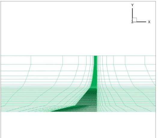
compu-tational mesh. . . 26 3.2 Mesh Generation, Top View, Full. XY plane view of the

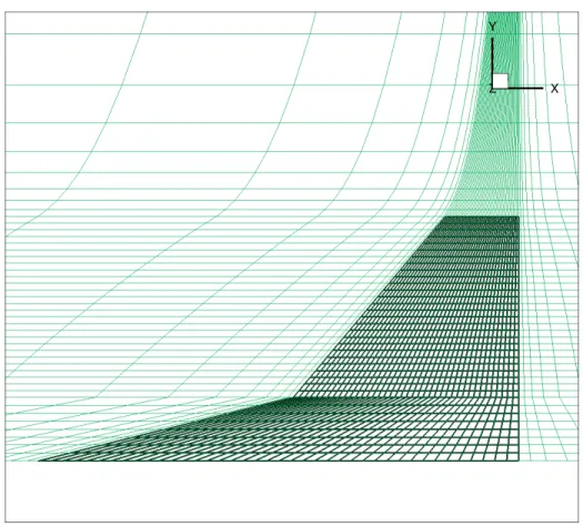
computa-tional mesh. . . 27 3.3 Mesh Generation, Close View. ZEUS uses a built-in, automated

mesh generation scheme to extrapolate a 3-D mesh from the 2-D panel distribution along the wing’s surface. . . 28 3.4 Mesh Generation, Full View. ZEUS uses a built-in, automated mesh

generation scheme to extrapolate a 3-D mesh from the 2-D panel distribution along the wing’s surface. . . 29

3.5 Flow Chart of the Euler Solver in ZEUS. NCYC, NEQTN and

NSTEP refer to input parameters within ZEUS [32]. . . 37 3.6 Dimensioned Top View of Wing. All dimensions on the drawing are

in units of mm. Planform area is equal to 0.144 m2. Chord length is 0.8207 m. Span is 0.435.8 m. . . 40 3.7 3-D View of the computational SiS model at AoA = 4◦. The 4 black

lines on the outer wing section indicate the locations along which Cp was evaluated. The locations denoteCp1, Cp2,Cp3 and Cp4 with

the following physical locations: y = 209 mm, 274 mm, 336 mm and 395 mm from the centerline, respectively. Cp1 is located most

(9)

Figure Page 3.8 Grid Sensitivity. The plot depicts changes in the trim AoA as a

function of panel density for a load factor of 1. The label below each point indicates the number of spanwise and chordwise distributions along the wing, respectively. . . 42 3.9 Aerodynamic Panels on Wing. 1400 panels were created from a

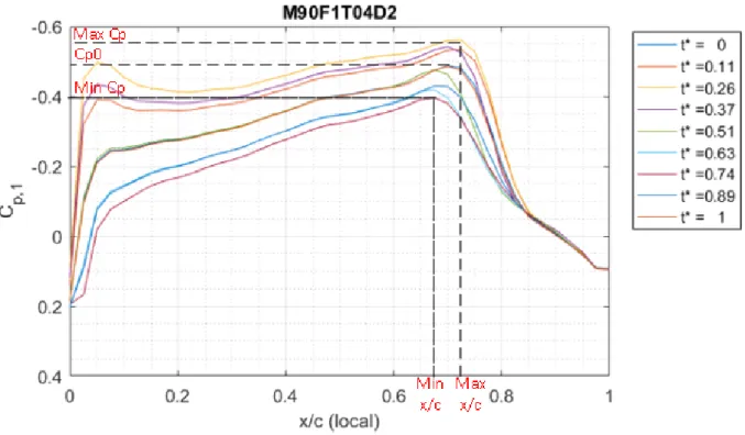
distribution of 41 nodes along the chord and 36 nodes across the span of the Wing. . . 43 4.1 Example figure indicating the min and maxCp and x_c as well as Cp0

for the time trace ofCp1. M = 0.9, Freqeuncy = 5.7 Hz, Trim = 4◦,

∆α = 4◦. . . 48 4.2 Inviscid/Viscous comparison forCp1. M = 0.9, Frequency = 5.7 Hz,

Trim = 4◦. . . 51 4.3 Inviscid/Viscous comparison forCp1. M = 0.9, Frequency = 5.7 Hz,

Trim = 10◦. . . 52 4.4 Inviscid/Viscous comparison forCp4. M = 0.9, Frequency = 5.7 Hz,

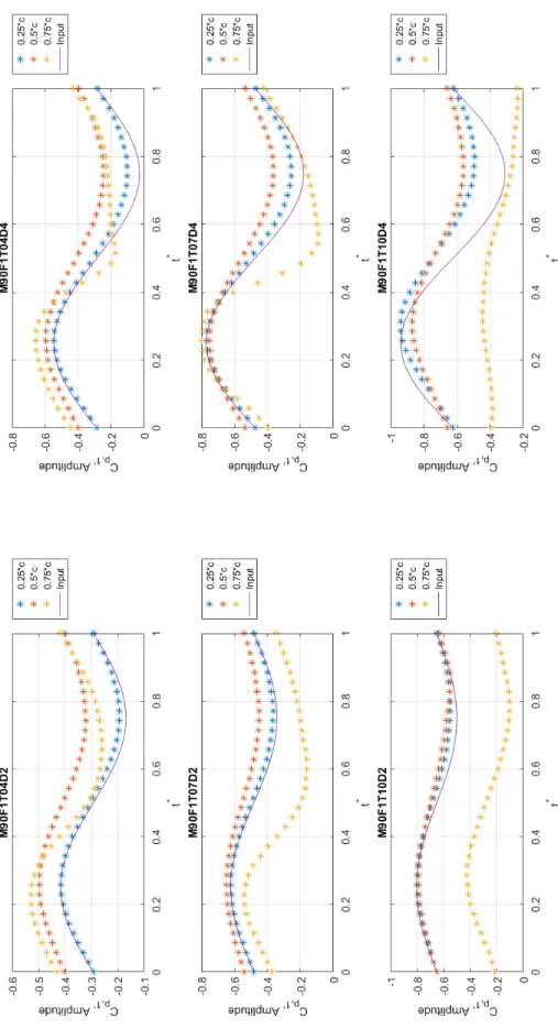
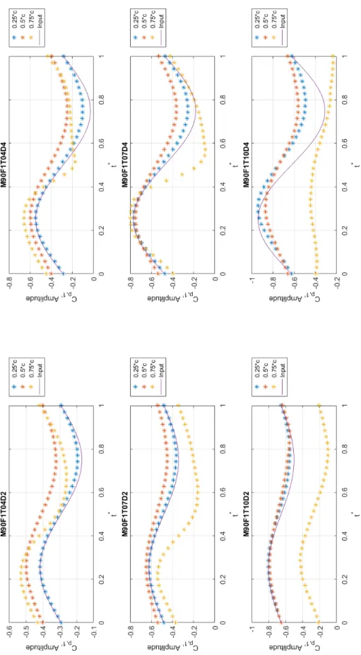
Trim = 7◦. . . 53 4.5 BLC trim and ∆α comparison for Cp1. M = 0.9, Frequency = 5.7 Hz. 55

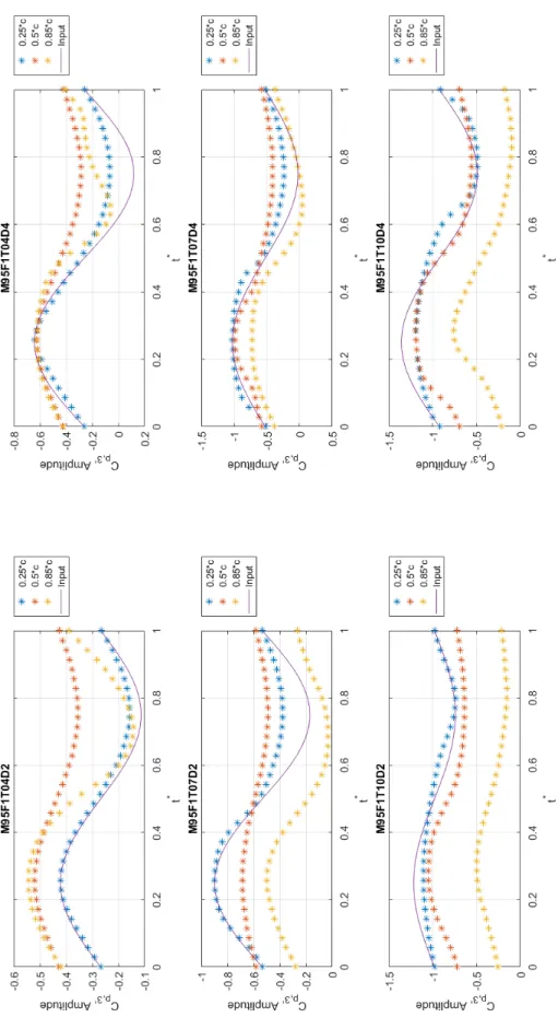
4.6 BLC trim and ∆α comparison for Cp1. M = 0.95, Frequency = 5.7

Hz. . . 56 4.7 BLC frequency comparison for Cp1. M = 0.9, Frequency = 5.7/7.4

Hz. . . 59 4.8 BLC frequency comparison forCp4. M = 0.95, Frequency = 5.7/7.4

Hz. . . 60 4.9 Time history ofCp for three points along the chord of position 1. M

= 0.9, Frequency = 5.7 Hz. . . 61 4.10 Time history ofCp for three points along the chord of position 3. M

= 0.95, Frequency = 5.7 Hz. . . 62 4.11 Time history ofCp for all 4 positions along the wing. The chordwise

position, X, has been normalized by the root chord to retain each position’s relative distance to one another. t∗ = 0.23,0.74 indicate peak nose up and nose down of the wing, respectively. M = 0.9, Frequency = 5.7 Hz, Trim = 4◦, ∆α= 2◦. . . 64

(10)

Figure Page 4.12 Time history ofCp for all 4 positions along the wing. The chordwise

position, X, has been normalized by the root chord to retain each position’s relative distance to one another. t∗ = 0.23,0.74 indicate peak nose up and nose down of the wing, respectively. M = 0.9, Frequency = 5.7 Hz, Trim = 7◦, ∆α= 4◦. . . 65 4.13 Time stamp ofCp whent∗ = 0.0 indicating trimmed position. M =

0.9, Frequency = 5.7 Hz, Trim = 7◦, ∆α= 4◦. . . 66 4.14 Time stamp of Cp when t∗ = 0.0 indicating peak nose up position.

M = 0.9, Frequency = 5.7 Hz, Trim = 7◦, ∆α= 4◦. . . 66 4.15 Time stamp of Cp when t∗ = 0.0 indicating oscillating nose down

past trim. M = 0.9, Frequency = 5.7 Hz, Trim = 7◦, ∆α= 4◦. . . 67 4.16 Time stamp ofCpwhent∗ = 0.0 indicating peak nose down position.

M = 0.9, Frequency = 5.7 Hz, Trim = 7◦, ∆α= 4◦. . . 67 4.17 Variation in the pitching moment coefficient about the quarter-chord

for each wing station over the course of a single oscillation. M = 0.9, Frequency = 5.7 Hz, Trim = 04◦, ∆α =±2◦,±4◦, BLC and Inviscid. 69 4.18 Variation in the pitching moment coefficient about the quarter-chord

for each wing station over the course of a single oscillation. M = 0.9, Frequency = 5.7 Hz, Trim = 07◦, ∆α =±2◦,±4◦, BLC and Inviscid. 70 4.19 Variation in the pitching moment coefficient about the quarter-chord

for each wing station over the course of a single oscillation. M = 0.9, Frequency = 5.7 Hz, Trim = 10◦, ∆α =±2◦,±4◦, BLC and Inviscid. 71 A.1 Frequency Comparison. Time history ofCp for M = 0.90, Frequency

= 5.7 Hz. . . 78 A.2 Frequency Comparison. Time history ofCp for M = 0.90, Frequency

= 7.4 Hz. . . 79 A.3 Time history ofCp for for three points along the chord of station 1.

M = 0.90, Frequency = 5.7 Hz. . . 80 A.4 Time history ofCp for for three points along the chord of station 1.

M = 0.95, Frequency = 5.7 Hz. . . 81 A.5 Mach Comparison. Time history of Cp varying Mach number down

(11)

Figure Page A.6 Mach Comparison. Time history of Cp varying Mach number down

the column. Frequency = 5.7 Hz, Trim = 7◦. . . 83 A.7 BLC trim and ∆α comparison ofCp. M = 0.9, Frequency = 5.7 Hz. 84

A.8 BLC trim and ∆α comparison ofCp. M = 0.95, Frequency = 5.7 Hz. 85

A.9 Inviscid/Viscous comparison of Cp. M = 0.9, Frequency = 5.7 Hz,

Trim = 4◦. . . 86 A.10 Inviscid/Viscous comparison of Cp. M = 0.9, Frequency = 5.7 Hz,

Trim = 7◦. . . 87 A.11 Inviscid/Viscous comparison of Cp. M = 0.9, Frequency = 5.7 Hz,

Trim = 10◦. . . 88 B.1 Frequency Comparison. Time history ofCp for M = 0.90, Frequency

= 5.7 Hz. . . 90 B.2 Frequency Comparison. Time history ofCp for M = 0.90, Frequency

= 7.4 Hz. . . 91 B.3 Time history ofCp for for three points along the chord of station 2.

M = 0.90, Frequency = 5.7 Hz. . . 92 B.4 Time history ofCp for for three points along the chord of station 2.

M = 0.95, Frequency = 5.7 Hz. . . 93 B.5 Mach Comparison. Time history of Cp varying Mach number down

the column. Frequency = 5.7 Hz, Trim = 4◦. . . 94 B.6 Mach Comparison. Time history of Cp varying Mach number down

the column. Frequency = 5.7 Hz, Trim = 7◦. . . 95 B.7 BLC trim and ∆α comparison ofCp. M = 0.9, Frequency = 5.7 Hz. 96

B.8 BLC trim and ∆α comparison ofCp. M = 0.95, Frequency = 5.7 Hz. 97

B.9 Inviscid/Viscous comparison of Cp. M = 0.9, Frequency = 5.7 Hz,

Trim = 4◦. . . 98 B.10 Inviscid/Viscous comparison of Cp. M = 0.9, Frequency = 5.7 Hz,

Trim = 7◦. . . 99 B.11 Inviscid/Viscous comparison of Cp. M = 0.9, Frequency = 5.7 Hz,

(12)

Figure Page C.1 Frequency Comparison. Time history ofCp for M = 0.90, Frequency

= 5.7 Hz. . . 102 C.2 Frequency Comparison. Time history ofCp for M = 0.90, Frequency

= 7.4 Hz. . . 103 C.3 Time history ofCp for for three points along the chord of station 3.

M = 0.90, Frequency = 5.7 Hz. . . 104 C.4 Time history ofCp for for three points along the chord of station 3.

M = 0.95, Frequency = 5.7 Hz. . . 105 C.5 Mach Comparison. Time history of Cp varying Mach number down

the column. Frequency = 5.7 Hz, Trim = 4◦. . . 106 C.6 Mach Comparison. Time history of Cp varying Mach number down

the column. Frequency = 5.7 Hz, Trim = 7◦. . . 107 C.7 BLC trim and ∆α comparison ofCp. M = 0.9, Frequency = 5.7 Hz. 108

C.8 BLC trim and ∆α comparison ofCp. M = 0.95, Frequency = 5.7 Hz. 109

C.9 Inviscid/Viscous comparison of Cp. M = 0.9, Frequency = 5.7 Hz,

Trim = 4◦. . . 110 C.10 Inviscid/Viscous comparison of Cp. M = 0.9, Frequency = 5.7 Hz,

Trim = 7◦. . . 111 C.11 Inviscid/Viscous comparison of Cp. M = 0.9, Frequency = 5.7 Hz,

Trim = 10◦. . . 112 D.1 Frequency Comparison. Time history ofCp for M = 0.90, Frequency

= 5.7 Hz. . . 114 D.2 Frequency Comparison. Time history ofCp for M = 0.90, Frequency

= 7.4 Hz. . . 115 D.3 Time history ofCp for for three points along the chord of station 4.

M = 0.90, Frequency = 5.7 Hz. . . 116 D.4 Time history ofCp for for three points along the chord of station 4.

M = 0.95, Frequency = 5.7 Hz. . . 117 D.5 Mach Comparison. Time history of Cp varying Mach number down

(13)

Figure Page D.6 Mach Comparison. Time history of Cp varying Mach number down

the column. Frequency = 5.7 Hz, Trim = 7◦. . . 119 D.7 BLC trim and ∆α comparison ofCp. M = 0.9, Frequency = 5.7 Hz. 120

D.8 BLC trim and ∆α comparison ofCp. M = 0.95, Frequency = 5.7 Hz. 121

D.9 Inviscid/Viscous comparison of Cp. M = 0.9, Frequency = 5.7 Hz,

Trim = 4◦. . . 122 D.10 Inviscid/Viscous comparison of Cp. M = 0.9, Frequency = 5.7 Hz,

Trim = 7◦. . . 123 D.11 Inviscid/Viscous comparison of Cp. M = 0.9, Frequency = 5.7 Hz,

Trim = 10◦. . . 124 E.1 Cp on the wing’s surface for all 4 chordwise stations. Each plot

indicates a temporal snap shot for the test case: M = 0.90, Frequency = 5.7 Hz, Trim = 4◦, ∆α =±2◦. . . 126 E.2 Cp on the wing’s surface for all 4 chordwise stations. Each plot

indicates a temporal snap shot for the test case: M = 0.90, Frequency = 5.7 Hz, Trim = 10◦, ∆α=±2◦. . . 130 E.6 Cp on the wing’s surface for all 4 chordwise stations. Each plot

indicates a temporal snap shot for the test case: M = 0.90, Frequency = 5.7 Hz, Trim = 10◦, ∆α=±4◦. . . 131

(14)

List of Tables

Table Page

3.1 Test Matrix. The SiS model was run for various combinations of Mach, trim, oscillation amplitude and oscillation frequency. x and o indicate an oscillation frequency of 5.7 Hz and 7.4 Hz, respectively. I indicates a fully inviscid test case. . . 44 4.1 Tabulated Results for cases of interest for position 1 on the wing.

The shock movement is reported in percent of local chord. The per-cent change inCp from the shock migration is reported as (Cp,max− Cp,min)/Cp0 . . . 73

(15)

List of Symbols

Symbol Page M Mass Matrix . . . 6 C Damping Matrix . . . 6 K Stiffness Matrix . . . 6 x Structural Deformation . . . 6 Fa Aerodynamic Forces . . . 6 Fe External Forces . . . 6 q∞ Dynamic Pressure . . . 7

H Aerodynamic Influence Coefficient Matrix . . . 7

(16)

List of Abbreviations

Abbreviation Page

LCO Limit Cycle Oscillation . . . 1

AFSEO Air Force SEEK EAGLE Office . . . 1

AFB Air Force Base . . . 1

SITES Shock Induced Trailing Edge Separation . . . 4

ZEUS ZONA Euler Unsteady Solver . . . 4

EOM Equation of Motion . . . 6

AIC Aerodynamic Influence Coefficient . . . 7

EA Elastic Axis . . . 10

AoA Angle of Attack . . . 13

RANS Reynolds-averaged Navier Stokes . . . 13

TPS Test Pilot School . . . 14

NSD Nonlinear Structural Damping . . . 15

CFD Computational Fluid Dynamics . . . 18

FEM Finite Element Method . . . 26

SBLI Shock Boundary Layer Interaction . . . 48

(17)

An Efficient Euler Method to Predict

Shock Migration on an Oscillating

Straked Delta Wing Design

I. Introduction

As modern threats emerge and evolve, so must the development of new weapon systems. Along with the advent of these new systems, current delivery platforms, such as the multi-role F-16 aircraft, must be able to safely handle and accommodate unforeseen load variations. F-16s are required to achieve both high altitudes and supersonic speeds, which leads to thin airfoil shapes and reduced weight structures. The introduction of heavy loads from newly designed weapon systems compounded with thin, flexible wing structures of the F-16 can result in an aeroelastic instability known as flutter and an aeroelastic nonlinearity known as limit cycle oscillations (LCO). LCO results in undesirable airframe vibrations which can adversely affect pilot performance and degrade targeting accuracy. Additionally, the occurrence of LCO can lead to increased maintenance costs and reduced system lifespan.

The F-16 has nine traditional load stations: a pair of wingtip stations; a pair of underwing missile stations; a pair of generally air-to-ground stations; a pair of inboard stations which can be used to carry external fuel stores; and a centerline station. Due to the ever increasing number of available weapon systems, the total number of possible permutations of load configurations on the F-16 grows. Each of these load configurations must first be certified by the Air Force SEEK EAGLE Office (AFSEO) before the configuration may be flown operationally.

AFSEO is responsible for the test, evaluation, and certification of external equip-ment and munitions carried by Air Force aircraft. As of 1983, AFSEO at Eglin Air Force Base (AFB) has conducted all flutter testing of the F-16. Considering the exten-sive analysis conducted during flight test, it would be impractical to test all available

(18)

load configurations for the numerous flight regimes of the F-16 due to constraints on time, cost and manpower. Thus, computational techniques which emphasize rapid solutions with minimal sacrifice to accuracy are required to identify flutter sensitive configurations [20, p. 1]. Subsequently, only the most critical configurations will re-quire flight test validation. When employed successfully, a computational approach to flight test will lead to reduced costs and expedited fielding of new weapon systems required by the warfighter.

1.1 Background and Motivations

Aeroelasticity is the term used to describe the field of study concerned with the interaction of the aerodynamic forces imposed on an elastic structure in an airstream and the resulting deformation, both statically and dynamically. Classical aerody-namics allows for the prediction of forces on a body given a flow condition. Elasticity is used to determine the deflection of an elastic body under a load. Dynamics in-troduces the effect due to inertial forces. When all three aforementioned fields are applied simultaneously, the process is used to conduct dynamic aeroelastic analysis.

In regards to static aeroelasticity, divergence is an important property which results in catastrophic failure. Divergence occurs when the deformation of a lifting surface serves to increase the aerodynamic load, thus leading to further deformation of the structure; this process continues until complete failure of the structure [18, p. 127]. Flutter is similar to divergence, but it is a dynamic aeroelastic phenomenon. Flutter is a self-excited dynamic instability in which the aerodynamic forces on a flexible body couple with the structure’s natural modes of vibration to produce oscillatory behavior of increasing amplitude [18, p. 175-176]. In general, two or more modes of vibration, such as bending and torsional motion, which under the influence of unsteady aerodynamic forces, interact with each other in such a way that energy is transferred from the passing airstream into the vibrating structure. A special case of nonlinear flutter in which the amplitude of the oscillations remains constant is known as a limit cycle oscillation.

(19)

Figure 1.1: Example of LCO.

Limit cycle oscillations are defined as self-sustained oscillations in which there is a balance between the destabilizing and restoring forces of a system, thus LCO lies on the boundary of instability [22, p. 1]. In regards to aeroelastic LCO, aerodynamic forces are translated into the aircraft’s structure, which in turn deforms due to the applied load. The resultant deformation alters the aerodynamic forces and the process is repeated such that there is a balance between the structural restoring forces and aerodynamic loads. The motion of LCO is unique in that the motion is of limited amplitude, cyclic (motion repeats for a given time period) and oscillatory (vibrational amplitude occurs around some mean value). This means that in its most fundamental state, LCO is defined by sinusoidal motion [2, p. 1]. Figure 1.1 depicts a hypothetical LCO in which some perturbation disturbs the system from rest, resulting in the quasi-steady, nonlinear oscillatory motion of the system attempting to return to equilibrium. The F-16 and F/A-18 are LCO prone at high subsonic and transonic speeds for store configurations with AIM-9 missiles on the wingtips and heavy stores on the outboard pylons. The LCO response is primarily characterized by antisymmetric motion of the wing and stores and lateral motion of the fuselage. In the case of the F-16, LCO occurs at both elevated aircraft load factor maneuvers and level flight, while the vibrations may be self-excited or induced by control inputs. Once initiated, the oscillations perpetuate until flight conditions are altered to a non-LCO prone condition. [2, p. 1].

(20)

The phenomenon of LCO is considered to be closely linked to classical flutter with the exception that the coupling of the unsteady aerodynamic forces and struc-tural response is nonlinear in nature [2, p. 1]. Due to the complicated nature of LCO, the nonlinear differential equations of motion which govern this vibration in-frequently have no analytical solution. Modern computational flutter analyses can accurately predict the frequency of LCO and the predicted flutter speed with zero damping is often quite representative of the LCO onset speed in straight, level flight. When considering more applicable portions of the flight regime such as transonic flight, classical linear flutter analysis techniques fail to predict the onset velocity or amplitude of LCO [10, p. 1].

Amongst aeroelasticians, there is little disagreement that LCO is a product of the nonlinear interaction of the structural and aerodynamic forces acting on the aircraft. However, there is no consensus as to which of these sources is the most signif-icant contributor to the phenomenon. One possible explanation for the occurrence of transonic LCO is the presence of shock induced trailing edge separation (SITES). The role of SITES in limit cycles is thought to act as a nonlinear spring which both triggers and drives LCO [6]. SITES occurs when the flow in the boundary layer separates due to the pressure jump across a shock.

1.2 Research Objectives

The focus of this research is to provide further validation of ZONA Technologies Euler unsteady solver (ZEUS) as a tool to predict the onset and severity of LCO in the F-16. The program used for the flow analysis of the oscillating wing presented in this thesis is an Euler solver with the option to add a coupled boundary layer flow. As an Euler solver, the flow is assumed to be inviscid which raises the question, ”Why use an inviscid solver when the aerodynamic phenomenon of interest is a vis-cous effect?”. Although ZONA’s Euler solver will fail to account for large regions of separation potentially caused by the formation of shocks, the primary interest is the shock movement as a result of wing oscillations.

(21)

ZEUS has been optimized to provide rapid solutions to unsteady flow fields and solutions can be run in a fraction of the time required for a full time-accurate Navier-Stokes solution. With the speed of an Euler solver in mind, ZEUS has the potential to provide predictive flight test capabilities for AFSEO and allow for a faster and more budget-friendly approach to flight test.

At the request of AFOSR project sponsors, the research will compare computa-tional results from ZEUS to previous wind tunnel tests conducted by Cunningham [7] on a half-span straked delta wing design, which closely resembles the F-16’s wing geometry. Cunningham’s tests had the objectives to 1) understand the physics of un-steady transonic vortex flows about a simple straked delta wing and 2) to generate a steady and unsteady airloads data base for a simple straked delta wing to be used for validation of CFD computer codes. For the purposes of this research, a simple straked delta wing was oscillated in pitch for a variety of Mach numbers, trim conditions, os-cillation amplitudes and osos-cillation frequencies in order to closely replicate the wind tunnel experiment and compare the results between the two sources. Additionally, the significance of viscous effects in shock migration was of particular interest. For this reason, fully inviscid and boundary layer coupled solutions were run in parallel to compare any disparities between the two methods.

(22)

II. Literature Review

2.1 Introduction

This chapter will provide an overview from a selection of the computational methods currently employed for aeroelastic analysis in addition to previous research and experiments relevant to limit cycle oscillations. As a precursor to LCO, this section will begin with a review of linear flutter analysis. Next, LCO theory will be discussed along with some of the possible sources of the nonlinear nature of LCO. A brief discussion focusing on AFSEO’s approach to flutter and LCO testing will provide foundation for the motivation behind the author’s research. Finally, the chapter will conclude with an in-depth analysis of Cunningham’s [7] wind tunnel experiment which provides a basis for the author’s own research.

2.2 Fundamentals of Linear Aeroelastic Analysis

Linear aeroelasticity begins with a summation of the forces on a lifting surface in the form of second order equations of motion in matrix form (EOM)

M¨x(t) +C ˙x(t) +Kx(t) = F(t) (2.1)

where M, C, and K are the mass, damping and stiffness matrices, respectively, gen-erated by the structural FEM. The aerodynamic forces acting upon the lifting surface are located on the right hand side of the EOM and can be further defined as

F(t) = Fa(x(t)) +Fe(t) (2.2)

where x represents structural deformation, Fa represents aerodynamic forces, and

Fe(t) represents external forces such as impulse type gust loads, store ejection forces

or control surface deflections due to pilot input [33, p. 2-1]. Should Fa(x(t)) be

nonlinear with respect to time, then a discrete time approach with initial conditions is required.

(23)

To further define the system, dynamic pressure is denoted with q∞ and an

aerodynamic influence coefficient (AIC) withH. We begin recasting (2.1) by assuming no external forces (Fe(t) =0) and that Fa(x) can be interpreted as an aerodynamic

feedback term. Thus the aerodynamic feedback can be related to the structural deformation by way of a convolution integral:

Fa(x(t)) = Z t 0 q∞H L V (t−τ) x(τ)dτ (2.3) where:

q∞H is the aerodynamic transfer function

V is the freestream velocity

τ is the integration variable

and:

L is the reference length, typically half-chord [33].

The Laplace domain analogue of Equation 2.3 is

Fa(x(s)) =q∞H¯(

sL

V )x(s) (2.4)

where:

¯

H is the frequency domain counterpart ofH

s is the complex number frequency parameter

which when combined with (2.1) simplifies to form the eigenproblem:

[s2M¯ +sC¯ +K¯ −q∞H¯(

sL

(24)

The end result of (2.5) is a computationally intensive eigenproblem due to the large size of the mass, damping and stiffness matrices. Common practice makes a simplify-ing assumption that aeroelastic instabilities typically consist of interactsimplify-ing lower-order modes [33]. The “modal approach” truncates the infinite number of modes required for continuous system analysis: 50 natural modes are usually sufficient to conduct analysis of a whole aircraft structure [33, p. 2-3]:

x=Φq in the s-domain (2.6)

whereΦrepresents a modal matrix with only the selected lower order natural modes [33, p. 2-4]. The generalized coordinates, q, is the eigenvector which will be deter-mined. With the eigenvectors in hand, the structural deflections of the airframe are known and then aerodynamic forces can be calculated. With (2.4) and (2.6), the classical flutter matrix equation is produced:

[s2M+sC+K−q∞Q(

sL

V )]q= 0 (2.7)

where:

M = ΦTMΦ¯ is the generalized mass matrix with selected modes

K = ΦTKΦ¯ is the generalized stiffness matrix with selected modes

C = ΦTZΦ¯ is the generalized damping matrix with selected modes

and:

Q(sL

V ) = Φ

T_H_¯₍sL

V )Φ is the generalized aerodynamic forces matrix

The solution process to generate the aerodynamic transfer function with un-steady aerodynamic methods is often facilitated by assuming simple harmonic mo-tion. The frequency domain aerodynamic transfer function in matrix form is called

(25)

the Aerodynamic Influence Coefficient (AIC) [33, p. 2-4]. The formulation of the AIC matrices is the major functionality of ZAERO by way of the g-Method, a flut-ter solution method unique to ZAERO. The g-Method can robustly handle non-zero structural damping and represents the commercial state-of-the-art linear aeroelastic algorithm. Other linear aeroelastic algorithms include the K-Method, P-Method and P-K Method [4].

2.3 LCO Theory

The use of the term LCO in aeroelastic diction has become more prevalent since the 1970s to describe the dynamic response of some aircraft and external store con-figurations to encounter a sustained, oscillatory, periodic, but non-divergent motion within portions of the flight envelope. Historically, terms such as limit cycle flutter and limited amplitude flutter have been used as well. LCO differs from classical flutter primarily in that the nonlinear coupling of aerodynamic and structural forces causes the oscillations to grow from an initial perturbation to some limited amplitude. For typical LCO, the amplitude of the vibrations is constant for a stabilized flight condi-tion. Once above the LCO onset speed, the amplitude of the vibration grows until a new flight speed is achieved. Once the speed is again stabilized, the periodic motion will continue, but at a greater amplitude than the vibrations at lower velocity.

Denegri reported two distinct types of LCO which occurred during the flutter test of the Block 15 F-16A [10]. He classified the two cases of LCO as typical and non-typical LCO. Typical LCO was characterized by a gradual onset of sustained limited amplitude oscillations of the wing where the amplitude increased with increasing Mach number and dynamic pressure. Non-typical LCO was unique in that the oscillations may only be present in a limited portion of the flight envelope.

Although it is easy to recognize the phenomenon, the true source of LCO re-mains shrouded due to the nonlinear nature of this aeroelastic response. Speculation of the root cause of LCO exists, whether it be aerodynamic nonlinearities, structural

(26)

nonlinearities, or a complex interaction of the two. For this reason, classical linear flutter analysis has been shown to adequately predict oscillation frequency and modal composition of the LCO mechanism, but unable to predict the onset speed or severity of the LCO [10, p. 1]. If the source/sources of LCO can be identified, computational models which better predict LCO characteristics can be developed. The following sec-tions will discuss some of the prevailing theories concerning LCO from the perspective of a computational approach.

2.3.1 Store Aerodynamics. Several researchers have observed that many fighter aircraft experience LCO at speeds below the predicted flutter speed when carrying certain combinations of external stores [2, 7, 10, 13, 20, 25, 30]. Stores located under the wing and at the wing tip can affect LCO by altering the inertial properties of the wing or by changing the aerodynamics of the wing. Although the general trends for the addition of store mass in relation to the elastic axis (EA) are established, the role of store aerodynamics in LCO is still under investigation. The EA is a line which spans from the wing root to the wing tip and produces pure bending when a tranverse force is applied or pure torsion when a moment is applied. If store mass is added forward of the EA, the flutter speed generally increases, producing a stabilizing effect, and vice versa for store mass added aft of the EA [19].

It has been hypothesized that store aerodynamics can affect LCO through two primary mechanisms: the store carriage loads transferred into the structure may suf-ficiently change the total forces experienced by the wing or the store could interfere with the airflow on the wing. In a study by Parker, Maple and Beran [25], it was found that store aerodynamics LCO influence are most likely a combination of both mech-anisms. The aerodynamic nonlinearity responsible for LCO in the Goland wing was shock motion and periodic shock formation; stores were added to the underwing and wingtip locations to determine how store aerodynamics affected LCO characteristics. The aerodynamic forces on the store imparted energy into the structure increasing the

(27)

amplitude of LCO while underwing stores interfered with airflow along the bottom of the wing which served to limit the amplitude of LCO.

Several sources indicate that outboard stores and wingtip missiles play a sig-nificant role in LCO characteristics. Bunton found that both the F-16 and F/A-18 encounter LCO at high subsonic and transonic speeds for store configurations with heavy stores on the outboard pylons and AIM-9 missiles loaded on the wingtips [2]. A study by Dubben and Denegri found differences in LCO response characteristics associated with slight aerodynamic differences in underwing missiles [13]. Dubben discovered that slightly longer missiles with a raised collar section for the attachment of fins and canards displayed vastly different LCO response than shorter missiles. Computational analyses suggest that the fin collar has a significant effect on the wing pressure distribution.

A study presented by Hajj and Beran [16] performed higher-order spectral anal-ysis to identify nonlinear aeroelastic phenomena responsible for LCO during a ma-neuver on the F-16. The results from flight test analysis showed that nonlinearities leading to the LCO were mostly present at the forward locations on the wingtip and underwing launchers. The detection of nonlinearities in the launchers and not at the pylon-wing interface indicates that the nonlinearities are associated with the aerodynamic or structural properties of the launcher.

Dowell et al. [15] implemented a nonlinear harmonic balance compressible RANS flow solver to model the unsteady aerodynamics of the F-16 wing. The aerodynamic model consisted of a clean wing with stores and missiles modeled by assuming aerody-namic slender body theory. The structural portion of the aeroelastic model consisted of modal masses and mode shapes obtained from a NASTRAN FEM. The structural inertia and stiffness of the stores were included in the structural model. The focus of his study was to detect any possible aerodynamic nonlinearities coinciding with LCO. Dowell found the flutter onset Mach number to be highly dependent on the geometry of the wing tip. Dowell reached the following conclusions:

(28)

1. An Euler or Navier-Stokes based CFD code is required to predict transonic flutter while a Navier-Stokes code is required for LCO prediction.

2. Correlation between computational results and flight test are highly sensitive to variations in structural frequencies and aerodynamic modeling of wingtip missile fins.

3. LCO frequency and structural modal participation were generally well predicted but mixed results were achieved with LCO amplitude prediction.

Dowell suggests modeling of flow separation on the missile fins and modeling of structural nonlinearities associated with the attachment points between the wing and missiles would lead to possible improvements to future computational methods.

2.3.2 Shock Induced Trailing Edge Separation. In addition to store aerody-namics, it has been proposed that shock induced trailing edge separation (SITES) may play a significant role in LCO characteristics, notably within the transonic regime. When an aircraft reaches its critical Mach number, the flow in some regions is sonic. A normal shock forms and decelerates the flow back to subsonic. Figure 2.1 illustrates the key features of transonic flow on an airfoil.

As the Mach number increases beyond the critical Mach number, a supersonic region forms on the airfoil and is in general terminated by a nearly normal shock, through which the flow is then returned to subsonic. With a further increase of the free stream Mach number, the shock moves aft while the strength of the shock increases. The adverse pressure gradient caused by the pressure jump across the shock can lead to boundary layer separation along the trailing edge. In addition to the changes in the Mach number, small variations in incidence may lead to considerable changes in the pressure distribution, shock position, and shock strength. If the boundary layer downstream of the shock separates completely, the flow can develop an unsteady phenomenon known as buzz. [29].

(29)

Figure 2.1: Flow features on an airfoil at and above the critical Mach number. (Fed-eral Aviation Administration, 2004: 15-7)

The effect of SITES on LCO can be viewed as a feedback loop in which the oscillatory motion of the wing causes the migration of the shock, or the reverse case in which a self-sustained shock oscillation known as shock buffet can lead to vibrations in the wing. The shock oscillation serves to initiate shock buffet, a large-scale flow-induced shock motion which is self-sustained and repeated in an alternating fashion along the upper and lower surfaces of the airfoil. As the angle of attack (AoA) of a wing increases, the shock strength intensifies while moving aft. Once at a sufficiently high AoA, the boundary layer separates either at the foot of the shock or at the trailing edge, leading to a nose-down pitching moment which serves to reduce wing incidence. At some point the flow will reattach and the nose-down moment dissipates. The stored elastic energy within the wing then returns the wing to an elevated AoA and the SITES process is repeated in a cyclic fashion.

Rokoni found that the interaction of shocks formed from transonic flow over a supercritical airfoil with the boundary layer lead to self-sustained shock oscillations and lift fluctuations which results in the initiation of the buffeting phenomenon [26]. Reynolds-averaged Navier Stokes (RANS) equations were utilized to account for the

(30)

strong viscous-inviscid boundary layer interaction behind the shock. This method was used to predict buffet onset and was validated with experimental data.

Cunningham, an advocate of SITES LCO, has suggested that SITES is the non-linear spring which triggers and drives LCO. Cunningham observed that the appear-ance of SITES coincides with the classical trailing edge divergence, a well-established indicator of buffet onset [6]. The role of SITES in LCO was developed in response to the observation that bending mode responses were very well predicted whereas torsion mode responses were consistently underpredicted. The alternating transition from SITES to attached flow could couple with wing torsional motion and low damp-ing, resulting in LCO.

An analysis by Meijer and Cunningham has shown indications that at transonic speeds, SITES plays a dominant role in the development of LCO on a fighter type aircraft [21]. They utilized steady wind tunnel data to develop a LCO prediction method. The method was used to correctly identify several configurations known to encounter LCO. While this semi-empirical technique requires wind-tunnel data for the airframe of interest, their results have the potential to identify aeroelastic instabilities early in the design process of new aircraft.

Due to ease of access and potential for future growth, the majority of the previously mentioned experiments consisted of computational analysis. A study by Tauer [28] combined both computational methods with flight test as part of the Air Force’s Test Pilot School (TPS) program. Tauer sought to use the flight test in order to 1) validate computational methods for use by AFSEO and 2) to identify nonlinear sources of LCO on the F-16 with particular interest in SITES. The flight test used tufting and shadowgraph techniques to conduct in-flight flow visualization. From his flight test, Tauer observed the following:

1. The presence of shocks did not result in any noticeable separation on the tufts. 2. Shock waves did not move in response to the pitching and plunging of the wing

(31)

The movement of shocks on the wing was non-periodic and correlated to changes in flight conditions. For the smaller amplitude LCO experienced during Tauer’s flight test, it appears that some aerodynamic nonlinearity other than SITES is the culprit behind F-16 LCO. Tauer suggested that further analysis of the complex aerodynamics of the underwing with stores may provide insight to the development and sustainment of LCO.

2.3.3 Nonlinear Structural Damping. Within the transonic regime, it is understandable to hypothesize the influence of SITES in LCO characteristics. Despite the plausibility of this hypothesis, LCO is not a phenomenon restricted to transonic flight. A study by Mignolet, Liu, and Chen [23] indicated that a nonlinear transonic aerodynamic model cannot wholly represent the mechanism for wing and store LCO. Rather, a nonlinear structural damping (NSD) model based on Coulomb friction, possibly compounded with nonlinear aerodynamics, would more accurately represent LCO across more of the flight regime instead of just the transonic regime.

NSD can also help to explain why some wind-tunnel tests experience flutter while the matching flight test resulted in LCO. While the aerodynamics should be similar due to matched Reynolds number, the wind tunnel models are constructed of far fewer pieces and components than the full-scale aircraft. The reduced model complexity could result in changes to the NSD which could explain the variation between the wind tunnel test and flight test. A final argument made by Mignolet, Liu, and Chen in support of NSD questions why previous flight tests of four identical F-16s found variations in LCO onset speeds and amplitudes for each aircraft. While the aerodynamics of each aircraft should be the same, unique variations in the structural integrity based on wear patterns from years of use could explain the differences in LCO for each aircraft [23].

Chen has proposed that wing/store LCO is a post-flutter phenomenon which occurs when the flutter mode contains low unstable damping which is identified as a hump mode [5]. Chen goes on to say that the aircraft structure usually contains

(32)

structural nonlinearity such as friction damping. This amplitude-dependent friction damping can limit the growth of the oscillation amplitude resulting in a limited am-plitude steady state oscillation. On the other hand, a typical flutter mode results in amplitude growth largely due to destabilizing negative aerodynamic damping, hence a drastic increase in the damping past the neutral stability point. Chen used his own flutter analysis technique, the g-method, to provide further evdience for NSD by showing a good correlation between the LCO/flutter prediction and the flutter test of the F-16 MA41 and MA43 models [5].

2.3.4 Computational Analysis of LCO. Within the past decades, the use of CFD has become more prevalent in the design and testing of aerospace structures. The use of CFD has also extended into the realm of both steady and unsteady aeroelastic analysis, to include the investigation of flutter and LCO. An aeroelastic study by Nikbay [24] performed both static and dynamic analysis of the HIRENASD wing based on NASA’s reference data to investigate steady and unsteady aeroelastic responses in the transonic regime for low and high Reynolds numbers. The study used the ZEUS Euler solver, the same solver used in the present study.

Nikbay found the ZEUS Euler solver with boundary layer coupling showed some agreement with experimental results and a N-S solver. Due to lower fidelity model-ing of viscous effects, ZEUS overpredicted the shock pressure magnitude, pressure change across the shock and aftward relocation of the shock on the upper surface for the steady case. For the unsteady case, the Euler solution predicts a more aggres-sive dynamic response which occurs further aft than both the RANS solution and experimental results. In general, the Euler solution results agree better with the ex-perimental data sets near the mid-span locations where the effects of the wind tunnel wall boundary layers and wing tip vortices were not as prevalent.

In a vein similar to LCO, shock wave interactions with a separated boundary layer are associated with many unsteady phenomena. For aircraft in flight, flow-induced vibrations known as buffeting can occur when separation of the boundary

(33)

layer occurs. The shock induced fluctuations are often coupled with self-sustained periodic shock motion of varying amplitude, although the mechanisms responsible for the oscillatory motion are not yet fully understood. What is unique about the shock-boundary layer oscillation is that they do not require oscillatory motion of the wing to occur or perpetuate.

Work by Hashimoto et. al. [17] investigated the effects of turbulence model-ing and grid resolution to improve 3-D buffet prediction accuracy with a N-S code. Hashimoto compared two Zonal Detached Eddy Simulations (ZDES) with the Spalart-Allmaras (SA) and Menter’s Shear Stress Transport (SST) models. With the SST model, the shock wave location moved downstream to closely match experimental results, but the shock oscillated widely with a large pressure fluctuation behind the shock. Next, Hashimoto implemented a wall model with ZDES while reducing the number of cells by one-third in order to reduce the computational time required for unsteady simulation. ZDES with the wall model predicted shock wave location and the power spectral density of pressure close to the experiment and in general was able to predict the 3-D buffet reasonably well. As seen by this study, turbulence modeling plays a significant role in N-S codes when predicting transonic shock oscillations due to flow separation.

An alternative to a N-S solution is a boundary layer coupling method. In essence, the procedure involves coupling an outer inviscid region with a inner viscous boundary layer. The coupling method is based on the observation that for transonic flow the unsteady flowfield can be characterized by oscillating shocks and separating and reattaching boundaries. The coupled boundary layer method regards such flow as a simulation of two dynamic systems, the outer inviscid flow and inner viscous boundary, whose coupling requires proper convergence to ensure the coupling error between the two distinct flows is minimized. An in-depth description of this coupling process, called the Edwards method, can be found in the next chapter.

(34)

Edwards [14] used his method to compute the buffet properties for an 18% thick circular arc airfoil for Re = 10E6 and at M = 0.76. The calculated periodic shock frequency agreed closely with the experimental value. Additionally, the coupled boundary layer method was also able to compute the hysteresis effect due to increasing or decreasing Mach number on the onset and quenching of periodic motion quite accurately. For increasing Mach, periodic motion occurs at M = 0.75 compared to 0.76 experimentally while for decreasing Mach, periodic motion quenched at M = 0.735 compared to M = 0.73 experimentally. The increasing Mach number results were more accurate for Edwards method than those obtained by way of a N-S code, although the N-S code did more accurately predict the quenching boundary.

2.4 Current AFSEO Methodology

One of the most problematic conditions with performing LCO analysis is the tremendous volume of analysis cases that must be examined in order to provide cer-tification for a given store configuration and its permutations [12, p. 887]. The ever-increasing cost of flight test compounded with the rapid proliferation of possible flight configurations of an aircraft has led to a considerable growth of AFSEO’s work to clear new weapons and configurations. While typical flutter and LCO analysis only gives an indication of potential flight characteristics, flight test of the most critical configurations is conducted to determine the true LCO characteristics in order to verify the computational analyses.

Computational fluid dynamics (CFD) has become a powerful and accurate tool for aerodynamic analysis and design. Despite the potential of CFD to provide flow solutions for high fidelity full-scale numerical simulations, its ability to efficiently conduct aeroelastic analysis falls short. In order to reliably simulate aerodynamic flow and the associated nonlinear phenomena with the aircraft model requires a significant amount of time. A recent study by Tang showed that using CFL3D required 4 days of computation to complete a transonic LCO study on a 1 GHz computer of 2-D flow over

(35)

an airfoil [27]. Although powerful, the implementation of unsteady CFD to conduct the massive number of aircraft/store configurations for AFSEO is impractical.

AFSEO conducts bulk screening with lower fidelity models to identify flutter-critical or LCO-flutter-critical configurations to offset the high cost of flight test [11, p. 500]. This computational approach to flutter/LCO testing is intended to determine potentially dangerous configurations without the need for testing as well as identify configurations whose response characteristics are acceptable, thus eliminating the need for redundant flight testing [12, p. 887-888]. Given the scope of the problem and available computational resources, AFSEO’s bulk simulations use MSC.NASTRAN’s version of the K-method that includes a low-fidelity aerodynamic model. The F-16 aerodynamic model consists of only 13 panels split into 616 boxes. Aerodynamic modeling of the underwing stores is not included [11, p. 502]. While the aerodynamic model is low fidelity, the F-16 FEM model is the same fidelity as used with other F-16 aeroelastic simulations.

2.5 Straked Delta Wing Wind Tunnel Experiment by Cunningham

Steady and unsteady low speed wing tunnel tests were conducted in 1986 on a pitching simple straked wing model representative of modern fighter aircraft [1,9]. The model was oscillated in pitch at amplitudes sufficient to represent rapid pitch-ups and push-overs at dynamically scaled full scale maneuver times. The tests were used to show how wing and strake vortices develop and interact as well as how they break down and collapse to fully stalled flow. There was interest to extend this understanding to include compressibility effects as well as analysis of LCO flow conditions.

In 1991, Cunningham conducted a combined wind tunnel test using a common instrumented wing panel to investigate configurations at typical LCO flow conditions, and unsteady pressures and forces for a simple straked wing in flow that ranged from incompressible to transonic [7]. The simple straked wing portion of the test had the objective to extend the understanding of flow fields at low speeds and high incidences

(36)

up to transonic speeds and high incidences. The LCO portion of the test had the objective of providing information that could be used to help develop a prediction method for full scale LCO characteristics of elastic aircraft.

The wing test was conducted in the NLR (National Aerospace Laboratory) 2.0 x 1.6 m2 _{high-speed wind tunnel located in Amsterdam. A sidewall mount was used to}

secure the semispan model for a range of Mach numbers spanning from M = 0.225 to M = 0.90. A hydraulic actuator was connected to the turntable which supported the wing balance beam was used to provide oscillatory pitching of the wing. The semispan model was constructed of an aluminum alloy so as to minimize inertial loads. The simple wing/strake (SiS) configuration is shown in Figures 2.2 and 2.3. The outer wing section was a linearly lofted NACA 64A204 with -3◦ of washout at the wingtip. The strake section was attached to the outer wing so that the entire wing oscillated as a single piece.

The model instrumentation included pressure transducers to measure the un-steady pressure coefficient on the wing. Individual pressure ports were located along pressure measurement sections placed both spanwise and chordwise along the wing. Placement of pressure sections can be found on Fig. 2.2. The pressure sections con-sisted of 4 chordwise sections and 3 spanswise sections located on the outer wing. Grouping of pressure transducers toward the wingtip was done to concentrate instru-mentation in the regions of known shock induced separation.

The SiS model was tested at three Mach numbers: M = 0.225, 0.6, and 0.9, all of which were tested at a Reynolds number of 8∗106_{, based on the root chord. The}

wing was then swept from 6◦ to 48◦ of mean incidence with an oscillation amplitude of 0.5◦ to 8◦ at frequencies varying from 5.7 Hz to 15.2 Hz. A sample of the test matrix used by Cunningham can be found in Fig. 2.4. A similar test matrix was used by the author so that the computational results presented in this thesis could be compared to the original wind tunnel tests by Cunningham.

(37)

Figure 2.2: Simple Wing/Strake Configuration. Pressure sensors are located along the dotted lines labled 1-4. (dimensions in mm) [8]

(38)

Figure 2.3: Dimensions of wing panel (dimensions in mm) [8]. The computational model used in this study is slightly different than the model presented here.

(39)

(40)

2.6 Chapter Summary

Within the scope of this literature review, the author has covered the foundation and relevant research pertaining to LCO theory. An introduction covering the linear dynamic unstable aeroelastic response known as flutter explains the transition to the nonlinear response of LCO. Possible sources of LCO such as store aerodynamics, SITES and structural damping were investigated in detail to provide some speculation to the cause of LCO. Current AFSEO flutter/LCO methodology was explained next in order to define the motivation behind alternative computational methods for LCO prediction. Finally, Cunningham’s 1994 Wind Tunnel experiment, which was the basis for the computational study conducted within this investigation, was reviewed.

(41)

III. Methodology

3.1 Introduction

This study performed a series of time-accurate analyses of a wing oscillated in pitch with a commercial Euler code in order to gather data on potential shock migra-tion on the wing. All aeroelastic analysis were carried out with Zona Technologies’ ZEUS software. ZEUS is a commercial Euler Unsteady Aerodynamic Solver which in-volves an automated mesh generation scheme while using a stationary Cartesian grid and implements a boundary layer coupling scheme. ZEUS uses a central difference with JST (Jameson-Schmidt-Turkel) Artificial Dissipation Scheme for flux construc-tion and Green’s Integral Boundary Layer Method to model turbulence. This chapter discusses the Euler method employed and the parameters unique to this study.

3.2 ZEUS

3.2.1 Mesh Generation and Finite Element Model. ZEUS utilizes an auto-mated mesh generation scheme that requires the surface mesh of the lifting surfaces and bodies as input. The automated mesh generation is accomplished by creating a block around the model which defines the outermost boundaries of the three dimen-sional Cartesian mesh. For the purpose of defining the mesh orientation, the origin is located on the root chord with the x, y, and z axis defined as out the tail, laterally out the right wing, and vertically out the top of the aircraft, respectively. The surface grid lines run orthogonally in the X-Y and Y-Z planes. ZEUS then activates a segregation technique that divides the various lifting surfaces into several spanwise zones, called Y-zones. Each aircraft component is projected onto the X-Y plane into individual Y-zones. Within each Y-zone, the leading and trailing edge is extended upstream and downstream, respectively, with the slope of each additional line decreasing so that the final line is parallel to the upstream and downstream X-Y boundary.

A cubic spline technique then extends each line in the Y direction based on the following constraints: the slope of adjoining cells must match and the line must be perpendicular to the X-Z plane at the farfield boundary in the Y direction. The

(42)

Figure 3.1: Mesh Generation, Top View, Close. XY plane view of the computational mesh.

Y-zones allow for ZEUS to build an automated sheared mesh by growing the gridlines from the surface mesh to the outer boundary of the block based on a user defined cell growth rate [32, p. 5-5]. A top-down view of the mesh can be seen in Figures 3.1 and 3.2.

The mesh boundaries were extended two chord lengths upstream, five chord lengths downstream, two spanwidths from the X-Z plane, and a chord length above and below the X-Y plane. The generated mesh can be found in Figures 3.3 and 3.4.

Although various finite element method (FEM) models for the F-16 exist, Cun-ningham’s experiment did not seek to replicate mass/inertial properties of the model wing to a full scale wing. The wing was constructed of aluminum to reduce inertial loads. Impact testing was conducted on the model to determine natural frequencies and vibration modes. The results of these tests allowed for the selection of oscillation

(43)

Figure 3.2: Mesh Generation, Top View, Full. XY plane view of the computational mesh.

frequencies that were not close to the natural frequencies of the model. For harmonic excitation frequencies below 8 Hz, the model was considered rigid. For this reason, it was decided to implement a rigid body computational model with only a rotational pitch mode.

A ”dummy” file was used to define the FEM model which contained a single point located along the strake root at x = 0.733∗Croot. The single point had one

eigenvector which defined rotational pitch mode. All of the aerodynamic panels were then splined to the single FEM point which resulted in rigid body rotational motion of the entire computational model. The entire strake-outboard wing structure was then converted to a control surface with a rotation axis located in the same position as that of the Cunningham model. Treating the entire wing structure as a control surface

(44)

Figure 3.3: Mesh Generation, Close View. ZEUS uses a built-in, automated mesh generation scheme to extrapolate a 3-D mesh from the 2-D panel distri-bution along the wing’s surface.

allowed for direct control of the wing’s orientation so that LCO could be simulated by providing input to the wing to oscillate at a prescribed amplitude and frequency.

ZEUS can run both a full or linearized Euler solver. While ZONA recommends use of the linearized solver when possible, this recommendation applies more-so to small amplitude disturbances. Due to the nonlinear nature of the LCO simulations, high angles of attack, and large oscillation amplitudes, the full Euler solver was uti-lized. ZEUS’ implementation of the Euler solver will be described in a later section.

3.2.2 Unsteady Euler Solver on Stationary Cartesian Grid. ZEUS gener-ates unsteady aerodynamics based on a stationary Cartesian grid. ZEUS solves the time-accurate Euler equations by way of a cell-centered central-differencing

(45)

finite-Figure 3.4: Mesh Generation, Full View. ZEUS uses a built-in, automated mesh gen-eration scheme to extrapolate a 3-D mesh from the 2-D panel distribution along the wing’s surface.

volume method with Jameson-Schmidt-Turkel (JST) artificial dissipation scheme im-plemented for the stability of the flow solver [32, 6.1].

3.2.3 Time-Accurate Euler Method. The three-dimensional Euler equations in conservative differential form and in curvilinear coordinates are as follows:

∂Q ∂t + ∂H1 ∂ξ + ∂H2 ∂η + ∂H3 ∂ζ = 0 (3.1)

where Q is the product of conservative flow variables vector q and the inverse of the transformation Jacobian J, and Hi are the convective fluxes in three curvilinear

(46)

coordinate directions: Q=J q=J            ρ ρu ρv ρw e            H1 =J            ρU ρuU +pξx ρvU +pξy ρwU+pξz (e+p)U−pξt            H2 =J            ρV ρuV +pηx ρvV +pηy ρwV +pηz (e+p)V −pηt            H3 =J            ρW ρuW +pζx ρvW +pζy ρwW +pζz (e+p)W −pζt            (3.2)

U, V, W and u, v, w are the three components of the flow velocity in curvilinear and Cartesian coordinates, respectively, and are related by the following metric terms:

U =ξi·< u, v, w > +ξt V =ηi·< u, v, w >+ηt W =ζi·< u, v, w >+ζt

(3.3)

The gas is assumed to be perfect and the equation of state is:

e= 1

γ−1p+ 1 2ρ(u

2₊_v2₊_w2₎ _(3.4)

Applying Equation (3.1) to each finite-volume grid cell results in a set of ordinary differential equations of the form:

d

dt(qi,j,kΩi, j, k) +R(qi,j,k) = 0 (3.5)

where Ωi,j,k is the volume of the cell with index (i,j,k) and the residual R(qi,j,k) is

(47)

Jameson’s artificial dissipation flux is added to the convective flux for stability:

R(qi,j,k)−Ci,j,k −Di,j,k =Ci,j,k −(D (2) i,j,k−D

(4)

i,j,k) (3.6)

CandDare the flux integrals of the cell due to convective flux and artificial dissipation flux, respectively, while D(2) _and _D(4) _{are the 2nd and 4th order artificial dissipation}

fluxes. Both artificial dissipation fluxes are the sum of the artificial dissipation at all six surfaces of the computational cell. The 2nd and 4th order dissipative terms are defined as: (2)_(i+1 2,j,k) =κ(2)_min_[0_.₂₅_{, max}₍_ν i+1,j,k, νi,j,k)] (4)_(i+1 2,j,k) =maxh0,κ₃₂(4) −(2)_i+1 2,j,k i (3.7)

here κ(2) _and _κ(4) _{are the two parameters VIS2 and VIS4, respectively, found in the}

MKPARAM bulk data card used to control the amount of artificial dissipation present in the Euler solver for stability. The pressure sensor νi,j,k is defined as:

νi,j,k = pi−1,j,k−2pi,j,k+pi+1,j,k pi−1,j,k+ 2pi,j,k+pi+1,j,k (3.8)

The pressure sensor serves as a switch to toggle the effects of the artificial dissipation. In the region close to the shock wave, the pressure has to jump and the value of (2) is of order one which turns on the 2nd order dissipation and disables the 4th order dissipation. Alternatively, in an area with a smooth pressure region, the 2nd order term is turned off and the 4th order dissipation works to damp the high frequencies that the central-differencing scheme fails to damp.

For the time accurate solution, the _dtd operator from Equation 3.5 is approxi-mated by an second-order, implicit backward difference method of the following form:

3 2∆t qn+1Ωn+1− 2 ∆t[q n_Ωn_{] +} 1 2∆t qn−1Ωn−1+R qn+1 = 0 (3.9)

(48)

The equation above can be formed into a steady-state problem with the pseudo time t∗: d(qn+1Ωn+1 dt∗ ) +R ∗ (qn+1) = 0 (3.10) where R∗(qn+1) = 3 2∆t q n+1_Ωn+1 − 2 ∆t(q n_Ωn_{) +} 1 2∆t q n−1_Ωn−1 +R qn+1 (3.11)

A five-stage Runge-Kutta (R-K) pseudo-time marching scheme can be applied to Equation 3.10. A dual-time stepping method is used for the solution of the time-accurate Euler equations due to the two different time-steps, ∆t and ∆t∗. The five-stage R-K pseudo-time marching method is an explicit scheme which limits the pseudo-time step size ∆t∗ to ensure numerical stability. ZEUS uses the Courant-Friedrichs-Lewy (CFL) number to control the size of the time step. The coefficients of the five-stage R-K scheme are chosen such that an optimal CFL number of about 4.0 without residual smoothing can be achieved. If residual smoothing is applied, the maximum attainable value for CFL is pushed up to 8.0. For most practical purposes, ZEUS should be able to use the CFL number of 7.0 for most cases with residual smoothing turned on [32, 6.1].

Due to the implicit method used for the physical time step, the dual-time step-ping method in ZEUS has no limitations on the stability for the physical time step. Therefore, the physical time step should be driven by the flow physics. The ZEUS manual recommends at least 50 physical time steps within a sinusoidal excitation.

ZEUS incorporates a variable-coefficient implicit residual smoothing scheme to further increase the stability range of the Euler solver. In the case of a 2D flow field, the residual smoothing formula is as follows:

(49)

whereRi,j and Ri,j are the residuals before and after smoothing. ∇∆ is the standard

second-difference operator and β is the residual smoothing coefficient. The value of

β can be either a constant or a function of the local spectral radii.

3.2.4 Transpiration Boundary Conditions. For complex configurations, the generation of a body-fitted grid could be a daunting task. Additionally, the use of deforming mesh can cause problems such as grid cross-over or over-skewed mesh when performing unsteady simulations. In order to bypass these issues, ZEUS uses a stationary Cartesian grid by utilizing the transpiration boundary conditions to account for both thickness and small amplitude motion of the wing surface. Due to the stationary grid, all time-derivative based terms from Equations 3.2 such as ξ,

η and ζ are dropped.

A thin wing with slight deformation about its mean position (horizontal plane, z = 0) is then considered. The shape of the upper and lower surfaces of the wing are defined asz =f(x, y) andg(x, y), respectively and the instantaneous position for the upper and lower surfaces are described byz =F(t, x, y) andG(t, x, y). Assuming

||F||<<1, the surface velocity boundary condition on the upper surface of the wing at timet can be found with the first order approximation:

w(t, x, y,0+) = u(t, x, y,0+)Fx+v(t, x, y,0+)Fy+Ft+O(F) (3.13)

The subscripts x, y and t indicate partial derivatives;O(F) represents terms with the same order of magnitude asF or higher. The normal velocity boundary condition on the lower surface is treated in a similar fashion.

The normal momentum equation is used to derive the boundary condition for pressure: ~ n· " ∂ ~V ∂t + ( ~ V · ∇)V~ # =~n· −∇p ρ (3.14)

whereV~ is the flow velocity and~nis the unit normal at the wing surface. The pressure gradient in the normal direction can be derived from the previous equation for the

(50)

upper surface of the wing.

pz(t, x, y,0+) =px(t, x, y,0+)Fx+py(t, x, y,0+)Fy− ρ(Ftt+ 2Ftxu+ 2Ftyv+ 2Fxyuv+Fxxu2+Fyyv2) +O(F)

(3.15)

Further details regarding the application of a stationary Cartesian grid to this Euler unsteady method can be found in Zhang [31].

3.2.5 Boundary Layer Coupling. In order to circumvent the need to develop a complex RANS solver for a Cartesian grid, ZEUS provides a boundary layer coupling scheme which accounts for the viscous effects associated with aerodynamic flows of general concern. When considering flows with relatively high Reynolds number in the millions, the boundary layer is confined to a thin space along the surface. This assumption allows the flow to be partitioned into two zones: a viscous boundary layer while the rest of the flow can be treated as inviscid. For the solution of the boundary layer, an integral method or finite difference method are available. Due to the complexity and uncertainties associated with accurately modeling turbulence with a finite difference method, an integral boundary layer method was chosen to be coupled with the ZEUS (Euler) solver.

3.2.6 Integral Boundary Layer Method. The integral boundary layer method is applied in a 2-D quasi-steady manner; the boundary layer parameters are solved in-dependently at each physical time step in the freestream x direction and then coupled with the inviscid Euler flow solution for each individual strip in the y direction. The quantities of the integral boundary layer are governed by the following set of ordinary differential equations: dUv e dx =F1+F2 1 m dm dx dH dx =F3+F4 1 m dm dx dCE dx =F5 +F6 dUi e dx (3.16)