Learning dispatching rules via an association rule mining approach

(1)

2015

Learning dispatching rules via an association rule

mining approach

Dongwook Kim Iowa State University

Follow this and additional works at:https://lib.dr.iastate.edu/etd Part of theEngineering Commons

This Thesis is brought to you for free and open access by the Iowa State University Capstones, Theses and Dissertations at Iowa State University Digital Repository. It has been accepted for inclusion in Graduate Theses and Dissertations by an authorized administrator of Iowa State University Digital Repository. For more information, please contactdigirep@iastate.edu.

Recommended Citation

Kim, Dongwook, "Learning dispatching rules via an association rule mining approach" (2015).Graduate Theses and Dissertations. 14383.

(2)

Learning dispatching rules via an association rule mining approach

by

Dongwook Kim

A thesis submitted to the graduate faculty

in partial fulfillment of the requirements for the degree of MASTER OF SCIENCE

Major: Industrial Engineering Program of Study Committee: Sigurdur Olafsson, Major Professor

Guiping Hu Heike Hofmann

Iowa State University Ames, Iowa

2015

(3)

TABLE OF CONTENTS Page LIST OF FIGURES ... iv LIST OF TABLES ... v ACKNOWLEDGEMENTS………. ... vii ABSTRACT………. ... viii CHAPTER 1 INTRODUCTION ... 1 1.1 Motivation ... 1 1.2 Objective ... 2 1.2 Thesis Organization ... 2

CHAPTER 2 LITERATURE REVIEW ... 4

CHAPTER 3 METHODOLOGY ... 7

3.1 Single Machine Scheduling Problem ... 7

3.2 Data Mining: Classification and Decision Tree ... 8

3.3 Data Mining: Association Rule Mining ... 9

CHAPTER 4 SINGLE MACHINE SCHEDULING APPLICATION ... 11

4.1. Discovering Longest Processing Time (LPT) First Rule ... 11

4.2. Discovering Earliest Due Date (EDD) First Rule ... 16

4.3. Discovering Weighted Shortest Processing Time (WSPT) First Rule ... 21

4.4. Discovering Weighted Earliest Due Date (WEDD) First Rule ... 25

CHAPTER 5 JOB SHOP SCHEDULING APPLICATION ... 31

5.1. Discovering Scheduling Rules for Machine 1 ... 33

(4)

REFERENCES ... 51 APPENDIX A

(5)

LIST OF FIGURES

Page

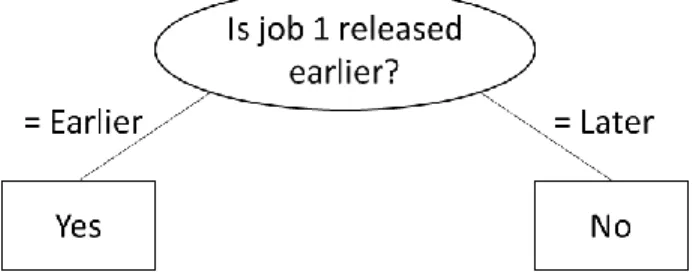
Figure 1 Decision tree classifying the training set of Table 3 ... 13

Figure 2 Graphical analysis for identifying strong associations: EDD rule ... 20

Figure 3 Graphical analysis for identifying strong associations: WSPT rule ... 24

Figure 4 Graphical analysis for identifying strong associations: WEDD rule ... 29

Figure 5 Graphical analysis for identifying strong associations: machine 1 ... 35

(6)

LIST OF TABLES

Page Table 1 List of research on the data mining application to scheduling,

from 2011 to 2015 ... 5

Table 2 Job sequence by Longest Processing Time (LPT) first rule ... 12

Table 3 The training set generated from the job schedule by LPT rule ... 13

Table 4 Gain ratio of attributes in the training set of Table 3 ... 14

Table 5 Association rules generated from the schedule by LPT rule ... 15

Table 6 The first set of core scheduling information: LPT rule ... 16

Table 7 The second set of core scheduling information: LPT rule ... 16

Table 8 Job sequence by Earliest Due Date (EDD) first rule ... 17

Table 9 Association rules generated from the schedule by EDD rule ... 19

Table 10 The first set of core scheduling information: EDD rule ... 21

Table 11 The second set of core scheduling information: EDD rule ... 21

Table 12 Job sequence by Weighted Shortest Processing Time (WSPT) first rule .. 22

Table 13 Association rules generated from the schedule by WSPT rule ... 23

Table 14 The first set of core scheduling information: WSPT rule ... 25

Table 15 The second set of core scheduling information: WSPT rule ... 25

Table 16 Job sequence by Weighted Earliest Due Date (WEDD) first rule ... 26

Table 17 Association rules generated from the schedule by WEDD rule ... 28

Table 18 The first set of core scheduling information: WEDD rule ... 30

Table 19 The second set of core scheduling information: WEDD rule ... 45

(7)

Table 21 The training set derived from the schedule of machine 1 ... 33

Table 22 Association rules generated from the schedule of machine 1 ... 34

Table 23 The first set of core scheduling information: Machine 1 ... 35

Table 24 The second set of core scheduling information: Machine 1 ... 36

(8)

ACKNOLWDGEMENTS

I would like to take this opportunity to express my thanks to those who helped me with various aspects of conducting research and the writing of this thesis. First of all, I would like to thank my advisor, Dr. Sigurdur Olafsson for his constant assistance throughout this research and the writing of this thesis. Whenever I lost confidence, his insights and words of encouragement helped me improve and complete this work. I deeply appreciate his support during my study. I would also like to thank my committee members for their efforts and contributions to this work: Dr. Guiping Hu and Dr. Heike Hofmann.

(9)

ABSTRACT

This thesis proposes a new idea using association rule mining-based approach for discovering dispatching rules in production data. Decision trees have previously been used for the same purpose of finding dispatching rules. However, the nature of the decision tree as a classification method may cause incomplete discovery of dispatching rules, which can be complemented by association rule mining approach. Thus, the hidden dispatching rules can be detected in the use of association rule mining method. Numerical examples of scheduling problems are presented to illustrate all of our results. In those examples, the schedule data of single machine system is analyzed by decision tree and association rule mining, and findings of two learning methods are compared as well. Furthermore, association rule mining

technique is applied to generate dispatching principles in a 6 x 6 job shop scheduling

problem. This means our idea can be applicable to not only single machine systems, but also other ranges of scheduling problems with multiple machines. The insight gained provides the knowledge that can be used to make a scheduling decision in the future.

(10)

CHAPTER 1 INTRODUCTION

1.1 Motivation

Scheduling refers to activities of decision-making in manufacturing systems; generally, a scheduling problem can be defined as the work that properly allocates limited resources to tasks [1]. In order to solve those scheduling problems, many mathematical theories have been

developed and presented for a long time. However, scheduling problems in practice are

somewhat different from the theoretical models; well-developed theories are often inapplicable in real-world scheduling problem due to the problems’ complexity [2]. In such real production environments, scheduling problems would be solved not by mathematical theories, but instant decisions by a production manager. When there is such an expert scheduler, it would be worthwhile to learn from his or her scheduling expertise. Other managers can utilize such knowledge for scheduling in the future without the assistance of the expert scheduler.

These days huge amount of data is generated during manufacturing processes such as scheduling, product design and quality control. Naturally, the ability to efficiently utilize large data becomes a key factor for successful production management. In the view of the importance of data utilization, industries and academic fields have paid attention to data mining techniques. One strength of data mining is that it enables us to find meaningful information in a large data set. Therefore, hidden information could be detected by data mining techniques. When it is difficult to mathematically formulate a production expert’s knowledge on scheduling models, data mining techniques could be used to capture and learn the expert scheduler’s skills.

(11)

1.2 Objective

As mentioned in previous section, an expert scheduler plays an important role in solving real-world scheduling problems. Thus we assume that it is important to learn and share the expertise of the scheduler. Similar to the assumption of our study, Li and Olafsson [3] used a data mining technique for leaning a human scheduler’s expertise. In their study, decision tree method was applied to former production data to learn how a human scheduler made a

scheduling decision. The result or a tree-shaped classification model indicated decision rules that the scheduler followed. However, decision tree technique may find incomplete scheduling knowledge due to the characteristic of the technique; some information might be unrevealed during decision tree learning. If we miss some parts of scheduling knowledge, it would be hard to use the knowledge in the future. For complete discovery of scheduling knowledge, it is necessary to consider another data mining technique as a complement to decision tree method.

The objective of this study is to discover the hidden scheduling knowledge that decision tree technique fails to find, by another type of data mining method called association rule mining. For this objective, historical production data is analyzed by two respective data mining techniques: decision tree and association rule mining. Then, findings from those two methods will be compared. We aim at showing that association rule mining technique discovers

scheduling insights that were unrevealed in the use of other data mining methods.

1.3 Thesis Organization

This thesis is organized as follows. Chapter 2 reviews previous studies related to our topic for showing the originality of this thesis. Chapter 3 explains the methodologies that we follow; concepts of a scheduling model and data mining techniques are introduced. Chapter 4

(12)

and 5 discuss how our idea is actually performed. Illustrative examples of two well-known scheduling environments, single machine and job shop, respectively, are provided. Then lastly, chapter 6 summarizes overall results and implications along with future direction of research.

(13)

CHAPTER 2 LITERATURE REVIEW

Data mining techniques have been applied to production scheduling area for the purpose of knowledge discovery for the last two decades. In an early work, Nakasuka and Yoshida [4] employed machine learning technique for capturing scheduling knowledge. They collected empirical data by simulating iterative production line, then a binary tree was generated from the empirical data. The binary tree determined which scheduling principle was used at decision time during the actual production operations.

In another early work, Yoshida and Touzaki [5] used apriori algorithm to evaluate the usefulness of dispatching rules in complex manufacturing systems. In their work a job shop scheduling problem under two performance measures was solved by some simple dispatching rules such as Earliest Due Date (EDD) and Shortest Processing Time (SPT) first rules. Then, apriori algorithm was used to find associations between performance measures and dispatching rules; associations are expressed as the form, {performance measure} ⇒ {dispatching rules}. The association with the highest support was selected as the best dispatching rule under the

performance measure.

The concept of above studies was selecting between dispatching rules. Those dispatching rules were previously known to us. Unlike this concept, in a work of Li and Olafsson [3] a data mining technique generated or discovered dispatching rules from earlier production data. The dispatching rules generated were formerly unknown to us. In their work, the earlier production data was first transformed into an appropriate form, so that the production data can be analyzed by C4.5 decision tree algorithm. Then, decision tree algorithm discovered dispatching rules that

(14)

were actually used for the schedule shown in the production data. However, in their work there was a possibility that decision tree algorithm learned from imperfect scheduling practices as well as best scheduling practices. The dispatching rule from imperfect scheduling practices would result in low schedule performance. In a later extension of the work, Olafsson and Li [6] improved this shortcoming by using genetic algorithm. Between high and low quality of

scheduling practices in a production data set, high quality scheduling cases were only selected by genetic algorithm. As a result, it was possible for decision tree algorithm to learn from optimal production data.

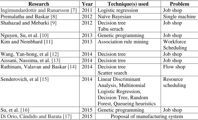
There are also many other studies with respect to the data mining application on scheduling. Some of the studies in recent five years are summarized in Table 1.

Table 1. List of research on the data mining application to scheduling, from 2011 to 2015.

Research Year Technique(s) used Problem

Ingimundardottir and Runarsson [7] 2011 Logistic regression Job shop

Premalatha and Baskar [8] 2012 Naïve Bayesian Single machine Shahazad and Mebarki [9] 2012 Decision tree

Tabu serach

Job shop Nguyen, Su, et al. [10] 2013 Genetic programming Job shop Kim and Nembhard [11] 2013 Association rule mining Workforce

Scheduling Wang, Yan-hong, et al [12] 2014 Decision tree Job shop Aissani, Nassima, et al. [13] 2014 Decision tree Job shop Rathinam, Valavan and Baskar [14] 2014 Decision tree

Scatter search

Flow shop Senderovich, et al [15] 2014 Linear Discriminant

Analysis, Multinomial Logistic Regression, Decision Tree, Random Forest, Queueing heuristics

Resource scheduling

Su, et al. [16] 2015 Genetic programming Job shop

(15)

This sampling of recent works shows that decision tree technique has been a popular in the field of intelligent scheduling. There are also a few studies adopting other techniques besides decision trees. For example, Kim and Nembhard [11] applied association rule mining technique to

workforce scheduling. In the sense that association rule mining method is used, there might be a similarity between their work and this thesis. However, we focus association rule mining

application on finding unique information that is hidden in the use of other data mining

techniques. Also, we employ single machine and job shop environments as test problems, which is different from the workforce scheduling. To the best of our knowledge, our association rule mining approach as a complement to other data mining techniques has not been studied in intelligent scheduling area.

(16)

CHAPTER 3 METHODOLOGY

3.1 Single Machine Scheduling Problem

The scheduling in single machine environments can be referred as a problem that allocates a set of jobs to one machine. Each of the jobs (for example, job j) has its own specific attributes such as processing time (𝑝_𝑗), release time (𝑟_𝑗), due date (𝑑_𝑗), and weight (𝑤_𝑗). The completion time (𝐶𝑗) of job j indicates the end time when the job finishes its processing. Single

machine scheduling problem is solved by placing jobs in order according to the specific

objectives. For example, a production manager may want to schedule all jobs before due date as early as possible. In this case the objective of the scheduling depends on jobs’ due date. In other words, the scheduler wants to minimize the maximum lateness. The lateness of job j is defined as

𝐿𝑗 = 𝐶𝑗 − 𝑑𝑗.

Also, the maximum lateness is defined as

𝐿𝑚𝑎𝑥 = max(𝐿1, … , 𝐿𝑛).

Theoretically, the maximum lateness is minimized by dispatching jobs in increasing order of due date [1].

The premise of this thesis is that a single machine scheduling problem is solved by an expert scheduler’s intuition, rather than theoretical dispatching rules due to complex production environments. Therefore, our task is to discover the scheduling principle of the scheduler by using data mining techniques. Following sections will introduce concepts of data mining.

(17)

3.2 Data Mining: Classification and Decision Tree

Classification can be referred to a task of data analysis [18]. A data set used for

classification includes a special column, namely, a class attribute, which categorizes instances as a specific value.

Usually, classification follows two processes: learning and classification steps. First, in learning stage, a data set with a class attribute, namely, a training set is given. Then, the training set is analyzed by a specific classification algorithm. As a result, a classifier or classification model is generated. Second, in classification stage, the classification model constructed in learning stage is used to categorize new data set where the class value is unlabeled. Also, the classification model reports the key point of a data set, patterns and rules hidden in the data set.

A single machine scheduling problem can also be considered as a classification task. When two jobs, job 1 and job 2 are given, we want to know which job is dispatched earlier than another one. In this case a class attribute corresponds to “Job 1 goes first”, and this attribute would take a “Yes” value if job 1 is allocated earlier than job 2. On the contrary, if job 2 is assigned faster than job 1, the class attribute “Job 1 goes first” would categorize as “No”. In this way, it is possible to transform a job schedule into a training set with a class attribute, so that classification can be applied. By learning from the training set, we can induce which pattern allows a job to be scheduled first; scheduling rules can be extracted from the classification model corresponding the training set of a job schedule.

In this thesis, we use a decision tree classifier called C4.5 algorithm [19] to induce scheduling rules from scheduling data. Decision tree is one of the most widely-used data mining methods to find hidden patterns in a data set. The result of the method, namely, a tree-shaped classification model is highly straightforward to understand; we can directly interpret the model.

(18)

However, insignificant attributes may not be seen in the output of decision tree algorithm. The algorithm selects the most important attribute as a top tree node. Then, the second important attribute is chosen as a second level of node, and so forth. C4.5 algorithm employs gain ratio to measure the importance of attributes. If a decision tree is split by the attribute with a large

number of gain ratio, the tree would clearly classify corresponding data set, and vice versa. Thus, decision tree algorithm tends to ignore attributes with a small gain ratio for constructing a simple tree. Considering such a feature of decision tree algorithm, there is a possibility that some

information may not be detected with this learning method.

3.3 Data Mining: Association Rule Mining

When decision tree algorithm fails to discover particular scheduling rules, another type of data mining approach, namely, unsupervised learning can be considered to reveal the particular rules. Unsupervised learning is different from classification or supervised learning in the sense that the data set of unsupervised learning does not have a class attribute. One of the most famous unsupervised learning methods is association rule mining. This method searches interesting correlations called association rules between any attributes in the data set. Thus, some specific rules that decision tree missed could possibly be discovered with the association rule mining technique. An association rule generated is expressed as the form, ‘A ⇒ B’, where A and B are the antecedent and consequent parts of the association rule, respectively. For example, an association rule can be interpreted as ‘If job 1 processing time is longer than job 2, then job 1 goes first.’ In this research, we employ apriori algorithm [20], which is the most frequently used association rule mining method.

(19)

Association rule mining technique generates a number of association rules. It is necessary to evaluate the quality of the association rules, so that we can obtain only important and useful information. In general, the quality or interestingness of an association rule can be evaluated by the following three measures: support, confidence, and lift. Support is the proportion of instances in a data set containing both the antecedent and consequent parts of the rule. The support of an association rule, ‘A ⇒ B’is defined as below:

𝑆𝑢𝑝𝑝𝑜𝑟𝑡(𝐴 ⇒ 𝐵) = 𝑃(𝐴 ∩ 𝐵).

Confidence is a probability that the consequent part of a rule occurs when the condition that the antecedent part of the rule occurs is given. The confidence of an association rule, ‘A ⇒ B’ can be calculated as follows:

𝐶𝑜𝑛𝑓𝑖𝑑𝑒𝑛𝑐𝑒(𝐴 ⇒ 𝐵) = 𝑃(𝐵|𝐴) = 𝑃(𝐴 ∩ 𝐵) 𝑃(𝐴) .

Lift is the ratio of the observed support to that expected if the antecedent part and consequent part of a rule were independent. The lift of an association rule, ‘A ⇒ B’ is given by:

𝐿𝑖𝑓𝑡(𝐴 ⇒ 𝐵) = 𝑃(𝐴 ∩ 𝐵) 𝑃(𝐴) ∙ 𝑃(𝐵).

This measure reflects the correlation of the rule. If the occurrence of the antecedent part of the rule is negatively correlated with the occurrence of B, the lift of the rule is less than 1, and vice versa. Hence, we are interested in the rules where lift is over 1.

A user specifies the minimum level of the three measures. Association rules satisfying the minimum level of the measures can be identified as strong association rules, which will provide us with meaningful information. However, all the strong association rules might not be useful. That is, there are redundant information in the set of the strong rules. Therefore, it is also required to prune and group those rules, so that only important information can be extracted.

(20)

CHAPTER 4

SINGLE MACHINE SCHEDULING APPLICATION

In this chapter, four numerical examples will illustrate that how an association rule mining-based approach from a former schedule discovers the hidden dispatching rules that decision tree method previously missed. All of those examples use a single machine scheduling problem with specific objective and corresponding dispatching rules.

4.1 Discovering Longest Processing Time (LPT) First Rule

Longest Processing Time (LPT) first rule sequences jobs in decreasing order of processing times; for all released jobs, the one with longer processing time is first scheduled. Generally, this rule is applied in parallel machines environment when we want to balance the workload over the machines [1]. Now the first illustrative example is solved by the LPT rule, and corresponding solution or schedule is illustrated in Table 2. Suppose that we do not know what dispatching rule is actually used, so we want to induce the dispatching rule from the given schedule by data mining techniques.

(21)

Table 2. Job sequence by Longest Processing Time (LPT) first rule Job No. 𝑟_𝑖 𝑝_𝑖 𝐶_𝑖 7 0 9 9 4 9 3 12 3 11 7 19 1 19 6 25 2 23 6 31 10 30 10 41 9 36 9 50 6 20 5 55 5 29 4 59 8 40 2 61

The first step for using learning methods such as decision trees is to construct a training data set with a class attribute. The dispatching list of Table 2 is currently unsuitable for applying decision tree method. Hence, it is required to transform the dispatching list into a training set. Similarly, Li and Olafsson [3] generated a training set stemmed from historical schedule. In their training set, every job was compared in pairs. Then, a class attribute determined which job is first dispatched. We also follow their approach to convert dispatching list into a training set. Table 3 indicates the training set derived from the dispatching list of Table 2. As it can be seen in Table 3, all jobs, from job 1 to job 10, are examined pairwise, and the last class attribute “Job 1 First” decides which job should be allocated ahead of another. There are also two newly created attributes: “Job 1 RT” and “Job 1 PT”. Those two attributes inspect which job has larger or smaller value of release time and processing time, respectively. This sort of attribute creation is highly necessary to gain a transparent decision model [3]. Accordingly, the training data set can be analyzed by data mining methods.

(22)

Table 3. The training set generated from the job schedule by LPT rule. Job 1 𝑟₁ 𝑝₁ Job 2 𝑟₂ 𝑝₂ Job 1

RT

Job 1 PT

Job 1 First

1 19 6 2 23 6 Earlier Same Yes

1 19 6 3 11 7 Later Shorter No

1 19 6 4 9 3 Later Longer No

1 19 6 5 38 4 Earlier Longer Yes

. . . .

8 40 2 10 30 10 Later Shorter No 9 36 9 10 30 10 Later Shorter No

As a first learning method, C4.5 decision tree algorithm analyzes the training data of Table 3. As mentioned in previous chapter, decision tree algorithm constructs a tree-shaped classification model as a result. Figure 1 displays this tree-shaped classification model, which corresponds to the scheduling rule. According to this rule, a job with earlier release time is allocated first than the later one. As shown in the schedule of Table 2, actually, the first six jobs are dispatched in ascending order of release times. However, it can also be seen that the last four jobs are assigned based on processing times, which is the actual principle adopted. Despite this, a processing time-related rule is not seen in the output of C4.5 algorithm.

(23)

The C4.5 decision tree algorithm uses gain ratio as an attribute selection criteria. The attribute with large gain ratio is selected as a node, whereas the smaller one might not be chosen as a node. Table 4 shows gain ratios of the attributes in the training data. According to the table, “Job 1 RT” attribute has the highest value, so the attribute becomes a sole top node, which can be seen in the decision tree of Figure 1. This means that by selecting “Job 1 RT” attribute as a sole node, C4.5 algorithm can construct more transparent tree; if other attributes with smaller gain ratios are selected, the tree would not be simple and transparent. Gain ratios of “𝑝₂”, “Job 1 PT”, and “𝑝₁” attributes, which are related to processing time, are relatively small, so C4.5 algorithm ignored those attributes, which cannot be seen in the decision tree of Figure 1.

Table 4. Gain ratios of attributes in the training set of Table 3 Rank Attribute Gain ratio

1 Job1 RT 0.649 2 𝑟₂ 0.483 3 𝑝₂ 0.221 4 Job 1 PT 0.128 5 𝑝₁ 0 6 𝑟₁ 0

If we want to find a processing time-related rule, following learning method would be able to consider all attributes, so that they are included in the output. Such a requirement leads to the adoption of apriori association rule mining algorithm. The advantage of this algorithm is that every attribute has the same importance with the algorithm, so it searches association rules between any attributes including the one related to processing time.

Association rule mining method is designed for the analysis of categorical data, so numerical data cannot be analyzed. Therefore, we exclude numerical attributes from the training

(24)

set of Table 3; the last three categorical attributes are used as a new training set for using apriori algorithm. Table 5 reports the output of apriori algorithm.

Table 5. Association rules generated from the schedule by LPT rule Rule No. Job 1 R.T. Job 1 P.T. _⇒ Job 1

First Supp. Conf. Lift

Found by D.T.?

1 Later Shorter ⇒ No 0.31 1 2.37

2 Earlier Longer ⇒ Yes 0.27 1 1.73

3 Later ⇒ No 0.38 0.94 2.24 Yes

4 Earlier ⇒ Yes 0.56 0.93 1.60 Yes

5 Earlier Shorter ⇒ Yes 0.29 0.85 1.46

6 Longer ⇒ Yes 0.36 0.81 1.41

7 Shorter ⇒ No 0.24 0.59 1.40

As it can be seen above, the most notable finding is LPT principle (rule 1, 2, 6 and 7); for the released job, the one with longer processing time is scheduled first. In particular, the highest confidence of the first two rules verifies the accuracy of the LPT principle. Also, we can see a release time related-rule (rule 4 and 5). This is the same as the output of decision tree algorithm. On the other hand, there is an exceptional finding which is against the LPT rule (rule 5); in this rule, a job is first scheduled in spite of its earlier release and shorter processing times. For example, in the schedule of Table 2, job 1 has earlier release and shorter processing times than job 10. When job 1 is dispatched, job 10 is not released. Hence, the exceptional case is due to release time. However, for the released jobs, LPT principle is applied without exception. This can be confirmed in the last four jobs in Table 2.

We select two sets of the core scheduling information from all the association rules listed in Table 5. The first set, where rules correspond to earlier release time first rule, is reported in Table 6. The rules in this table have significantly higher support and confidence than any others.

(25)

For example, rule 4 occurs in 56% of all instances in this scheduling data. In addition, according to the support of the rule, for 93% of the times a job has earlier release time the job is scheduled first as well. This dominance of the rule leads that the decision tree algorithm discovers the result. The second set, where rules indicate LPT principle, is reported in Table 7. This set of rules is a novel finding, which can only be observed in the association rule mining application. Also, both rules in the table have confidence of 100%. In other words, whenever a job has earlier release and longer processing times, the job is scheduled first with the certainty of 100%.

Table 6. The first set of core scheduling information: LPT rule Rule No. Job 1 R.T. Job 1 P.T. _⇒ Job 1

Found by D.T.?

3 Later ⇒ No 0.38 0.94 2.24 Yes

4 Earlier ⇒ Yes 0.56 0.93 1.60 Yes

Table 7. The second set of core scheduling information: LPT rule Rule No. Job 1 RT Job 1 PT _⇒ Job 1

Found by DT?

1 Later Shorter ⇒ No 0.31 1 2.37

2 Earlier Longer ⇒ Yes 0.27 1 1.73

4.2 Discovering Earliest Due Date (EDD) First Rule

As mentioned in the previous chapter, when the objective of scheduling is to minimize the maximum lateness, a job with earlier due date goes ahead of the later one, which corresponds Earliest Due Date (EDD) first rule. In this section, EDD principle is applied to order ten jobs on a single machine. As former assumption, this underlying principle is unknown to us. Thus, we induce the principle by two data mining techniques. Table 8 reports the dispatching list following

(26)

EDD rule. The fourth column ‘𝑑𝑖’ refers to the due date of job i. The derivative training data set

includes a “Job 1 due date” attribute, which compares due dates of two jobs. In the following sections, a training data, a tree-shaped classification model, and gain ratio of attributes will be omitted for brevity.

Table 8. Job sequence by Earliest Due Date (EDD) first rule Job No. 𝑟_𝑖 𝑝_𝑖 𝑑_𝑖 𝐶_𝑖 2 0 9 15 9 3 9 4 19 13 5 10 6 10 19 9 16 7 25 26 6 3 3 31 29 8 28 1 22 30 10 30 7 29 37 1 36 5 18 42 7 32 2 20 44 4 9 1 45 45

The C4.5 decision tree algorithm discovers the following scheduling rules:

 If processing time1 ≤ 2 then job 2 goes first

 If processing time1 > 2 and release time1 ≤ 16 then job 1 goes first

 If processing time1 > 2 and release time1 > 16 and processing time2 ≤ 2 then job 1 goes first

 If processing time1 > 2 and release time1 > 16 and processing time2 > 2 then job 2 goes first

As it can be seen above, the job sequence of Table 8 is determined by specific processing and release times. The actual principle based on due date is not discovered during decision tree learning. In the next step, we apply association rule mining technique in order to find the due date-related rule.

(27)

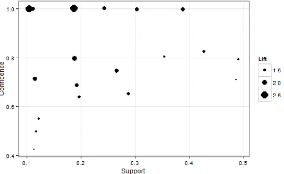
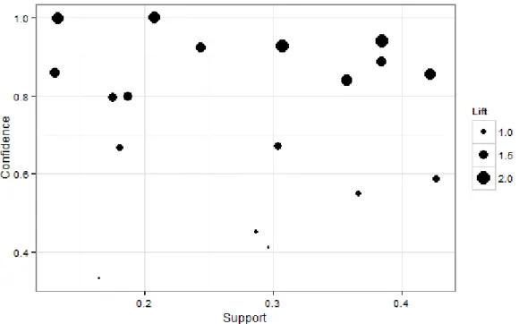
Table 9 reports 19 association rules generated by apriori algorithm. In the former section, it was manageable to inspect all association rules generated due to the smaller number of

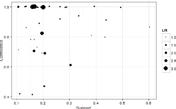
association rules. On the contrary, in this section, the apriori algorithm generates more association rules. In such a case, it is helpful to visualize association rules’ three measures: support, confidence, and lift, so that we can identify strong association rules from the

visualization. Figure 2 depicts the three measures of the 19 association rules. Each point in the plot corresponds to an association rule. A strong association rule, which has high support and confidence, is located in the right upper corner. The large size of a point means the association rule with high lift.

Based on the standard mentioned above, we focus on the 8 points lain in the upper right corner on the plot. First of all, we can identify EDD rule (rule 1, 7, and 12). A released job with sooner due date is always scheduled first (rule 1). Also, the job with either earlier release or longer processing time has a dispatching priority (rule 1, 6, 7, and 9).

(28)

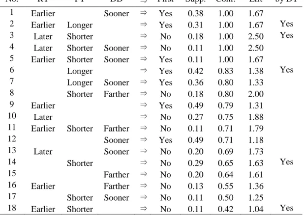
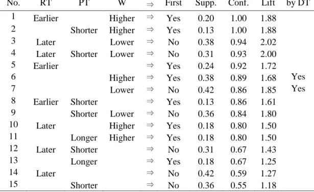
Table 9. Association rules generated from the schedule by EDD rule Rule No. Job 1 RT Job 1 PT Job 1 DD _⇒ Job 1

Found by DT

1 Earlier Sooner ⇒ Yes 0.38 1.00 1.67

2 _Earlier _Longer ⇒ Yes 0.31 1.00 1.67 Yes

3 Later Shorter ⇒ No 0.18 1.00 2.50 Yes

4 _Later _Shorter _Sooner ⇒ No 0.11 1.00 2.50 5 _Earlier _Shorter _Sooner ⇒ Yes 0.11 1.00 1.67

6 Longer ⇒ Yes 0.42 0.83 1.38 Yes

7 _Longer _Sooner ⇒ Yes 0.36 0.80 1.33

8 Shorter Farther ⇒ No 0.18 0.80 2.00

9 _Earlier ⇒ Yes 0.49 0.79 1.31

10 _Later ⇒ No 0.27 0.75 1.88

11 _Earlier _Shorter _Farther ⇒ No 0.11 0.71 1.79

12 _Sooner ⇒ Yes 0.49 0.71 1.18 13 Later Sooner ⇒ No 0.20 0.69 1.73 14 _Shorter ⇒ No 0.29 0.65 1.63 Yes 15 Farther ⇒ No 0.20 0.64 1.61 16 _Earlier _Farther ⇒ No 0.13 0.55 1.36 17 _Shorter _Sooner ⇒ No 0.11 0.50 1.25

(29)

Figure 2. Graphical analysis for identifying strong associations: EDD rule

As before, we select two sets of the core scheduling information from all findings generated. The first set is listed in Table 10. The rules in this table are based on release and processing time. We can also find those rules in the result of the decision tree algorithm. The rule 7, which is respect to processing time of a job, has higher support and confidence than others. Consequently, the C4.5 algorithm selects the “processing time” attribute as a first node. Table 11 reports the second core scheduling information. This set of rules, which corresponds to the actual scheduling rule in this problem, is not revealed by the decision tree algorithm. According to rule 6, for 100% of the instances where a job has earlier release time and sooner due date, the job goes ahead of another.

(30)

Table 10. The first set of core scheduling information: EDD rule Rule No. Job 1 RT Job 1 PT Job 1 DD _⇒ Job 1

Found by DT

2 Earlier Longer ⇒ Yes 0.31 1.00 1.67 Yes

3 _Later _Shorter ⇒ No 0.18 1.00 2.50 Yes

6 Longer ⇒ Yes 0.42 0.83 1.38 Yes

14 _Shorter ⇒ No 0.29 0.65 1.63 Yes

18 _Earlier _Shorter ⇒ No 0.11 0.42 1.04 Yes

Table 11. The second set of core scheduling information: EDD rule Rule No. Job 1 RT Job 1 PT Job 1 DD _⇒ Job 1

Found by DT

1 _Earlier _Sooner ⇒ _Yes _0.38 _1.00 _1.67

5 _Earlier _Shorter _Sooner ⇒ Yes 0.11 1.00 1.67

4.3 Discovering Weighted Shortest Processing Time (WSPT) First Rule

The priority rule that this section follows is Weighted Shortest Processing Time (WSPT) rule, which allocates jobs in decreasing order of 𝑤𝑗/𝑝𝑗. Generally, the WSPT rule is used to

minimize the weighted sum of the completion times, i.e., ∑ 𝑤_𝑗𝐶_𝑗. The dispatching list adopting this principle is shown in Table 12. As before, suppose that it is unknown which rule is adopted, so our task is to discover the WSPT rule using data mining methods. The training data set derived from Table 8 contains a “Job 1 weight” attribute, which examines the job with higher weight.

(31)

Table 12. Job sequence by Weighted Shortest Processing Time (WSPT) first rule Job No. 𝑟_𝑖 𝑝_𝑖 𝑤_𝑖 𝐶_𝑖 6 0 10 7 10 5 9 7 6 17 8 8 9 6 26 1 20 5 5 31 4 8 4 2 35 3 25 7 3 42 9 10 8 3 50 7 14 14 5 64 10 6 7 2 71 2 30 5 1 76

The dispatching rules discovered by C4.5 decision tree algorithm are as below:

 If weight1 = High then job1 goes first

 If weight1 = Lower then job 2 goes first

 If weight1 = Same then job 1 goes first

Based on the findings above, the weight of jobs decides job sequence. Simply, the job weighted more is assigned ahead of the one weighted less. However, the finding of the decision tree algorithm does not completely indicate WSPT principle; we also need the information on processing time to find the actual rule. Furthermore, when the weight of two jobs is the same, there is no clear rule to break the tie. The rule discovered says that job 1 is scheduled first; however, any jobs can be the job 1 while comparing a pair of two jobs. Therefore, we need more information besides weight. We repeat finding rules, in this time, by association rule mining. Table 13 lists association rules generated by apriori algorithm, and Figure 4 visualizes the three measures of corresponding rules. From this graph, we highlight the four points located in the upper right corner as strong associations (rule 1, 2, 3 and 7). First, it can be seen that the job with shorter processing time and higher weight is always scheduled first (rule 1), which means WSPT rule. Another rule identified is simply related to the weight of jobs; for all released jobs,

(32)

the one weighted more is ordered in the front part of the schedule (rule 1 and 3). In addition, there is an association rule, which simply determines job sequence using only weight (rule 7). This rule is the same as the one found by the C4.5 decision tree algorithm.

Table 13. Association rules generated from the schedule by WSPT rule Rule No. Job 1 RT Job 1 PT Job 1 W _⇒ Job 1

Found by DT

1 _Earlier _Higher ⇒ _Yes _0.20 _1.00 _1.88

2 _Shorter _Higher ⇒ Yes 0.13 1.00 1.88

3 _Later _Lower ⇒ No 0.38 0.94 2.02

4 Later Shorter Lower ⇒ No 0.31 0.93 2.00

5 _Earlier ⇒ Yes 0.24 0.92 1.72

6 _Higher ⇒ Yes 0.38 0.89 1.68 Yes

7 _Lower ⇒ No 0.42 0.86 1.85 Yes

8 _Earlier _Shorter ⇒ Yes 0.13 0.86 1.61

9 _Shorter _Lower ⇒ No 0.36 0.84 1.80

10 _Later _Higher ⇒ Yes 0.18 0.80 1.50

11 Longer Higher ⇒ Yes 0.18 0.80 1.50

12 _Later _Shorter ⇒ No 0.31 0.67 1.43

13 _Longer ⇒ Yes 0.18 0.67 1.25

14 _Later ⇒ No 0.42 0.59 1.27

(33)

Figure 3. Graphical analysis for identifying strong associations: WSPT rule

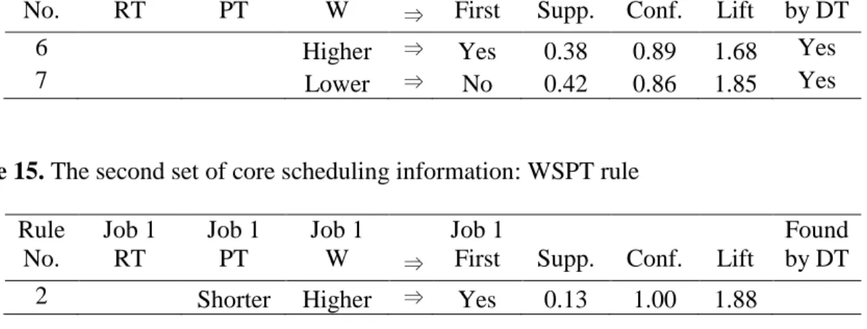
As before, we select two sets of the significant scheduling rules from all the association rules obtained. Table 14 reports the first set. The weight-based rule has dominantly higher

support and confidence than other findings. For example, rule 7 says that a job with lower weight is not scheduled first. This rule occurs in 42% of all instances in the training data. Furthermore, for 86% of cases where a job has lower weight, the job goes later than another. Due to the dominance of this rule, the decision tree algorithm constructs the classification model based on the “weight” attribute. The second set indicating WSPT principle is reported in Table 15. The WSPT is applied with certainty of 100% in this schedule. According to the support of the rule, for 100% of the instances where a job has shorter processing time and higher weight, the job is scheduled first.

(34)

Table 14. The first set of core scheduling information: WSPT rule Rule No. Job 1 RT Job 1 PT Job 1 W _⇒ Job 1

Found by DT

6 Higher ⇒ Yes 0.38 0.89 1.68 Yes

7 _Lower ⇒ No 0.42 0.86 1.85 Yes

Table 15. The second set of core scheduling information: WSPT rule Rule No. Job 1 RT Job 1 PT Job 1 W _⇒ Job 1

Found by DT

4.4 Discovering Weighted Earliest Due Date (WEDD) First Rule

As mentioned in chapter 3, when we want to minimize the maximum lateness, EDD rule is used as a solution. In this section, each job has weight, so the maximum lateness of weighted job is minimized. In other words, Weighted Earliest Due Date (WEDD) first rule places jobs in decreasing order of 𝑤_𝑗/𝑑_𝑗. Table 16 reports the dispatching list following the WEDD principle. As before, we assume that it is unknown which dispatching rule is actually used for this example. Thus, the aim of this section is to find the scheduling rule related to the weight and due date of a job.

(35)

Table 16. Job sequence by Weighted Earliest Due Date (WEDD) first rule Job No. 𝑟_𝑖 𝑝_𝑖 𝑑_𝑖 𝑤_𝑖 𝐶_𝑖 6 0 5 15 7 5 1 4 6 31 2 11 4 6 4 6 3 15 9 11 8 44 5 23 2 18 9 45 5 32 7 24 10 18 5 42 3 34 8 19 7 50 5 36 7 19 3 57 8 23 12 39 3 69 10 10 14 43 1 83

The C4.5 decision tree algorithm discovers following patterns:

 If release time1 = Earlier, then job 1 goes first

 If release time1 = Later, and processing time2 ≤ 10, then job 2 goes first

 If release time1 = Later, and processing time2 > 10, then job 1 goes first

The above decision patterns sequence jobs by release and processing times. First-released job is dispatched earlier. If the released time of a job is later than another, the priority rule depends on the processing time of another job. During the decision tree learning, we fail to find the

scheduling principle in terms of due date and weight. Therefore, association rule mining method analyzes the scheduling data for discovering the hidden rule.

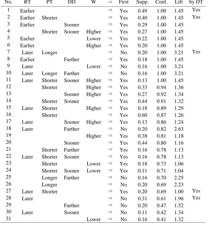
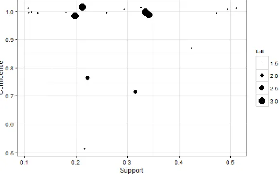
Table 17 reports association rules generated by apriori algorithm. The significance of corresponding rule is graphically analyzed in Figure 4, with the rule’s support, confidence, and lift. From this graph, we select five points where the confidence is 100% and the support is over 25%, at the same time (rule 1, 2, 3 and 4). Also, there is a point, which has a significantly high support, so this point is considered as an important rule (rule 16). Accordingly, total six points are considered as strong associations. The most notable pattern from the six rules selected is earlier-released time first rule (rule 1, 2, and 3). The second notable observation is SPT rule (rule

(36)

2, 4, and 16). In addition, we can identify the rule based on due date and weight (rule 4); the job with sooner due date and higher weight goes ahead of another, which corresponds to WSPT principle.

(37)

Table 17. Association rules generated from the schedule by WEDD rule Rule No. Job 1 RT Job 1 PT Job 1 DD Job 1 W ⇒ Job 1

Found by DT

1 _Earlier ⇒ _Yes _0.49 _1.00 _1.45 Yes

2 _Earlier _Shorter ⇒ Yes 0.40 1.00 1.45 Yes

3 _Earlier _Sooner ⇒ Yes 0.29 1.00 1.45

4 _Shorter _Sooner _Higher ⇒ Yes 0.27 1.00 1.45

5 _Earlier _Lower ⇒ Yes 0.22 1.00 1.45

6 Earlier Higher ⇒ Yes 0.20 1.00 1.45

7 _Later _Longer ⇒ No 0.20 1.00 3.21 Yes

8 Earlier Farther ⇒ Yes 0.18 1.00 1.45

9 _Later _Lower ⇒ No 0.16 1.00 3.21

10 _Later _Longer _Farther ⇒ No 0.16 1.00 3.21

11 _Later _Shorter _Sooner _Higher ⇒ Yes 0.13 1.00 1.45

13 Sooner Higher ⇒ Yes 0.27 0.92 1.34

14 _Shorter _Sooner ⇒ Yes 0.44 0.91 1.32

15 _Later _Shorter _Higher ⇒ Yes 0.18 0.89 1.29

16 _Shorter ⇒ Yes 0.60 0.87 1.26

17 _Later _Sooner _Higher ⇒ Yes 0.13 0.86 1.24

18 Later Farther ⇒ No 0.20 0.82 2.63

19 _Higher ⇒ Yes 0.38 0.81 1.18

20 Sooner ⇒ Yes 0.44 0.80 1.16

21 _Shorter _Farther ⇒ Yes 0.16 0.78 1.13

22 _Later _Shorter _Sooner ⇒ Yes 0.16 0.78 1.13

23 Shorter Lower ⇒ Yes 0.18 0.73 1.06

24 _Shorter _Sooner _Lower ⇒ Yes 0.11 0.71 1.04

25 Longer Farther ⇒ No 0.16 0.70 2.25

26 _Longer ⇒ No 0.20 0.69 2.23

27 _Later _Shorter ⇒ Yes 0.20 0.69 1.00 Yes

28 _Later ⇒ No 0.31 0.61 1.96 Yes

29 _Farther ⇒ No 0.20 0.47 1.52

30 Later Sooner ⇒ No 0.11 0.42 1.34

(38)

Figure 4. Graphical analysis for identifying strong associations: WEDD rule

Two sets of the important scheduling information are extracted from all the association rules obtained. Table 18 reports the first set, where rules are based on release and processing times. Release and processing times of jobs are main factors in this scheduling problem, so the decision tree algorithm selects those as nodes. Table 19 reports the actual scheduling rules. The

information on due date and weight is not found by the decision tree algorithm.

Table 18. The first set of core scheduling information: WEDD rule Rule No. Job 1 RT Job 1 PT Job 1 DD Job 1 W ⇒ Job 1

Found by DT

1 _Earlier ⇒ _Yes _0.49 _1.00 _1.45 Yes

2 Earlier Shorter ⇒ Yes 0.40 1.00 1.45 Yes

7 _Later _Longer ⇒ No 0.20 1.00 3.21 Yes

27 _Later _Shorter ⇒ Yes 0.20 0.69 1.00 Yes

(39)

Table 19. The second set of core scheduling information: WEDD rule Rule No. Job 1 RT Job 1 PT Job 1 DD Job 1 W ⇒ Job 1

Found by DT

3 _Earlier _Sooner ⇒ Yes 0.29 1.00 1.45

4 Shorter Sooner Higher ⇒ Yes 0.27 1.00 1.45

6 _Earlier _Higher ⇒ Yes 0.20 1.00 1.45

(40)

CHAPTER 5

JOB SHOP SCHEDULING APPLICATION

Our framework based on association rule mining approach has so far devoted to the analysis of single machine scheduling problem. Now another important issue for this framework is the applicability to other ranges of schedule data; the approach should be able to analyze other scheduling problems. For example, we question whether our idea can also be applied to the problem with multiple machines, such as job shop or flow shop systems, which is different from single machine problem. The schedule of job shop or flow shop systems corresponds to the dispatching list of each individual machine; multiple machines’ schedule could be divided into a single machine’s job sequence. Ultimately, the analysis of other scheduling problems can be considered as repeating learning from single machine schedule. Thus, it is possible for our approach to be generally used for a wide range of scheduling problem. This chapter will show that the hidden insight in job shop scheduling problem can be discovered by using our approach, as previous case of single machine scheduling problem.

Job shop scheduling problem consists of n jobs and m machines, which is defined as an n

x m problem. Each of n jobs is processed on a set of m machines in a given order. During operations, each machine can process at most one job at a time. Table 20 shows a well-known 6 x 6 job shop scheduling problem [19]. It can be seen that the table includes a pair of values where the left and right number indicate corresponding machine and processing time,

respectively. For example, job 1 has to be processed first on machine 3 for 1-unit time, then on machine 1 for 3-unit time, and so on.

(41)

Table 20. A 6 x 6 job shop scheduling example Operations sequence 1 2 3 4 5 6 Job 1 3, 1 1, 3 2, 6 4, 7 6, 3 5, 6 Job 2 2, 8 3, 5 5, 10 6, 10 1, 10 4, 4 Job 3 3, 5 4, 4 6, 8 1, 9 2, 1 5,7 Job 4 2, 5 1, 5 3, 5 4, 3 5, 8 6, 9 Job 5 3, 9 2, 3 5, 5 6, 4 1, 3 4, 1 Job 6 2, 3 4, 3 6, 9 1, 10 5, 4 3, 1

In general, the objective for job shop scheduling problem is to minimize makespan. The minimum makespan for the example in Table 13 is known to be 55. We cite one of the optimal solutions with 55 makespan from another research [20]. This solution is described as the following dispatching list:

 Machine 1: Job 1 – Job 4 – Job 3 – Job 6 – Job 2 – Job 5

Now the aim of this section is to apply learning method on above dispatching list in order to find scheduling rules. The framework for using learning method is the same as previous chapter. First we transform the dispatching list into a training set. Table 21 refers to the training set derived from the dispatching list on machine 1. In this data set, there is a new attribute, nm

which cannot be seen in the training set of single machine schedule. This attribute describes the number of machines that one job has to visit before arriving at current machine. For example, job 2 must visit or be processed on four machines, 2, 3, 4 and 6 before processing on current

(42)

machine 1; job 2 has the value, 4 for nm attribute. After training sets for each machine are

generated, decision tree and association rule mining learning examine what scheduling principles were used for the training set. Similar to this work, dispatching rules for job shop scheduling problem were found by decision tree algorithm [21].

Table 21. The training set derived from the schedule of machine 1 Job 1 𝑟1 𝑝1 𝑛𝑚1 Job 2 𝑟2 𝑝2 𝑛𝑚2 Job 1

RT Job 1 PT Job 1 NM Job 1 First

1 1 3 1 2 33 10 4 Earlier Shorter Less Yes

1 1 3 1 4 5 5 1 Earlier Shorter Same Yes

. . . .

5 21 3 4 6 15 10 3 Later Shorter More No

5.1 Discovering Scheduling Rules for Machine 1

We first analyze the scheduling data on machine 1 to discover dispatching rules. The decision tree algorithm generates the following rules:

 If number of machines1 = Less or Same then job 1 goes first

 If number of machines1 = More then job 2 goes first

According to above rules, on machine 1 jobs are allocated by the value of “number of machines” attribute. If a job is supposed to be processed on machine 1 in early operations sequence, the job will be dispatched first. In job shop system, the route of each job is pre-specified, so the “number of machines” attribute would play an important role in scheduling. Consequently, the decision tree algorithm discovers the rule based on the “number of machines” attribute. In the next step, we inspect the result of association rule mining method.

(43)

The support, confidence, and lift of association rules are visualized in Figure 6, and Table 22 reports corresponding association rules. The most notable pattern is Earliest Release Date (ERD) first rule (rule 1, 4, and 15). Above all, the rule 1, which indicates the ERD principle, has the highest support in the table. Also, it is observed that Shortest Processing Time (SPT) first rule is used (rule 5 and 17). In addition, the rule based on “number of machines” attribute is reaffirmed (rule 2 and 3), which is discovered by the decision tree algorithm.

Table 22. Association rules generated from the schedule of machine 1 Rule No. Job 1 R.T. Job 1 P.T. Job 1 N.M. ⇒ Job 1

Found by tree

1 _Earlier ⇒ _Yes _0.53 _1.00 _1.50

2 Less ⇒ Yes 0.47 1.00 1.50 Yes

3 _More ⇒ No 0.33 1.00 3.00 Yes

5 Later More ⇒ No 0.33 1.00 3.00

6 Shorter Less ⇒ Yes 0.27 1.00 1.50

7 Same ⇒ Yes 0.20 1.00 1.50 Yes

8 Longer More ⇒ No 0.20 1.00 3.00

9 Earlier Longer ⇒ Yes 0.13 1.00 1.50

10 Later Same ⇒ Yes 0.13 1.00 1.50

11 Shorter Same ⇒ Yes 0.13 1.00 1.50

12 Longer Less ⇒ Yes 0.13 1.00 1.50

13 Shorter ⇒ Yes 0.40 0.86 1.29

14 Later Longer ⇒ No 0.20 0.75 2.25

15 Later ⇒ No 0.33 0.71 2.14

(44)

Figure 5. Graphical analysis for identifying strong associations: machine 1

Table 23 reports the first set of the core scheduling information. The rule with respect to

“number of machines” attribute can be checked in the stage of the decision tree induction. On the other hand, Table 24 lists the additional information other than “number of machines” attribute. In this table, we can check earlier release time first and shorter processing time first rules.

Table 23. The first set of the core scheduling information: Machine 1 Rule No. Job 1 R.T. Job 1 P.T. Job 1 N.M. ⇒ Job 1

Found by tree

2 _Less ⇒ Yes 0.47 1.00 1.50 Yes

3 More ⇒ No 0.33 1.00 3.00 Yes

(45)

Table 24. The second set of the core scheduling information: Machine 1 Rule No. Job 1 R.T. Job 1 P.T. Job 1 N.M. ⇒ Job 1

Found by tree

1 _Earlier ⇒ Yes 0.53 1.00 1.50

This section examines the dispatching rules used on machine 2. The decision tree algorithm analyzes the data derived from the dispatching list of machine 2. As a result, the algorithm generates the following rules:

 If release time1 = Same or Earlier then job 1 goes first

 If release time1 = Later then job 2 goes first

As it can be seen above, the schedule on machine 2 depends on jobs’ release time; if a job is released earlier, the job goes first. In the result of the decision tree, the information regarding “processing time” or “number of machines” attribute is unavailable. In the next learning stage, we use association rule mining method.

Figure 5 graphically shows the significance of the association rules discovered by the apriori algorithm. Corresponding rules are reported in Table 25. The first pattern identified is ERD principle (rule 1, 2, 3 and 4). Similar to the principle on “release time” attribute, the rule based on “number of machines” attribute is detected (rule 2 and 14). In addition, Longest Processing Time (LPT) first rule is applied in the schedule on machine 2 (rule 4 and 15).

(46)

Found by tree

1 _Later ⇒ No 0.47 1.00 2.14 Yes

2 _Later _More ⇒ No 0.47 1.00 2.14

3 _Earlier ⇒ Yes 0.33 1.00 1.88 Yes

4 _Earlier _Longer ⇒ Yes 0.33 1.00 1.88

5 Shorter ⇒ No 0.27 1.00 2.14

6 Less ⇒ Yes 0.27 1.00 1.88

7 Shorter More ⇒ No 0.27 1.00 2.14

8 Longer Less ⇒ Yes 0.27 1.00 1.88

9 Same ⇒ Yes 0.20 1.00 1.88 Yes

10 Same ⇒ Yes 0.20 1.00 1.88

11 Same Longer ⇒ Yes 0.20 1.00 1.88

12 Longer Same ⇒ Yes 0.20 1.00 1.88

13 Later Longer ⇒ No 0.13 1.00 2.14

14 More ⇒ No 0.47 0.88 1.88

15 Longer ⇒ Yes 0.53 0.80 1.50

16 Longer More ⇒ No 0.13 0.67 1.43

(47)

The decision tree algorithm selects “release time” attribute as the most important information. This result is reaffirmed by the apriori algorithm. Table 26 extracts the most important information on the “release time” attribute again. Table 27 summarizes another

important information on the “processing time” attribute. A job with longer processing time goes first. On the contrary, a job with shorter processing time is not scheduled first. This information is not identified during the decision tree induction.

Table 26. The first set of core scheduling information: Machine 2 Rule No. Job 1 R.T. Job 1 P.T. Job 1 N.M. ⇒ Job 1

Found by tree

1 _Later ⇒ _No _0.47 _1.00 _2.14 Yes

3 Earlier ⇒ Yes 0.33 1.00 1.88 Yes

9 Same ⇒ Yes 0.20 1.00 1.88 Yes

Table 27. The second set of core scheduling information: Machine 2 Rule No. Job 1 R.T. Job 1 P.T. Job 1 N.M. ⇒ Job 1

Found by tree

5 Shorter ⇒ No 0.27 1.00 2.14

6 Less ⇒ Yes 0.27 1.00 1.88

7 Shorter More ⇒ No 0.27 1.00 2.14

8 Longer Less ⇒ Yes 0.27 1.00 1.88

10 Same ⇒ Yes 0.20 1.00 1.88

11 Same Longer ⇒ Yes 0.20 1.00 1.88

12 Longer Same ⇒ Yes 0.20 1.00 1.88

In this section, the scheduling data of machine 3 is analyzed for discovering dispatching strategies. First, the C4.5 algorithm reveals the below decision rules:

(48)

 If release time1 = Same or Earlier then job 1 goes first

 If release time1 = Later then job 2 goes first

The above rules is on the basis of release time; it directly indicates ERD rule. Second, the apriori algorithm continues the analysis of the scheduling data on the machine 3.

Figure 7 graphically shows the strength of association rules by the rules’ support,

confidence, and lift. Corresponding rules are listed in Table 28. From the plot and table, it can be seen that two rules have support of 60% (rule 1 and 2). The first rule indicates ERD rule. The second rule is based on “number of machines” attribute; a scheduling priority is given to the job which should visit machine 3 at the beginning. These two rules regarding “release time” and “number of machines” attributes are consistently applied in this machine. The pattern relevant to processing time is not identified.

Found by tree

1 _Earlier ⇒ _Yes _0.60 _1.00 _1.25 Yes

2 Less ⇒ Yes 0.60 1.00 1.25

3 Longer ⇒ Yes 0.27 1.00 1.25

4 Earlier Same ⇒ Yes 0.20 1.00 1.25

5 Same Less ⇒ Yes 0.20 1.00 1.25

8 Later ⇒ No 0.13 0.67 3.33 Yes

9 More ⇒ No 0.13 0.67 3.33

10 Later More ⇒ No 0.13 0.67 3.33

(49)

Figure 7. Graphical analysis for identifying strong associations: machine 3

The first core scheduling information is summarized in Table 29. This rule set corresponds to the earlier release time first rule, which can also be seen in the decision tree algorithm’s finding. Table 30 lists the second core scheduling information. The information on “number of machine” attribute can be identified. However, it is difficult to find the pattern for processing time; according to the rules in this table, the jobs with both longer processing time and shorter processing time go first with confidence of 100%. Processing time does not significantly affect the schedule on this machine.

Table 29. The first set of core scheduling information: Machne 3 Rule No. Job 1 R.T. Job 1 P.T. Job 1 N.M. ⇒ Job 1

Found by tree

1 _Earlier ⇒ _Yes _0.60 _1.00 _1.25 Yes

(50)

Found by tree

2 _Less ⇒ Yes 0.60 1.00 1.25

3 Longer ⇒ Yes 0.27 1.00 1.25

5 Same Less ⇒ Yes 0.20 1.00 1.25

We continue the analysis of the scheduling data on machine 4. The first learning method, C4.5 algorithm builds the following scheduling model:

 If number of machine1 = Same or Less then job 1 goes first

 If number of machine1 = More then job 2 goes first

The above model provides dispatching rules depending on “number of machine” attribute; the job with the smaller value of “number of machines” has a scheduling priority. Next, we discuss the result of association rule mining method.

Figure 8 depicts the significance of the association rules created by the apriori algorithm. Corresponding rules are listed in Table 31. The most notable pattern is the same as the output of the decision tree algorithm; the value of “number of machines” attribute determines the job order (rule 1, 2, 3, 4, and 5). We can also identify ERD (rule 2 and 4), and LPT principles (rule 5, 12 and 17). The LPT principle is applied for all released jobs on machine 4.

(51)

Found by tree

1 _More ⇒ No 0.47 1.00 1.88 Yes

2 _Later _More ⇒ No 0.47 1.00 1.88

3 _Less ⇒ Yes 0.33 1.00 2.14 Yes

4 _Earlier _Less ⇒ Yes 0.33 1.00 2.14

5 Longer Less ⇒ Yes 0.33 1.00 2.14

6 Longer More ⇒ No 0.27 1.00 1.88

7 Same ⇒ No 0.13 1.00 1.88

8 Later Same ⇒ Yes 0.13 1.00 2.14

9 Later Same ⇒ No 0.13 1.00 1.88

10 Later Longer Same ⇒ Yes 0.13 1.00 2.14

11 Earlier ⇒ Yes 0.33 0.83 1.79

13 Later ⇒ No 0.47 0.78 1.46

14 Later Longer ⇒ No 0.27 0.67 1.25

15 Same ⇒ Yes 0.13 0.67 1.43 Yes

16 Longer Same ⇒ Yes 0.13 0.67 1.43

17 Longer ⇒ Yes 0.47 0.58 1.25

(52)

Table 32 reports the first set of core scheduling information, which is according to “number of machines” attribute. This information can be seen in the result of the decision tree algorithm. Table 33 lists another set of scheduling information. In this set of rules, new information on release and processing times can be obtained.

Table 32. The first set of core scheduling information: Machine 4 Rule No. Job 1 R.T. Job 1 P.T. Job 1 N.M. ⇒ Job 1

Found by tree

1 _More ⇒ No 0.47 1.00 1.88 Yes

3 _Less ⇒ Yes 0.33 1.00 2.14 Yes

16 Same ⇒ Yes 0.13 0.67 1.43 Yes

Found by tree

2 Later More ⇒ No 0.47 1.00 1.88

4 _Earlier _Less ⇒ Yes 0.33 1.00 2.14

5 _Longer _Less ⇒ Yes 0.33 1.00 2.14

In this section, we aim at mining the dispatching principles for machine 5. In the first learning stage, the findings of the C4.5 algorithm are as below:

 If processing time1 ≤ 6 then job 2 goes first

 If processing time1 > 6 and number of machines2 ≤ 2 then job 2 goes first

(53)

According to the findings above, jobs are ordered based on specific values of the “processing time” and “number of machines” attributes. Next, association rule mining algorithm analyzes the scheduling data of machine 5.

Figure 9 visually shows the quality of the association rules. As it can be seen, there are a few points on the upper right corner on this plot; it is difficult to see the rules with high support and confidence. Corresponding rules are summarized in Table 34. The association rules in this table consistently report that a scheduling priority goes to the job with either earlier release time or the smaller value of “number of machines” attribute, and vice versa.

Found by tree

1 _Longer _Same ⇒ _Yes _0.13 _1.00 _2.14 Yes

2 Longer More ⇒ No 0.27 0.80 1.50 Yes

3 More ⇒ No 0.40 0.75 1.41

4 _Shorter ⇒ No 0.20 0.75 1.41 Yes

5 Less ⇒ Yes 0.20 0.75 1.61

6 Earlier Less ⇒ Yes 0.20 0.75 1.61

7 Longer Less ⇒ Yes 0.20 0.75 1.61 Yes

8 Later Longer More ⇒ No 0.20 0.75 1.41

9 Earlier Longer Less ⇒ Yes 0.20 0.75 1.61

10 Later More ⇒ No 0.33 0.71 1.34

12 Same ⇒ Yes 0.13 0.67 1.43