Simultaneous Bayesian analysis of contingency tables in genetic association studies

Weierstraß-Institut

für Angewandte Analysis und Stochastik

Leibniz-Institut im Forschungsverbund Berlin e. V.

Preprint

ISSN 2198-5855

Simultaneous Bayesian analysis of contingency tables in

genetic association studies

Thorsten Dickhaus

submitted: August 15, 2014 Weierstrass Institute Mohrenstr. 39 10117 Berlin E-Mail: [email protected] No. 1995 Berlin 2014

2010Mathematics Subject Classification. 62J15, 62C10.

Key words and phrases. Bayes factor, decision theoretic multiple test procedure, Dirichlet mixture, effective number of tests, simultaneous statistical inference.

This work makes use of data generated by the Wellcome Trust Case Control Consortium. A full list of the investiga-tors who contributed to the generation of the data is available fromhttp://www.wtccc.org.uk. Funding for the Wellcome Trust Case Control Consortium project was provided by the Wellcome Trust under award 076113.

Edited by

Weierstraß-Institut für Angewandte Analysis und Stochastik (WIAS) Leibniz-Institut im Forschungsverbund Berlin e. V.

Mohrenstraße 39 10117 Berlin Germany

Fax: +49 30 20372-303

E-Mail:

[email protected]

Abstract

Genetic association studies lead to simultaneous categorical data analysis. The sample for every genetic locus consists of a contingency table containing the numbers of observed genotype-phenotype combinations. Under case-control design, the row counts of every ta-ble are identical and fixed, while column counts are random. The aim of the statistical analysis is to test independence of the phenotype and the genotype at every locus. We present an objective Bayesian methodology for these association tests, utilizing the Bayes factor proposed by Good (1976) and Crook and Good (1980). It relies on the conjugacy of Dirichlet and multinomial distributions, where the hyperprior for the Dirichlet parameter is log-Cauchy. Being based on the likelihood principle, the Bayesian tests avoid looping over all tables with given marginals. Hence, their computational burden does not increase with the sample size, in contrast to frequentist exact tests. Making use of data generated by The Wellcome Trust Case Control Consortium (2007), we illustrate that the ordering of the Bayes factors shows a good agreement with that of frequentistp-values. Furthermore, we deal with specifying prior probabilities for the validity of the null hypotheses, by taking link-age disequilibrium structure into account and exploiting the concept of effective numbers of tests. Application of a Bayesian decision theoretic multiple test procedure to The Well-come Trust Case Control Consortium (2007) data illustrates the proposed methodology. Finally, we discuss two methods for reconciling frequentist and Bayesian approaches to the multiple association test problem for contingency tables in genetic association studies.

1

Introduction

Testing for association between two categorical variates by means of contingency table data is a classical problem in statistics which can at least be traced back to Pearson (1900) and Fisher (1922). For a comprehensive account of frequentist tests for this problem we defer the reader to Agresti (2002). Bayesian methodology for categorical data analysis is nicely summarized by Agresti and Hitchcock (2005); see also Gómez-Villegas and González-Pérez (2010) for later developments.

In this work, we are considered with applications of Bayesian inference for contingency tables to the field of genetic association studies with case-control setup. From the statistical point of view, such studies lead to the problem of simultaneous categorical data analysis, meaning that many contingency tables have to be analyzed simultaneously. Assuming a set of

m >

1

bi-allelic genetic markers with exactly two possible values

A

j,1 and

A

j,2(say) for

1

≤

j

≤

m, the

data for genetic locus

j

can in such type of study be summarized as in Table 1. Typically, single nucleotide polymorphisms (SNPs) are used as markers, such that

A

j,1

, A

j,2

∈ {

A, C, G, T

}

encode base pairs. However, our methodology is not restricted to SNP studies, but can also be applied to more complex markers such as copy number variations (CNVs) of sections of the

deoxyribonucleic acid (DNA), as long as the CNVs have the same binary status as SNPs as considered by McCarroll et al. (2008), for example.

Table 1: Schematic representation of data for an association test problem at genetic locus

j,

where the two possible alleles are denoted by

A

j,1 and

A

j,2.

Genotype

A

j,1

A

j,1

A

j,1

A

j,2

A

j,2

A

j,2

P

Phenotype

1

x

(j)₁₁

x

(j)₁₂

x

(j)₁₃

n

1.

Phenotype

0

x

(j)₂₁

x

(j)₂₂

x

(j)₂₃

n

2.

Absolute count

n

.1(j)

n

.2(j)

n

.3(j)

N

The numbers

n

1.of cases (phenotype

1) and

n

2.of controls (phenotype

0) do not depend on

j

and are fixed by experimental design. The aim of the statistical analysis is to test the family of hypotheses

H

= (H

j

: 1

≤

j

≤

m), where the

j-th null hypothesis

H

j states that the

genotype at locus

j

is stochastically independent of the (binary) phenotype of interest. The corresponding (two-sided) alternatives are denoted by

K

j,

1

≤

j

≤

m.

In the remainder of this work, for notational convenience, we will write

x

=

x

11

x

12

x

13

x

21

x

22

x

23

instead of

x

(j)

=

x

(j) 11

x

(j) 12

x

(j) 13

x

(j)₂₁

x

(j)₂₂

x

(j)₂₃

!

for the data sample if only one specific locus is con-cerned. Similarly, we will in such cases drop the subscript

j

in

H

and

K

and the superscript

j

in

n

.1,

n

.2, and

n

.3for ease of presentation, although column counts depend on

j. The conditional

probability of observing

x

under the null hypothesis of no association, given all marginal counts

n

= (n

1.

, n

2.

, n

.1

, n

.2

, n

.3

)

>, will be denoted by

f

(

x

|

n

)

and is (in a compact, self-explaining

notation) given by

f(

x

|

n

) =

Q

n∈_n

n!

N

!

Q

x∈x

x!

.

(1)

Frequentist exact tests enumerate all tables

x

˜

with marginals equal to

n

according to some real-valued test statistic

T

:

X →

R

_{in order to compute a}

_{p-value, cf. Langaas and Bakke}

(2013) and references therein. Assuming that

T

tends to smaller values under the alternative, the non-asymptotic

p-value based on

T

and conditional to

n

is given by

p

T

(

x

) =

X

˜

x:T(˜x)≤T(x)

f(˜

x

|

n

) =

P

_(T

₍

_X

₎

_≤

_T

₍

_x

₎

_|

_H,

_n

₎

_.

₍₂₎

The remaining part of the paper is structured as follows. In Section 2, we revisit and work up the computation of Bayes factors for testing association in a single contingency table according to Good (1976) and Crook and Good (1980). Section 3 is devoted to the numerical computa-tion of these Bayes factors. In Seccomputa-tion 4, we apply the proposed Bayes factors to real genetic association data generated by The Wellcome Trust Case Control Consortium (2007). Section 5 completes the probability model by discussing prior probabilities for the null hypotheses

H

j,

1

≤

j

≤

m, and we apply a Bayesian decision theoretic multiple comparison procedure to the

the Bayesian approach to the multiple association test problem. These methods may be consid-ered as alternatives to the asymptotic (

N

→ ∞

) approach by Wakefield (2009). We conclude with a discussion in Section 7.

2

Statistical methodology

Motivated by the conjugacy of Dirichlet and multinomial distributions, Good (1976) and Crook and Good (1980) proposed objective Bayesian inference for one single contigency table in the following manner.

Let

X

= (X

ν

)

1≤ν≤tdenote a random vector with

t

integer elements which takes values in the

discrete set

X

=

{

(x

1

, . . . , x

t

)

>

∈

N

0t

: 0

≤

x

ν

≤

N

for all

1

≤

ν

≤

t,

t

X

ν=1

x

ν

=

N

}

.

Furthermore, consider a vector

p

= (p

1

, . . . , p

t

)

>which is Dirichlet distributed on the (closed)

unit simplex in

[0,

1]

t_{with parameter vector}

_a

_{= (a}

1

, . . . , a

t

)

>, such that the conditional

dis-tribution of

X

given

p

is multinomial with

t

categories, total sample size

N

and vector

p

of cell probabilities,

M

(t, N,

p

)

for short. Assuming

a

1

=

a

2

=

. . .

=

a

t

=

a, the unconditional

distribution of

X

is the (symmetric) Dirichlet-multinomial distribution with flattening parameter

a,

which we will denote by DMultinomial(t, N, a). Its probability mass function is given by

DMultinomial

((x

ν

)

|

t, N, a) =

N

(x

ν

)

Γ(ta)

{

Γ(a)

}

t

Q

t ν=1

Γ(x

ν

+

a)

Γ(N

+

ta)

,

(x

ν

)

∈ X

;

(3) see, for instance, Section 6.1.2 of Ng et al. (2011). In (3) and throughout the remainder, we use the abbreviated notation

(x

ν

)

for

(x

1

, . . . , x

t

)

>. In the derivations of Good (1976) and Crook

and Good (1980), the function

Φ, given by

Φ((x

ν

), t, t

0

) =

Z

∞ 0 DMultinomial

((x

ν

)

|

t, N, a)

φ

a

t

0

da

t

0

,

(4)

plays a crucial role. In (4) and throughout the remainder,

φ

denotes the Lebesgue density of the log-Cauchy distribution with location

0

and scale

π, given by

φ(u) =

1

u[π

2

_{+ ln}

2

_(u)]

,

u >

0.

(5)

As argued by Good (1976), p. 1163, the log-Cauchy(0, π)hyperprior for the flattening parameter is a proper proxy for the improper Jeffrey-Haldane density

u

7→

u

−1_{, and therefore particularly}

suitable for objective Bayesian contingency table analysis. Henceforth, the symmetric Dirichlet mixture prior with

t

categories and log-Cauchy(0, π)hyperprior with scaling parameter

t

0 _for

_a

is denoted by

D

∗

_{(t, t}

0

_).

Returning to the case-control studies introduced in Section 1, recall that the row sums

n

1.and

one specific locus and under the corresponding null hypothesis, the only unknown model pa-rameters are the multinomial probabilities

p

.1,

p

.2, and

p

.3 for the column counts. Good (1976)

proposed the

D

∗

_(3,

₁₎

_{prior for}

_(p

.1

, p

.2

, p

.3

)

> under the null, leading to a prior probability

of

Φ((n

.k

),

3,

1)

for the column counts, where

1

≤

k

≤

3. Based on this, the probability

of observing

x

under the null is equal to

P

₍

_x

_|

_n

_1.

_{, n}

_2.

_{, H}

_{) = Φ((n}

_.k

_),

_3,

₁₎

_×

_f

₍

_x

_|

_n

₎

. Analo-gously, under the alternative, the

D

∗

_(6,

₁₎

_{prior is assumed for the six unknown cell probabilities}

(p

ik

: 1

≤

i

≤

2,

1

≤

k

≤

3), such that

Φ(

x

,

6,

1)

gives the unconditional probability of

ob-serving

x

under the alternative. As the Dirichlet prior

D

∗

(6,

1)

necessarily implies the

D

∗

(2,

3)

prior for the row counts, we obtain that

P

₍

_x

_|

_n

_1.

_{, n}

_2.

_{, K) = Φ(}

_x

_,

_6,

_1)/Φ((n

_1.

_{, n}

_2.

₎

>

_,

_2,

_3).

Altogether, this entails the Bayes factor

F

2

=

P

₍

_x

_|

_n

_1.

_{, n}

_2.

_{, H}

₎

P

₍

x

|

n

1.

, n

2.

, K)

=

Φ (n

1.

, n

2.

)

>

_,

_2,

₃

Φ((n

.k

),

3,

1)f(

x

|

n

)

Φ(

x

,

6,

1)

for testing

H

versus

K, where the subscript

2

indicates that only the column counts (second dimension of the table) are random.

Remark 1.

(i) Actually, Good (1976) and Crook and Good (1980) developed the methodology described

in this section for general

(R

×

C)

-tables. For our purposes, however, only the special

case of

R

= 2

and

C

= 3

is relevant.

(ii) Crook and Good (1980) also discussed further choices for the scale parameter, say

s

,

of the log-Cauchy density in(5). Exemplary computations (not shown here) however

in-dicated that the Bayes factor

F

2 is not very sensitive with respect to

s

, at least if

F

2 is

small. Therefore, we made use of the original recommendation by Good (1976) and took

s

=

π

.

3

Computational details

Although the computation of

F

2 is rather straightforward, some caution is required in actual

implementation. As far as software is concerned, we implemented all routines described in this section in

MATLAB. This choice is mainly motivated by the fact that

MATLAB

provides the fully vectorized function

gammaln

for evaluating the logarithmic Gamma function, which plays a pivotal role in computing

F

2. Based on this function, the computation of

f

(

x

|

n

)

has already

3.1

Computation of DMultinomial

((

x

ν

)

|

t, N, a

)

Taking logarithms in (3), we obtain that

ln (DMultinomial

((x

ν

)

|

t, N, a)) =

"

ln(Γ(N

+ 1))

−

t

X

ν=1

ln(Γ((x

ν

+ 1))

#

+

(6)

ln

Γ(ta)

{

Γ(a)

}

t

Q

t ν=1

Γ(x

ν

+

a)

Γ(N

+

ta)

.

(7)

The right-hand side of (6) is directly evaluatable with the

gammaln

function, while the sum-mand displayed in (7) is efficiently implemented in the contributed

MATLAB

program

polya_logProb.m

from the

Fastfit

toolbox by Thomas Minka.

As one additional pitfall, notice that the log-Cauchy distribution can produce extremely large real-izations of the flattening parameter

a, which leads to numerical problems in the

polya_logProb.m

program. On the other hand, we can exploit the well-known fact that the symmetric Dirichlet dis-tribution degenerates for

a

→ ∞

, such that the random vector

p

= (p

1

, . . . , p

t

)

>tends to the

constant vector

p

∗

_{= (t}

−1

_{, . . . , t}

−1

₎

>_{almost surely as}

_a

_{→ ∞}

_{. Consequently, it is possible}

to accurately approximate DMultinomial

(t, N, a)

by

M

(t, N,

p

∗

)

whenever

a

exceeds some threshold

a

upper. In our implementation, we chose

a

upper

= 10

6. This choice was motivated

by some preliminary example computations which indicated that, within the range of numerical double precision, the difference between DMultinomial(t, N, a)and

M

(t, N,

p

∗

)

is negligible for

a >

10

6_.

3.2

Computation of

Φ((

x

ν

)

, t, t

0

)

Recall that

Φ((x

ν

), t, t

0

) =

Z

∞ 0 DMultinomial

((x

ν

)

|

t, N, a)

φ

a

t

0

da

t

0

=

E

_A∼t0_{log-Cauchy(0,π)}

[DMultinomial

((x

_ν

)

|

t, N, A)]

.

(8)

While the integral representation in (4) appears more convenient for numerical evaluation, it turned out that numerical integration with respect to

φ

is rather challenging. Neither the quadra-ture routines in

MATLAB

nor those in

R

could even verify that

φ

is a probability density. There-fore, we made use of the equivalent representation in (8) and performed Monte Carlo inte-gration. Namely, the theoretical expectation in (8) was replaced by the arithmetic mean of the integrand evaluated at

B

pseudo-random numbers which behave like independent realizations of

A

∼

t

0

log-Cauchy(0, π). In our implementation, we used

B

= 100,000, leading to a small

Monte Carlo standard error.

3.3

Computational complexity

As mentioned in the discussion around (1) and (2), a loop over all possible tables with given marginals

n

cannot be avoided if exact frequentist tests are to be carried out. Clearly, the num-ber of such tables that have to be enumerated increases drastically with the sample size

N

,

see Bakke and Langaas (2012). Unconditional asymptotic tests, typically based on chi-square approximations, are often considered a convenient alternative for large

N

. However, the chi-square approximation can be very poor in extreme tail areas, even if

N

is very large, cf. Langaas and Bakke (2013). Hence, if

m

is large and a strong multiplicity adjustment is necessary (high quantiles of the null distribution of the test statistic are needed), the chi-square approximation is doubtful. Clearly, there are other (asymptotic or non-asymptotic) frequentist test approaches which are under certain assumptions on the expected cell counts more robust than chi-square tests; see, e. g., Lydersen et al. (2009) for a biostatistics tutorial with practical guidelines for choosing a marginal testing strategy in the case of a (2

×

2)-table. However, an automated

application of such guidelines for a large number of contingency tables simultaneously, where parameters like the expected minor allele frequency are prone to change considerably from one genomic position to the other, appears extremely challenging.

In contrast to these problems, the computational complexity of computing

F

2 remains constant

for any

N

. Plainly speaking, the reason is that the parameter space for

(p

ik

: 1

≤

i

≤

2,

1

≤

k

≤

3)

is independent of

N

, while the sample space

X

crucially depends on

N

. Being based on the likelihood principle, Bayesian tests do not have to explore the sample space, but the parameter space. Also, no asymptotic considerations are required. The only costly (non-scalar) operation in our implementation of

F

2is the generation of

B

pseudo-random Cauchy numbers,

see Section 3.2. However, from our experience it is not necessary to choose

B

as a function of

N.

Remark 2. All

MATLAB

worksheets that were used to derive the results presented in this paper are available as supplementary material from the author upon request.

4

Computation of Bayes factors from real data

In this section, we apply the proposed methodology to the Crohn’s disease substudy reported by The Wellcome Trust Case Control Consortium (2007). More precisely, we restricted our attention to

m

= 1,778

pre-screened loci. The pre-screening has been performed by sample-splitting with respect to

N

and applying a false discovery rate-based screening criterion to the first subsample of size

N/2

as described in Section 6.2 of Dickhaus et al. (2012). The computation of

F

₂(j)for

1

≤

j

≤

m

= 1,778

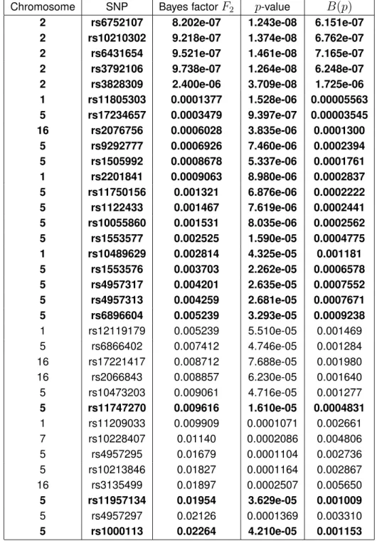
was performed on the second subsample which has not been used for screening. This mimics a two-stage study design which is often chosen in genome-wide association studies.

Table 2 displays the

34

smallest of the

1,778

Bayes factors in increasing order. Bold-face rows indicate SNPs that were declared significantly associated with Crohn’s disease by the multiple test from Section 3.4 of Dickhaus et al. (2012); see Table 3 in their paper. It becomes apparent that the

34

positions with smallest Bayes factors comprise

23

out of the

24

loci with significant associations reported by Dickhaus et al. (2012). A closer investigation of the data corresponding to the only “non-replicated“ SNP, namely rs11816049 with Bayes factor

F

₂(rs11816049)

= 6.85722,

revealed that the significance reported in Table 3 of Dickhaus et al. (2012) for this SNP is actually an artifact of their randomization technique. The contingency table for this locus is given by

x

(rs11816049)

₌

0 1 874

0 0 1468

. Conditional to all five marginal counts, there are only two possible realizations of this table. Therefore, one can randomize the entire table probability of

f(

x

(rs11816049)

_|

_n

_{) = 0.3735, and this has lead to the artifactually small}

_{p-value for rs11816049}

in Table 3 of Dickhaus et al. (2012). The last column of Table 2 compares the frequentist

p-values with Bayes factors quantitatively. Namely, we applied the “p-value calibration“ method

B(p)

by Sellke et al. (2001) to the

p-values from the fourth column. As the authors argue below

their equation (2),

B(p)

provides a lower bound on the Bayes factor. This property is numerically verified by our data.

While Table 2 focusses on the

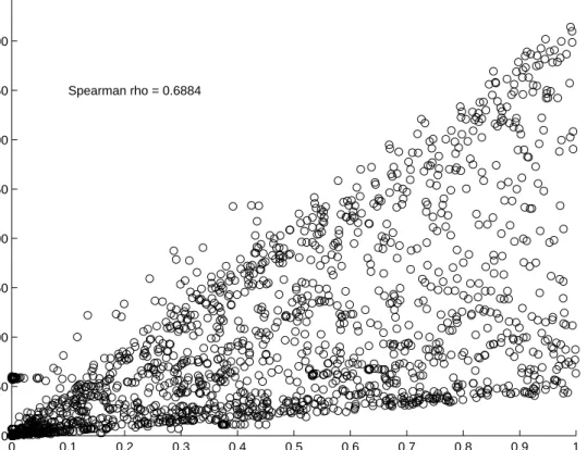
34

smallest Bayes factors, Figure 1 displays a scatter plot of

p-values against Bayes factors for all

m

= 1,778

SNPs under investigation. The high value

of approximately

0.69

for Spearman’s rank correlation coefficient between the two quantities confirms that the good accordance between the orderings of frequentist

p-values and Bayes

factors extends beyond the subset of small Bayes factors.

0 0.1 0.2 0.3 0.4 0.5 0.6 0.7 0.8 0.9 1 0 50 100 150 200 250 300 350 400 450 p-values Bayes Factors Spearman rho = 0.6884

Figure 1: Scatter plot of

p-values against Bayes factors computed from data for

m

= 1,778

pre-screened genomic positions. Data were generated by The Wellcome Trust Case Control Consortium (2007), sub-study for Crohn’s disease.

Table 2: The

34

smallest Bayes factors computed from the data on Crohn’s disease reported by The Wellcome Trust Case Control Consortium (2007). Bold-face rows correspond to significant associations when applying the frequentist multiple test from Section 3.4 of Dickhaus et al. (2012). The last column contains a lower bound on the Bayes factor as a function of the

p-value

from the fourth column; see equation (2) of Sellke et al. (2001).

Chromosome SNP Bayes factor

F

2

p-value

B(p)

2 rs6752107 8.202e-07 1.243e-08 6.151e-07 2 rs10210302 9.218e-07 1.374e-08 6.762e-07 2 rs6431654 9.521e-07 1.461e-08 7.165e-07 2 rs3792106 9.738e-07 1.264e-08 6.248e-07 2 rs3828309 2.400e-06 3.709e-08 1.725e-06 1 rs11805303 0.0001377 1.528e-06 0.00005563 5 rs17234657 0.0003479 9.397e-07 0.00003545 16 rs2076756 0.0006028 3.835e-06 0.0001300 5 rs9292777 0.0006926 7.460e-06 0.0002394 5 rs1505992 0.0008678 5.337e-06 0.0001761 1 rs2201841 0.0009063 8.980e-06 0.0002837 5 rs11750156 0.001321 6.876e-06 0.0002222 5 rs1122433 0.001467 7.619e-06 0.0002441 5 rs10055860 0.001531 8.035e-06 0.0002562 5 rs1553577 0.002525 1.590e-05 0.0004775 1 rs10489629 0.002814 4.325e-05 0.001181 5 rs1553576 0.003703 2.262e-05 0.0006578 5 rs4957317 0.004201 2.635e-05 0.0007552 5 rs4957313 0.004259 2.681e-05 0.0007671 5 rs6896604 0.005239 3.293e-05 0.0009238 1 rs12119179 0.005239 5.510e-05 0.001469 5 rs6866402 0.007412 4.746e-05 0.001284 16 rs17221417 0.008712 7.688e-05 0.001980 16 rs2066843 0.008857 6.230e-05 0.001640 5 rs10473203 0.009061 4.716e-05 0.001277 5 rs11747270 0.009616 1.610e-05 0.0004831 1 rs11209033 0.009909 0.0001071 0.002661 7 rs10228407 0.01140 0.0002086 0.004806 5 rs4957295 0.01679 0.0001104 0.002736 5 rs10213846 0.01827 0.0001164 0.002867 16 rs3135499 0.01897 0.0002507 0.005650 5 rs11957134 0.01954 3.629e-05 0.001009 5 rs4957297 0.02126 0.0001369 0.003310 5 rs1000113 0.02264 4.210e-05 0.001153

5

Decision theoretic multiple comparisons

the probability model from Section 2 has to be completed by specifying prior probabilities for the null hypotheses

H

j,

1

≤

j

≤

m

. In this, especially for large

m

, it is common practice to assign

the same prior probability

π

0 (say) to each

H

j; cf., for instance, Chapter 2 of Efron (2010) and

the references therein. Principled ways towards a multiplicity-adjusted choice of

π

0 have been

presented by Dawid (1987) and Scott and Berger (2010), among others. Assuming exchange-ability of the

H

j, Dawid (1987)’s proposal was to take

π

0

= Π

1/m0 , where

Π

0

=

Prob(H0

),

H

0

=

T

m_j=1

H

j, is specified by the researcher. Westfall et al. (1997) extended Dawid (1987)’s

idea to cases with strong dependencies between the null hypotheses. In the context of genetic association studies, such strong dependencies are present at least in blocks of loci which are in linkage disequilibrium (LD) with each other. LD is the technical way to refer to correlations between the allelic states of different genetic markers in the same chromosome, see Lewontin and Kojima (1960). In human populations some combinations of alleles along the same chro-mosome (haplotypes) occur at frequencies that are different from what would be expected out of random combinations of the markers’ allelic frequencies. The biological reason for this is the mechanism of inheritance, which implies that blocks of DNA are necessarily inherited jointly. It is important to note that LD information is available from external databases (for example, those by The International HapMap Consortium (2005) and The 1000 Genomes Consortium (2010)) before the actual study data are ascertained. Therefore, utilization of LD in the definition of

π

0

is recommendable. Based on this idea, we propose to modify

π

0

= Π

1/m0 in that

m

is replaced

by the effective number of tests

M

eff.; cf. Dickhaus and Stange (2013), Section 4.3 of Dickhaus

(2014), and references therein. In particular, quantification of

M

eff. on the basis of probability

bounds of order

2

(making use of the bivariate between-marker correlations, i. e., the LD coeffi-cients) has been advocated by Moskvina and Schmidt (2008) and Dickhaus and Stange (2013). For the example described in Section 4, Dickhaus et al. (2012) applied this method and arrived at an effective number of tests of

M

eff.

= 1,350.45

< m

= 1,778.

Remark 3. The methodology by Moskvina and Schmidt (2008) and Dickhaus and Stange (2013)

for computing

M

eff. makes use of probability bounds for chi-square test statistics. These are

not part of our Bayesian probability model. A generic method for computing the effective num-ber of tests, which only depends on the eigenvalues of the LD matrix, has been developed by Cheverud (2001) and Nyholt (2004). In practice, however, their method leads to very large ef-fective numbers of tests and its usage is therefore not recommended (Dickhaus et al. (2012)). Another method which is solely based on a principal component analysis of the LD matrix is the

simple

M

method derived by Gao et al. (2008).

5.2

Application of Bayesian multiple tests to real data

Here, we return to the real data example from Section 4 and explain how to apply one spe-cific Bayesian decision theoretic multiple comparison procedure to this dataset. First, making use of the methodology described in Section 5.1, we transformed Bayes factors into posterior probabilities, by computing

1

−

v

j

=

P

(H

j

|

data) =

F

2(j)

π

1

/π

0

+

F

2(j)

Next, we consider actions (decisions)

d

j

∈ {

0,

1

}

, where

d

j

= 1

has the interpretation that

H

j

gets rejected (decision in favor of

K

j),

1

≤

j

≤

m

. Following Müller et al. (2004), we let the

posterior expected counts of false positive and false negative decisions, respectively, be defined as FD

=

m

X

j=1

d

j

(1

−

v

j

),

FN

=

m

X

j=1

(1

−

d

j

)v

j

,

and consider the expected posterior loss (i. e., posterior risk) functional given by

R(

d

,

data) =

cFD

+

FN,

d

= (d

1

, . . . , d

m

)

>

,

for a given cost parameter

c >

0. The functional

R(

d

,

data)is a natural extension of

(0,

1, c)

loss functions for testing a single hypothesis to the multiple testing setting (cf. Müller et al. (2004), p. 992).

Proposition 1(Theorem 1 of Müller et al. (2004)). The Bayes-optimal decisions under the risk

functional

R(

d

,

data

)

are given by

d

j

= 1

⇐⇒

v

j

≥

c/(c

+ 1),

1

≤

j

≤

m.

Proposition 1 shows that the decision in favor of

K

j takes place as soon as the posterior

prob-ability

v

jfor the validity of

K

jis large enough (depending on the cost

c). Since

v

jis an antitone

transformation of

F

₂(j),

d

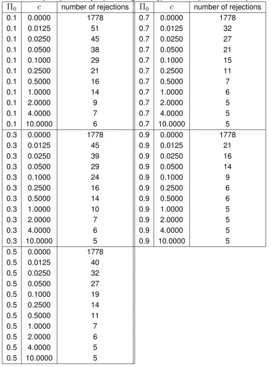
j equivalently amounts to a thresholding of these Bayes factors.

Table 3 lists the number of rejections (according to the decision rule defined in Proposition 1) as a function of

Π

0 and

c. As expected, the number of rejections is a decreasing function both of

c

and of

Π

0. If

c

= 0, then only the type II error component contributes to the risk

R(

d

,

data),

such that

R(

d

,

data)can trivially be optimized by rejecting all null hypotheses. However, as

c

increases, the number of rejections sharply decreases. This is the price that has to be paid for the high (effective) multiplicity of the problem, because

π

0

= Π

1/1350.450 is close to one for all

considered values of

Π

0. However, for the SNPs with the five smallest Bayes factors (namely

those which are smaller that

10

−5_{, see Table 2), the data overrule even large values of}

_Π

0and

c,

such that the corresponding five null hypotheses are rejected under any parameter configuration in Table 3.

6

Frequentist-Bayes reconciliation

The good accordance between frequentist

p-values and Bayes factors that we have reported

in Section 4 leads to the question if the frequentist and the Bayesian approach can be recon-ciled under our setup. To this end, Wakefield (2009) considered the saturated logistic regression model corresponding to the contigency table data for testing genetic associations. In an asymp-totic setting (N

→ ∞

), he derived a Gaussian prior for the regression coefficients which is guaranteed to lead to an ordering of the Bayes factors which coincides with that of frequentist

p-values.

Table 3: Number of rejected null hypotheses according to the decision rule from Proposition 1 as a function of the prior probability

Π

0 for the global hypothesis

H

0and the cost parameter

c.

Π

0

c

number of rejections

Π

0

c

number of rejections

0.1 0.0000 1778 0.7 0.0000 1778 0.1 0.0125 51 0.7 0.0125 32 0.1 0.0250 45 0.7 0.0250 27 0.1 0.0500 38 0.7 0.0500 21 0.1 0.1000 29 0.7 0.1000 15 0.1 0.2500 21 0.7 0.2500 11 0.1 0.5000 16 0.7 0.5000 7 0.1 1.0000 14 0.7 1.0000 6 0.1 2.0000 9 0.7 2.0000 5 0.1 4.0000 7 0.7 4.0000 5 0.1 10.0000 6 0.7 10.0000 5 0.3 0.0000 1778 0.9 0.0000 1778 0.3 0.0125 45 0.9 0.0125 21 0.3 0.0250 39 0.9 0.0250 16 0.3 0.0500 29 0.9 0.0500 14 0.3 0.1000 24 0.9 0.1000 9 0.3 0.2500 16 0.9 0.2500 6 0.3 0.5000 14 0.9 0.5000 6 0.3 1.0000 10 0.9 1.0000 5 0.3 2.0000 7 0.9 2.0000 5 0.3 4.0000 6 0.9 4.0000 5 0.3 10.0000 5 0.9 10.0000 5 0.5 0.0000 1778 0.5 0.0125 40 0.5 0.0250 32 0.5 0.0500 27 0.5 0.1000 19 0.5 0.2500 14 0.5 0.5000 11 0.5 1.0000 7 0.5 2.0000 6 0.5 4.0000 5 0.5 10.0000 5

As outlined in Section 4, one computationally very inexpensive method to transform

F

2to the

p-value scale is to apply the inverse transformation

[B(p)]

−1_{(Sellke et al. (2001)) to}

_F

2, provided

that

F

2 is smaller than

1. This leads to the upper

p-value bound

p(F

2

) =

−

F

2

e

×

LambertW(

−

1,

−

F

2

/e)

,

(9)

parameter

k

=

−

1, see

http://www.maplesoft.com/support/help/Maple/

view.aspx?path=LambertW

for details. The right-hand side of (9) is easily computable with standard statistics software. Since

B(p)

is a one-to-one mapping for

p

∈

(0, e

−1

_{), it is}

guaranteed that the order of the Bayes factors and that of the upper

p-value bounds defined by

(9) coincide. However, in terms of statistical significance, this approach is conservative, because

p(F

2

)

is an upper bound on the actual

p-value and may not be sharp.

Based on our considerations from Sections 1 and 2, a maybe more straightforward, albeit com-putationally very intensive approach towards the reconciliation problem consists in interpreting the Bayes factor as a statistic

F

2

:

X →

R

and carrying out a frequentist significance test

based on this test statistic. Let us briefly outline a simulation scheme for a Monte Carlo approx-imation of the distribution of

F

2 under

H

(Algorithm 1). For this, we denote by

f

2∗ the actually

observed value of the Bayes factor

F

2 at a given genetic locus based on the corresponding

contingency table

x

.

Algorithm 1.

0. Take

n

1.

, n

2., and

f

2∗ as input. Fix a number

B

MC of Monte Carlo repetitions. Initialize the

integer

counter

with

1

.

1. For

b

from

1

to

B

MCdo:

(a) Draw a pseudo-random number

a

(b)_{from the log-Cauchy}

_{(0, π)}

_{distribution.}

(b) Draw a pseudo-random tuple

(n

(b).1

, n

(b) .2

, n

(b)

.3

)

>from DMultinomial

(3, N, a

(b)

)

. This step

can for instance be performed by making use of the

MATLAB

routine

polya_sample.m

from the

Fastfit

toolbox by Thomas Minka.

(c) Draw a pseudo-random table

x

˜

(b)from the conditional distribution with point mass

func-tion

f

(

·|

n

(b)

)

, where

n

(b)

= (n

1.

, n

2.

, n

(b).1

, n

(b) .2

, n

(b) .3

)

>

. This step can be performed

efficiently by making use of the

AS 159

algorithm by Patefield (1981). A

MATLAB

implementation can be found under the URL

http://people.sc.fsu.edu/

~jburkardt/m_src/asa159/asa159.html

.

(d) Compute the Bayes factor

F

₂(b)based on

x

˜

(b). If

F

₂(b)

≤

f

∗

2, increase

counter

by

1

.

2. Return the relative frequency

ˆ

p

F2

(

x

) =

counter

B

MC

+ 1

.

(10)

The following result is an immediate consequence of the law of large numbers and the construc-tion of

p

ˆ

F2

(

x

).

Proposition 2.

(a) The quantity

p

ˆ

F2

(

x

)

defined in(10)consistently (

B

MC

→ ∞

) approximates the

frequen-tist

p

-value

p

F2

(

x

) =

P

(F

2

≤

f

∗ 2

|

H)

.

(b) The

p

-value

p

F2

(

x

)

is an increasing transformation of

f

∗ 2.

Remark 4. Notice that

p

ˆ

F2

(

x

)

cannot be smaller than

(B

MC

+ 1)

−1_{. In practice, one will}

there-fore typically have to choose

B

MC very large to ensure that

p

ˆ

F2

(

x

)

can possibly be smaller

than a multiplicity-adjusted significance threshold. Since the present paper proposes the usage of Bayesian decision theoretic multiple comparison procedures, we do not present numerical

values for the

p

ˆ

F2

(

x

(j)

₎

_,

₁

_≤

_j

_≤

_m

_{, here.}

7

Concluding remarks

We have presented an application in which Bayesian inference is easier and less computational demanding than (exact) frequentist inference. The main reason for this is that the parameter space stays constant with increasing sample size, while the cardinality of the sample space increases with

N

. Our approach enables the researcher to carry out decision theoretic multiple comparison procedures for testing genetic associations. Such procedures incorporate the prior probability for the validity of the global hypothesis as well as potentially non-symmetric costs for false decisions into the statistical methodology. Furthermore, we discussed several ways how to transform the proposed Bayes factors (which are very easy to compute in our setting) into

p-values, such that the ordering of both summary statistics with respect to the genetic loci under

investigation is the same.

There are several possible extensions of this work. First, recall that we considered a non-informative prior for the random column counts

(n

.1

, n

.2

, n

.3

)

>. However, in practice there will

often be prior information about the prevalence of the disease (the expected relative frequency of phenotype

1) and about the locus-specific allele frequencies in the target population.

Incor-porating this information into a different prior for

(n

.1

, n

.2

, n

.3

)

>is straightforward. Second, one

may incorporate linkage disequilibrium information not only in the construction of

M

eff., but more

explicitly in a probability model for

π

0(cf. Geisser (1984)) or for the observables themselves, as

proposed by Malovini et al. (2012). Third, it may be interesting to study the effect of the discrete-ness of

X

on the performance of decision theoretic multiple comparison procedures relying on posterior probabilities. In the frequentist context, Finner et al. (2010), Habiger and Peña (2011) and Dickhaus et al. (2012) have recently demonstrated that randomization techniques can in-crease the statistical power to detect true alternatives in discrete models. Finally, an interesting and challenging problem consists in adapting the concept of effective numbers of tests to the Bayesian context. There are at least two possible ways in this respect: One may analyze the equation

π

Meff.

0

= Π

0 under a probability model (with block dependencies) that explicitly

incor-porates the biological mechanism leading to LD, or one may replace the chi-square statistics considered by Moskvina and Schmidt (2008) and Dickhaus and Stange (2013) by Bayesian quantities, for instance by local false discovery rates as proposed by Yekutieli (2013).

Finally, one limitation of our approach in comparison to that of Wakefield (2009) is that non-genetic covariates are not included in our probability model. Future research shall aim at ex-tending the model such that adjustments for such covariates become possible.

References

Agresti, A. (2002):Categorical data analysis. 2nd ed., Wiley Series in Probability and Mathe-matical Statistics. Applied Probability and Statistics. Chichester: Wiley.

Agresti, A. and D. B. Hitchcock (2005): “Bayesian inference for categorical data analysis.”Stat.

Methods Appl., 14, 297–330.

Bakke, Ø. and M. Langaas (2012): “The number of

2

×

c

tables with given margins,” Statistics Preprint No. 11/2012, Norwegian University of Science and Technology, Trondheim.

Cheverud, J. M. (2001): “A simple correction for multiple comparisons in interval mapping genome scans.”Heredity, 87, 52–58.

Crook, J. and I. Good (1980): “On the application of symmetric Dirichlet distributions and their mixtures to contingency tables. II.”Ann. Stat., 8, 1198–1218.

Dawid, A. P. (1987): “The Difficulty About Conjunction,”Journal of the Royal Statistical Society,

Series D (The Statistician), 2/3, 91–97.

Dickhaus, T. (2014):Simultaneous Statistical Inference with Applications in the Life Sciences, Springer-Verlag Berlin Heidelberg.

Dickhaus, T. and J. Stange (2013): “Multiple point hypothesis test problems and effective num-bers of tests for control of the family-wise error rate,”Calcutta Statistical Association Bulletin, 65, 123–144.

Dickhaus, T., K. Strassburger, D. Schunk, C. Morcillo-Suarez, T. Illig, and A. Navarro (2012): “How to analyze many contingency tables simultaneously in genetic association studies,”

Stat Appl Genet Mol Biol, 11, Article 12.

Efron, B. (2010):Large-scale inference. Empirical Bayes methods for estimation, testing, and

prediction, Cambridge: Cambridge University Press.

Finner, H., K. Straßburger, I. M. Heid, C. Herder, W. Rathmann, G. Giani, T. Dickhaus, P. Lichtner, T. Meitinger, H.-E. Wichmann, T. Illig, and C. Gieger (2010): “How to link call rate and

p-values

for Hardy-Weinberg equilibrium as measures of genome-wide SNP data quality,”Statistics in

Medicine,, 29, 2347–2358.

Fisher, R. A. (1922): “On the interpretation of

χ

2_{from contingency tables, and the calculation of}

p,”Journal of the Royal Statistical Society, 85, 87–94.

Gao, X., J. Starmer, and E. R. Martin (2008): “A Multiple Testing Correction Method for Genetic Association Studies Using Correlated Single Nucleotide Polymorphisms.”Genetic

Epidemi-ology, 32, 361–369.

Geisser, S. (1984): “On prior distributions for binary trials.”Am. Stat., 38, 244–251.

Gómez-Villegas, M. and B. González-Pérez (2010): “r

×

s

tables from a Bayesian viewpoint.”

Good, I. (1976): “On the application of symmetric Dirichlet distributions and their mixtures to contingency tables.”Ann. Stat., 4, 1159–1189.

Habiger, J. D. and E. A. Peña (2011): “Randomised P-values and nonparametric procedures in multiple testing.”Journal of Nonparametric Statistics, 23, 583–604.

Langaas, M. and Ø. Bakke (2013): “Robust Methods for Disease-Genotype Association in Ge-netic Association Studies: Calculate

P

-values Using Exact Conditional Enumeration instead of Asymptotic Approximations,” arXiv:1307.7536v1.

León-Novelo, L. G., P. Müller, W. Arap, J. Sun, R. Pasqualini, and K.-A. Do (2013): “Bayesian decision theoretic multiple comparison procedures: An application to phage display data.”

Biom. J., 55, 478–489.

Lewontin, R. C. and K. I. Kojima (1960): “The evolutionary dynamics of complex polymorphisms,”

Evolution, 14, 458–472.

Lydersen, S., M. W. Fagerland, and P. Laake (2009): “Recommended tests for association in 2 x 2 tables,”Stat Med, 28, 1159–1175.

Malovini, A., N. Barbarini, R. Bellazzi, and F. de Michelis (2012): “Hierarchical Naive Bayes for genetic association studies,”BMC Bioinformatics, 13 Suppl 14, S6.

McCarroll, S. A., F. G. Kuruvilla, J. M. Korn, S. Cawley, J. Nemesh, A. Wysoker, M. H. Shapero, P. I. de Bakker, J. B. Maller, A. Kirby, A. L. Elliott, M. Parkin, E. Hubbell, T. Webster, R. Mei, J. Veitch, P. J. Collins, R. Handsaker, S. Lincoln, M. Nizzari, J. Blume, K. W. Jones, R. Rava, M. J. Daly, S. B. Gabriel, and D. Altshuler (2008): “Integrated detection and population-genetic analysis of SNPs and copy number variation,”Nat. Genet., 40, 1166–1174.

Moskvina, V. and K. M. Schmidt (2008): “On multiple-testing correction in genome-wide associ-ation studies,”Genetic Epidemiology, 32, 567–573.

Müller, P., G. Parmigiani, and K. Rice (2007): “FDR and Bayesian Multiple Comparisons Rules.”

inJ. M. Bernardo, M. J. Bayarri, J. O. Berger, A. P. Dawid, D. Heckerman, A. F. M. Smith and

M. West (eds.): Bayesian Statistics 8 - Proc. ISBA 8th World Meeting on Bayesian Statistics,

Oxford: Oxford University Press, 349–370.

Müller, P., G. Parmigiani, C. Robert, and J. Rousseau (2004): “Optimal sample size for multiple testing: the case of gene expression microarrays.”J. Am. Stat. Assoc., 99, 990–1001. Ng, K. W., G.-L. Tian, and M.-L. Tang (2011):Dirichlet and related distributions: Theory, methods

and applications., Hoboken, NJ: John Wiley & Sons.

Nyholt, D. R. (2004): “A simple correction for multiple testing for SNPs in linkage disequilibrium with each other.”Am. J. Hum. Genet., 74, 765–769.

Patefield, W. (1981): “An efficient method of generating random RxC tables with given row and column totals. (Algorithm AS 159.).”J. R. Stat. Soc., Ser. C, 30, 91–97.

Pearson, K. (1900): “On the criterion, that a given system of deviations from the probable in the case of a correlated system of variables is such that it can be reasonably supposed to have arisen from random sampling.”Phil. Mag. (5), 50, 157–175.

Scott, J. G. and J. O. Berger (2010): “Bayes and empirical-Bayes multiplicity adjustment in the variable-selection problem.”Ann. Stat., 38, 2587–2619.

Sellke, T., M. Bayarri, and J. O. Berger (2001): “Calibration of

p

Values for testing precise null hypotheses.”Am. Stat., 55, 62–71.

The 1000 Genomes Consortium (2010): “A map of human genome variation from population-scale sequencing,”Nature, 467, 1061–1073.

The International HapMap Consortium (2005): “A haplotype map of the human genome,” Na-ture, 437, 1299–1320.

The Wellcome Trust Case Control Consortium (2007): “Genome-wide association study of 14,000 cases of seven common diseases and 3,000 shared controls,”Nature, 447, 661–678. Wakefield, J. (2009): “Bayes factors for genome-wide association studies: comparison with

P-values,”Genet. Epidemiol., 33, 79–86.

Westfall, P. H., W. O. Johnson, and J. M. Utts (1997): “A Bayesian perspective on the Bonferroni adjustment.”Biometrika, 84, 419–427.

Yekutieli, D. (2013): “Optimal exact tests for composite alternative hypotheses on cross tabulated data,” arXiv:1310.0275v2.