An Improved Panel Unit Root Test Using
GLS-Detrending
Claude Lopez1
University of Cincinnati
Abstract
We propose to combine recent developments in univariate and mul-tivariate unit root testing in order to construct a more powerful panel unit root test. We extend the GLS-detrending procedure of Elliott, Rothenberg and Stock (1996) to a panel Augmented Dickey-Fuller test. The …nite sample power properties of the new test demonstrate a very large gain when compared to existing tests, especially for small panels. We then investigate the topic of Purchasing Power Parity for the post Bretton-Woods period via this new test. The results show strong rejections of the unit root hypothesis.
JEL classi…cation: C12, C15, C32, C33
1I am very grateful to David Papell and Chris Murray for helpful discussions and com-ments. I would like to thank Debashis Pal and the seminar participants at the University of Houston for encouragements and helpful suggestions. Claude Lopez, Assistant Profes-sor, Department of Economics - University of Cincinnati, 1209 Crosley Tower Cincinnati OH 45221-0371, Tel: 513-556-2346, Fax: 513-556-2669, Email: [email protected].
1
Introduction
Economic analysis of most time series requires stationarity of the data. Unit root tests are commonly used to address this matter. The most well-known among them is the augmented Dickey-Fuller (ADF) unit root test. Recent works, however have acknowledge the poor power properties of this test, which leads to a vast literature attempting to overcome these disadvantages. These developments have occurred at both multivariate and univariate levels. At the multivariate level, authors such as Levin, Lin and Chu (LLC) (2002), Im, Pesaran and Shin (1997) and Maddala and Wu (1996) o¤er excel-lent alternatives to the ADF test by combining time-series information with cross-sectional variability. The panel approach appears extremely appealing for two reasons. First, the inclusion of a limited amount of cross-sectional information induces signi…cant improvement in term of power. Second, the data needed for this type of analysis is increasingly available.
The LLC test and more speci…cally the LLC hypotheses are widely used. Indeed, several works propose enhanced versions of this test, producing data speci…c estimations. Papell (1997) suggests accounting for heterogeneous ser-ial correlation, while O’Connell (1998) demonstrates the necessity of allowing
for the cross-sectional dependence in the estimation procedure.2;3 Papell and Theodoridis (2001) incorporate both by considering a panel version of the ADF test, using the LLC hypotheses and allowing for heterogeneous serial and contemporaneous correlation.
At the univariate level, Elliott, Rothenberg and Stock (1996) develop a GLS-detrended/demeaned version of the ADF test. Running the ADF test on the GLS-transformed data leads to one of the most powerful univariate test,
which they call the DF-GLS test.4 While these innovations deliver substantial
gains in power over the univariate ADF test, they still demonstrate limited performance when applied to economic time-series data. Indeed, most of the data sets available have a limited length.
The present work intends to develop a new panel unit root test, o¤er-ing satisfyo¤er-ing performance especially in case of highly persistent series and limited amount of data. Seeking a signi…cant increase in power over exist-ing tests, we combine the GLS-detrendexist-ing of Elliott, Rothenberg and Stock (1996) with the panel ADF test, using Levin, Lin, and Chu’s (2002)
hypothe-2Papell (1997) shows a strong relation between the size of the panel and the rate of rejection of the unit root hypothesis.
3O’Connell (1998) points out the sizeable bias induced by the neglect of contempora-neous correlation when estimating cross-correlated data.
4Hansen (1995) proposes a more powerful alternative to the DF-GLS test by including covariates to the test, at the univariate level.
ses. We analyze the behavior of our panel unit root test for various sample sizes, panel widths, and degrees of persistence with a Monte Carlo experi-ment. The main result is that our panel unit root test displays signi…cantly better …nite sample power than existing univariate and panel unit root tests. We illustrate the test with an application to the Purchasing Power Parity (PPP) query within industrialized countries. We focus on the post Bretton-Woods period because neither the panel ADF test nor the DF-GLS test are able to reject the existence of a unit root. The principal outcome is a robust overall support for the PPP hypothesis, independently of the width and the length of the panels considered.
The next section provides a concise review of the literature that relates to the understanding of our proposed unit root test. Section 3 develops the new panel unit root test and tabulates the …nite sample critical values, while Section 4 conducts a detailed power experiment, where it is shown that the new test provides a signi…cant increase in power over the panel ADF test. Section 5 presents an empirical application to PPP, and, …nally, Section 6 summarizes our …ndings.
2
Existing Unit Root Tests: A Concise
Re-view of the Literature
In this section, we present the existing tests which have motivated this work and which help to its understanding. First, the standard ADF unit root test runs the following regression:
yt=dt+ yt 1 +
k
X
i=1
i yt i+ut (1)
where yt is the tested series, dt a set of deterministic regressors, k the
lagged …rst di¤erence terms allowing for serial correlation and ut the error
term of the regression. The unit root null hypothesis is that = 1, and
the alternative of stationarity is < 1. This test is well-known for its poor
power, and the subsequent literature suggests several solutions. In the next two subsections, we describe some recent developments at both multivariate and univariate levels.
2.1
More Powerful Unit Root Tests: Panel ADF Tests
The idea behind the panel unit root tests is to combine cross-sectional and time-series information to achieve a more e¢ cient test. Several panel pro-cedures have been developed to test the unit root null hypothesis against various alternative hypotheses. Levin, Lin, and Chu (2002) test the unit root null hypothesis against a homogenous alternative that every series in the panel is stationary with the same speed of reversion. Im, Pesaran and Shin (1997) and Maddala and Wu (1996) test the unit root null hypothesis against the alternative that at least one series in the panel is stationary. The new test, later proposed in this paper, focuses on the stationarity of the entire panel, which automatically leads us to concentrate on the LLC framework. The LLC test runs the following panel version of equation (1):
yjt =djt+ yj;t 1 +
kj
X
i=1
ji yj;t i+ujt (2)
where is the homogeneous rate of convergence of the panel. The null
hypothesis is that = 1 and the alternative is that < 1. For each series
j,j = 1; :::; N; dit = 0jzt is a set of deterministic regressors, which allows for
are included to account for serial correlation. The error terms are assumed
to be contemporaneously uncorrelated, E(uitujt) = 0 for i6=j.
While the LLC test leads to substantial improvements over the ADF test in terms of power, it is based on the extremely restrictive assumption that the series in the panel are cross-sectionally uncorrelated. Maddala and Wu (1996) and O’Connell (1998) demonstrate that if the error terms in equation (2) are indeed contemporaneously correlated, the LLC test exhibits severe
size distortions.5 As an alternative, Papell and Theodoridis (2001) estimate
the system of equations de…ned by (2) using Seemingly Unrelated Regressions (SUR). This version of the LLC test, which we refer to as the ADF-SUR test, accounts for serial and contemporaneous correlation. In the rest of this paper, we shall estimate equation (2) allowing for contemporaneous correlation.
Performing the ADF-SUR test is a two-step procedure. First, for each
series j,j = 1; :::; N, the number of lagged …rst di¤erence terms, kj, must be
selected to account for serial correlation. In this work, we use the general-to-speci…c (GS) lag-selection procedure of Hall (1994) and Ng and Perron (1995).
Then, having selected kj, the system of equations needs to be estimated via
SUR, constraining the values of to be identical across equations.
5O’Connell (1998) imposes homogeneous serial correlation properties across the series, which results in under rejection of the null hypothesis.
2.2
More Powerful Univariate Unit Root Tests: The
DF-GLS Test
Elliott, Rothenberg, and Stock (1996) construct an e¢ cient univariate unit root test based on local-to-unity asymptotic theory. The DF-GLS test is an ADF test on GLS-demeaned (or GLS-detrended) data. Speci…cally, the DF-GLS test runs the following regression:
The demeaned case, zt= (1):
yt = yt 1+
k
X
i=1
i yt i+ut (3)
The detrended case, zt= (1; t):
yt = yt 1+
k
X
i=1
i yt i+ut (4)
whereyt(yt)is the GLS-demeaned (GLS-detrended) series.
Equations (3) and (4) can be rewritten as:
ytGLS = ytGLS1 + k X i=1 i y GLS t i +ut , with GLS = ( ; ) (5)
of z~ on y~, i.e. ~ = (Pz~2
t)
1P
~
zty~t. y~tand z~t are the quasi-di¤erences of
yt and zt respectively, i.e. y~t = (y1;(y2 ay1); :::;(yT ayT 1))0, and z~t =
(z1;(z2 az1); :::;(zT azT 1))0. a = 1 +Tc represents the local alternative,
with c= 7 when zt = (1) and c = 13:5 when zt = (1; t).6 The standard
hypotheses are tested: H0 : = 1 versusH1 : <1.
The lag-selection issue in the DF-GLS regressions has received much at-tention recently. Ng and Perron (2001) propose a new lag selection proce-dure, the Modi…ed Akaike Information Criterion (MAIC), that provides the best combination of size and power in …nite samples when combined with
the GLS-transformation.7 In subsequent applications, we employ the MAIC
when performing the DF-GLS test.
6¯c = -7 ( ¯c= -13.5) corresponds to the tangency between the asymptotic local power function of the test and the power envelope at 50% power in the case with a constant (the case with a constant and a trend).
7MAIC takes into account the nature of the deterministic components and the de-meaning/detrending procedure, which allows a better measurement of the cost of each lag-length choice.
3
An Improved Panel Unit Root Test : The
DF-GLS-SUR Test
Both the ADF-SUR and the DF-GLS tests demonstrate higher power than the standard ADF test. They display, however, a limited ability to reject the unit root hypothesis for economic time series of the length generally encoun-tered in practice. Consequently, we propose to combine both innovations to obtain a more powerful unit root test. The new test, which we refer to as the
DF-GLS-SUR test, runs the following system of equations for j = 1; :::; N:
yGLSjt = yj;tGLS1 +
kj
X
i=1
i yj;t iGLS +ujt , with GLS = ( ; ) (6)
where is the homogeneous rate of convergence of the panel. The
stan-dard hypotheses are tested, that is H0 : = 1 versus H1 : <1.
The DF-GLS-SUR test requires a three-steps procedure. For each series
j, the data needs …rst to be GLS-transformed, thenkj, the number of lagged
…rst di¤erence terms allowing for serial correlation, must be selected using MAIC. Finally the system of equations is estimated via SUR, constraining
This procedure allows to test for the stationarity of the entire panel while accounting for data speci…c serial and contemporaneous correlation.
3.1
Finite Sample Critical Values
For the remaining of the paper, we consider the ADF-SUR test as benchmark. Even though Papell and Theodoridis (2001) use the ADF-SUR test, they do not report generic critical values. Therefore, we generate …nite sample critical values for both the ADF-SUR and the DF-GLS-SUR tests. The Monte Carlo
experiment considers panels with a length ofT = 25;50;75;100;and125;and
with a width of N = 5;10;15; and 20.8 The data sets are generated under
the null hypothesis as random walks without drift:
yjt =yj;t 1+uit (7)
whereujt~iidN(0;1)and the error terms are contemporaneously
uncorre-lated, E(uitujt) = 0 for i6=j.9
For each panel unit root test, we generate four sets of critical values. Two
8We consider T = 35;50;75;100;125 for the case with heterogeneous constants and trends.
9In the subsequent empirical exercise, we shall explicitly allow for contemporaneously correlated errors.
sets for each model (regressions with a constant only, and with a constant and a trend). First, we assume that the true lag-length is known, that is
we …x k = 0. We are also interested in the e¤ects of lag-length selection on
the …nite sample distribution of the unit root test statistics. Accordingly, we generate critical values where at each iteration we select the lag length by GS for the ADF-SUR test and by MAIC for the DF-GLS-SUR test.
Our results are consistent with the fact that the inclusion of serial corre-lation, selected via the GS procedure, induces a strong increase in absolute
value of the critical values.10 Furthermore, the percentage change in critical
values is more severe for the ADF-SUR test than for the DF-GLS-SUR test, i.e. when the lag length is selected via GS instead of via MAIC. The true
value of k being0and the MAIC procedure providing the best estimation of
the lag length, the critical values for both cases, k = 0 and k = kM AIC, are
relatively close.
The 1%, 5%, and 10% critical values are reported in Tables 1 and 3 for
the ADF-SUR test, and Tables 2 and 4 for the DF-GLS-SUR test.
4
Finite Sample Performances: Power
Analy-sis
Being a combination of the ADF-SUR and the DF-GLS tests, we expect the DF-GLS-SUR test to be more powerful than each one of them. Therefore,
we compute the power of the ADF-SUR and the DF-GLS-SUR tests.11
Con-sidering the same panels (N, T) than for the critical values, the power is computed via a Monte Carlo experiment with the data generated under the alternative, that is:
yit = yj;t 1+ujt (8)
whereujt~iidN(0;1), E(uitujt) = 0for i6=j and <1. We consider the
following alternatives = (0:99;0:97;0:95;0:90;0:85;0:80);with the nominal
size …xed at 5%. Tables 5, 6, 7, and 8 display the level of power for the
ADF-SUR and the DF-GLS-ADF-SUR tests, for the(k= 0)and the(k = (kGS; kM AIC))
cases using regressions with a constant only ( Tables 5 and 6) or with a
constant and a trend (Tables 7 and 8).
Below, we discuss three aspects of the results for both tests: a change
11Elliott, Rothenberg, and Stock (1996) provide the power analysis for the DF-GLS test for both demeaned and detrended cases.
in T, the length of the panel, a change in N, the width of the panel, and a decrease in , the persistence of the series.
4.1
Demeaned case:
Tables 5
and
6
A comparison between the power of the GLS-SUR test and of the DF-GLS test demonstrates that the inclusion of few more series to the univariate
DF-GLS test leads to drastic power improvements: for = 0:95andT = 100,
the power of the DF-GLS test is equal to 0:26, while for the DF-GLS-SUR
test the power is 0:98, with N = 5.
Commonly, the lag selection induces a uniform power loss, compared to the case where the lag length is known and equal to 0. The simulations show
this expected outcome, with Table 6 having a lower power than Table 5.
Except for this di¤erence, however, Tables 5 and 6 present similar patterns:
the DF-GLS-SUR test demonstrates an overall higher power than the ADF-SUR test. Therefore, unless it is clearly speci…ed, the following performance analysis does not dissociate these two cases.
A sole increase in T leads to consistent increases in power for both tests with signi…cantly stronger improvements for the DF-GLS-SUR test than the ADF-SUR test. For example, considering the case with no lags, a highly
persistent system of series, = 0:99, a limited amount of series, N = 5, and a small increase in the length of the panel, T varies from 25 to 50 observations, the DF-GLS-SUR test produces an increase in power ten times
higher than the ADF-SUR test. The same case with a wider panel (N = 20),
demonstrates a similar outcome. For highly persistent series with a small number of observations, the DF-GLS-SUR test o¤ers higher power than the ADF-SUR test, and takes better advantage of an increase in T.
For less persistent processes, for example = (0:97;0:95), the
DF-GLS-SUR test continues to present a stronger response to an increase in the num-ber of observations than the ADF-SUR test.
A sole increase in N leads to consistent power improvements, with a stronger impact on the DF-GLS-SUR test than on the ADF-SUR test. For
example, with lag-length selection, = 0:99, and T = 25, an increase in
the number of series, N evolving from 5 to 10, leads to a power increase for the DF-GLS-SUR test …ve times stronger than for the ADF-SUR test. Fur-thermore, if we compare the impact of a change in T with the impact of a change in N, the tables show for both tests that an increase in width has a stronger e¤ect than an increase in length. Considering the case with no lags
A minimum of 50 observations needs to be added to reach a power level close to 1, while the addition of only 5 series displays the similar result.
(N; T) = (20;50) presents an interesting case, especially if the processes are highly persistent. The ADF-SUR test is well-known for its power de-…ciency when the width and the length of the panel are too close. In the
presence of lags, and with = 0:99, this combination presents a power of
0.44 for the DF-GLS-SUR test and of 0.10 for the ADF-SUR test. If = 0:97,
the DF-GLS-SUR test reaches a power of 0.98 while the ADF-GLS test of-fers only a power of 0.22. The DF-GLS-SUR test demonstrates an impressive higher power than the ADF-SUR test for panels including highly persistent series and with a width close to the length.
As expected, a change in the series persistence also has a major in‡uence on the behavior of both the DF-GLS-SUR and the ADF-SUR tests. In the
case with lags, and(N; T) = (10;75), the DF-GLS-SUR test presents a power
of 0.41 for = 0:99, of 0.98 for = 0:97 and of 1.00 for = 0:95. More
generally, the DF-GLS-SUR test has a power of 1.00 or close to 1.00 whenever
4.2
Detrended case:
Tables 7
and
8
Commonly, the addition of a trend to the regressions leads to a uniform loss
in power for both tests: with = 0:97and (N; T) = (15;100), the
DF-GLS-SUR test produces a power of 1.00 while the DF-GLS-DF-GLS-SUR test reaches
only a power of 0.30.12 However, combining time-series information with
cross-sectional information still provides signi…cant improvements in the test
performance. For = 0:95 and T = 100, the DF-GLS test reaches a power
level of 0.10 while the DF-GLS-SUR test, accounting for four more series
(N = 5), is able to achieve a power level of 0.35.
The GLS-transformation shows a similar impact on the size-adjusted
power than in Section 3. If = 0:95and(N; T) = (5;125), the DF-GLS-SUR
test has a power of 0.53 while the ADF-SUR test o¤ers a power level of 0.24. Furthermore, the amplitude of these enhancements varies following changes
in T, inN or in , as well as the test considered. For = 0:97 and N = 20,
a raise in T from 50 to 100 observations induces an power increase of 0.23
for the DF-GLS-SUR test and of 0.10 for the ADF-SUR test. Likewise, if N
varies from 15 to 20 series, when = 0:97and T = 100, the power augments
12The DF-GLS-SUR test refers to the demeaned case while the DF-GLS-SUR refers to the detrended case.
by 0.32 for the DF-GLS-SUR test and by 0.03 for the ADF-SUR test. Finally,
a decrease in the persistence, from = 0:97 to = 0:95, generates strong
improvements in the performance for both tests: for (N; T) = (10;125), the
observed power increase is of 0.45 for the DF-GLS-SUR test and of 0.25 for the ADF-SUR test.
To sum up, this analysis reveals two major outcomes. First, as expected, by incorporating cross-sectional variation we are able to signi…cantly en-hance the power of the univariate DF-GLS test. Secondly, the comparison of both test performances demonstrates strong improvements due to the GLS-transformation. Overall the DF-GLS-SUR test has a higher …nite sample power than the ADF-SUR test, and for each increase in information (either
N orT), the corresponding increase in power is larger for the DF-GLS-SUR
test than the ADF-SUR test. Furthermore, our new test presents some inter-esting features: its power is attractively high for small panels and for highly persistent series.
4.3
Robustness Analysis
One obvious objection to this new test stands in the homogeneity imposed by the alternative hypothesis. This restriction seems to undermine the enhanced
power properties previously presented. Consequently, in this section, we focus on the impact of such a constraint by measuring the performance of the DF-GLS-SUR test when applied to series with heterogeneous rates of convergence. Our results show that, even under such conditions, the DF-GLS-SUR test remains one of the most powerful unit root tests available.
We proceed with the Monte Carlo experiment de…ned earlier for the power analysis, but allowing for the rate of convergence to vary across the generated series, i.e. the data generating process follows:
yjt = jyj;t 1+ujt (9)
where ujt~iidN(0;1), E(uitujt) = 0 for i 6= j;and j 1. Then we
estimate equation (3) with k= 1.13
Due to the in…nite number of cases existing, we focus on the six subse-quent panels:
N = 5, T = (50;100) and j is divided in two groups such that i = (1:00;0:99;0:97;0:95;0:90;0:85;0:80) fori = 1;2;3and l= (1:00;0:99;0:97, 0:95;0:90;0:85;0:80) for l = 4;5.
13This allows us to compare the size-adjusted power with Bowman (1999) and Im, Pesaran and Shin (1997).
N = 15, T = (50;100) and j is divided in three groups such that i = (1:00;0:99;0:97;0:95;0:90;0:85;0:80)fori= 1;2;3;4;5, l= (1:00;0:99;0:97, 0:95;0:90;0:85;0:80) for l = 6;7;8;9;10 and m = (0:80;0:95) for m = 11;12;13;14;15.
The size-adjusted power resulting from these simulations is reported in
Figure 1.
The 3D graphs demonstrate strong deteriorations in the DF-GLS-SUR-test performance in presence of random walks among the series. For example, if(N; T) = (5;50)and = (1:00;0:99), the power level reached is 0.08 instead
of 0.18 when i = j = 0:99. Power losses are also observed when some of
the series estimated include processes more persistent than the alternative
considered in the homogeneous case: if (N; T) = (15;50), the DF-GLS-SUR
test achieves a power of 0.88 when ( i; j; m) = (0.97,0.99,0.80), instead of
1.00 when i = j = m = 0:80. The converse is also veri…ed: if( i; j; m) =
(0:85;0:90;0:95)the power equals 1.00, while if i = j = m = 0:95it equals
0.99.
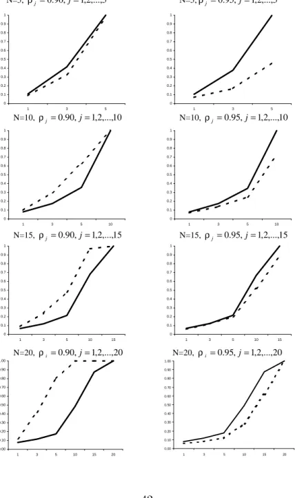
The relatively poor performance of the DF-GLS-SUR test in presence of non-stationary processes encourages a comparison with the Im, Pesaran and
X-axis represents the number of stationary series among the panel and the
Y-axis is the power. The panels considered have a width ofN = 5;10;15;20
and a length …xed to T = 100. The rates of convergence for the stationary
processes are = (0:90;0:95).
Overall, the DF-GLS-SUR test demonstrates a higher power than the
IPS test when = 0:95. These results imply that, in highly persistent
cases, the impact of GLS-transformation prevails over the negative e¤ect of the homogeneous alternative on the test performance. Our …ndings con…rm that the GLS-transformation improves the …nite sample power properties of the test, especially when investigating mixes of highly persistent and non-stationary series, even though the alternative hypothesis is wrong.
The DF-GLS-SUR test alternative hypothesis has a limited impact on the test performance in presence of series converging at di¤erent rates, but rather a strong and negative e¤ect when the panel combines stationary and non-stationary processes. However, the latter observation has limited e¤ects on the test reliability. Indeed, the DF-GLS-SUR test focuses on the stationarity
of the entire panel: the presence of at least one unit root should lead to no
rejection of the null hypothesis.14
14Di¤erently, the IPS test is supposed to reject the unit root hypothesis if at least one process in the panel is stationary.
To sum up, the DF-GLS-SUR test was designed to answer more accu-rately whether or not the panel converges. Its overall satisfying performance in presence of homogeneous or heterogeneous rates of convergence in a sta-tionary data set con…rms its accuracy. Furthermore, the relatively low power achieved in presence of random walks in the panel is not a major issue because
it is still signi…cantly higher than the nominal size (5%).15
5
Illustration: Purchasing Power Parity
As an illustration, we apply this new test to the Purchasing Power Par-ity (PPP) query. We consider quarterly CPIs and nominal exchange rates in dollars, from 1973(1), …rst quarter, to 1998(2), second quarter, (Source IFS, CD-Rom for 03/2002), for 21 industrialized countries: Australia, Aus-tria, Belgium, Canada, Denmark, Finland, France, Germany, Greece, Ireland, Italy, Japan, Netherlands, Norway, New Zealand, Portugal, Spain, Sweden, Switzerland, the U.K., and the U.S..We then construct the corresponding
15The only issue could be to over-reject the null hypothesis but by controlling for the size, i.e. the tendency to over-reject the null, we solve this issue as long as the power is signi…cantly higher than the size.
real exchange rate, qj (in logarithm) follows:
qj =ej +p pj (10)
whereej,pj and p are the logarithm of the nominal exchange rate (U.S.
dollar as numeraire), the foreign CPI and the US CPI.
We …rst proceed with univariate estimations of the real exchange rates through the ADF and the DF-GLS tests, using as lag-length selection the
GS and the MAIC procedures respectively. The results are shown inTable 9.
Few rejections of the unit root hypothesis are observed: the ADF test never rejects while the DF-GLS test o¤ers several rejections, varying from a 10% level for Denmark and Italy to a 5% level for Belgium, France, Germany, Greece and the Netherlands.
Next, we estimate the real exchange rates at the multivariate level with the ADF-SUR and the DF-SUR-GLS tests. The ADF-SUR test is a version of the LLC test accounting for contemporaneous correlation. The inclusion of correlation among the errors invalidates the limit distribution of the LLC
test.16 Maddala and Wu (1996) propose a bootstrapping alternative, and
16Maddala and Wu (1996), Banerjee (1999), Bowman (1999), and Chang (2002) point out this issue.
demonstrate that the LLC test o¤ers good performances when this technique is used. Therefore a Monte Carlo experiment is employed, allowing us to
generate the critical values under the standard hypotheses, i.e. H0 : = 0
versus H1 : <0.
Section 4, we have described the estimation process as well as the Monte Carlo experiment used to generate critical values. However, the data gener-ating process used for the nonspeci…c analysis did not include cross-sectional correlation. For the data-speci…c critical values, we need to estimate them by estimating the non-diagonal variance-covariance matrix of the innovations.
The jth real exchange rate, j = 1; :::; N, follows:
qjt =djt+ jqj;t 1+ujt (11)
whereujt = juj;t 1+ jt with ( 1t::: N t)0~N(0N; )and E(uitujt)6= 0 for
i6=j.
We …rst run ADF regressions for each series, using Schwarz information criteria lag selection in order to estimate the characteristics of each process. Those estimates are assumed to de…ne the true data generating processes
matrix of the innovations, i.e. (u1t:::unt)~N(0N; ). The unit root is
im-posed in the generated process by taking partial sums. Finally, we proceed with the rest of the Monte Carlo experiment: for each process the estimation
of equation(3)((1)) selects kM AIC
j (kGSj ), then equation(6)((2)) is estimated
using SUR, with the pre-selected kM AIC
j (kjGS).17 Repeating each procedure
5000 times creates a vector of statistics. Then the critical values are calcu-lated.
The data is grouped such that the panel of the 20 U.S.-real exchange rates (All20) includes Australia, Austria, Belgium, Canada, Denmark, Fin-land, France, Germany, Greece, IreFin-land, Italy, Japan, Netherlands, Norway, New Zealand, Portugal, Spain, Sweden, Switzerland, and the U. K. Then we consider the following panels: the European Community (EC), the Eu-ropean Monetary System (EMS), the 6 and 10 most industrialized countries (G6, G10), the Euro area as of 1999 (E10), the Euro area as of 2001 (E11),
and the OECD countries (13).18 For each panel, Table 10 reports the
esti-17We consider the case with constants only because we focus on the mean-reverting behavior of the real exchnage rates.
18EC includes Belgium, Denmark, France, Germany, Greece, Ireland, Italy, the Nether-lands, Portugal, Spain, and the U.K. EMS includes Belgium, Denmark, France, Germany, Ireland, Italy, and the Netherlands. G6 includes Canada, France, Germany, Italy, Japan, and the U.K. For G10, Belgium, the Netherlands, Sweden, and Switzerland are added. E11 includes Austria, Belgium, Finland, France, Germany, Greece, Ireland, Italy, the Nether-lands, Portugal, and Spain. E10 does not include Greece. 13 includes Australia, Belgium, Canada, Denmark, Finland, France, Germany, Italy, the Netherlands, Norway, Sweden,
mated , the t-statistic and the corresponding half-life (HL ) for the period 1973(1) 1998(2).19
The panels considered vary in size with a width including between 6 and 20 US-real exchange rates and a length of 102 observations. As shown in the performance analysis, the DF-GLS-SUR test demonstrates an high power for these speci…c cases (a minimum power level of 90%) while the ADF-SUR test behaves poorly, at least for the small panels (a power level of 20%). For the studied panels, the bias of the DF-GLS-SUR test is negligible compared to the bias of the ADF-SUR test. Furthermore, the high power observed for the DF-GLS-SUR test combined with a size …xed at 5% implies that the results strongly re‡ect the information available in the data.
The DF-GLS-SUR test demonstrates uniformly stronger rejections, with 7 rejections at 1% and 1 at 5% while the ADF-SUR test shows a majority of
rejection at 5% or less.20 By using a more powerful alternative to the existing
tests, we are able to produce the strongest evidence of PPP for the ‡oating period.
and the U.K.
19We calculate the half-life based on , that isHL =ln 0:5 ln .
20However, the DF-GLS-SUR test generates larger half-lives than the ADF-SUR test. Studies such as Murray and Papell (2002), and Lopez, Murray and Papell (2003) produce similar results.
6
Conclusion
The literature already provides several more powerful alternatives to the ADF unit root test. However, all of them demonstrate limited ability to reject correctly the unit root hypothesis when applied to highly persistent time series with a limited span. This paper attempts to produce a more e¢ -cient panel unit root test allowing a more reliable analysis of such data sets. Our new test, the DF-GLS-SUR test, is an extension of Elliott, Rothenberg, and Stock’s (1996) GLS-transformation to a version of the Levin, Lin and Chu’s (2002) test. The use of Monte Carlo simulations allow us to show the interesting behavior of this new test. For both the demeaned and de-trended cases, the DF-GLS-SUR test o¤ers a uniformly higher …nite-sample power than the ADF-SUR test. Furthermore, the DF-GLS-SUR-test perfor-mance remains attractive when studying a data with heterogeneous rates of convergence across the series.
The most pertinent feature of the DF-GLS-SUR test stands in its satis-fying power when applied to highly persistent processes with limited amount of observations. Indeed, it is always a challenge to increase signi…cantly the time-series dimension of economic data while the cross-sectional dimension is easily extendable.
References
Banerjee, A., 1999, Panel Data Unit Root and Cointegration: An Overview, Oxford Bulletin of Economics and Statistics, 61, 607-629.
Bowman, D., 1999, E¢ cient Tests for Autoregressive Unit Roots in Panel Data, International Finance Discussion Papers, number 646.
Chang, Y., 2002, Bootstrap Unit Root in Panels with Cross-Sectional De-pendency, Journal of Econometrics, forthcoming.
Elliott, G., T. Rothenberg, and Stock, J.H., 1996, E¢ cient Tests for an Autoregressive Unit Root, Econometrica, 64, 813-836.
Hall, A., 1994, Testing for a Unit Root in Time Series with Pretest Data-Based Model Selection, Journal of Business and Economic Statistics, 12, 461-470.
Hansen, B. E., 1995, Rethinking the Univariate Approach to Unit Root Test-ing: Using Covariates to Increase Power, Econometric Theory, 11, 1148-1172.
Im, K.S., M.H. Pesaran, and Y. Shin, 1997, Testing for Unit Roots in Het-erogeneous Panels (University of Cambridge).
Levin, A., C.F. Lin, and C.J. Chu, 2002, Unit Root Tests in Panel Data: Asymptotic and Finite-Sample Properties, Journal of Econometrics, 108, 1-24.
Lopez, C., Murray C.J., and D.H. Papell, 2002, State of the Art Unit Root Tests and the PPP Puzzle (University of Houston).
Maddala, G.S. and S. WU, 1996, A comparative Study of Unit Root Tests with Panel Data and a New Simple Test: Evidence from Simulations and Bootstrap (Ohio State University).
Murray, C.J., and D.H. Papell, 2002, The Purchasing Power Parity Persis-tence Paradigm, Journal of International Economics, 56, 1-19.
Ng, S., and P. Perron, 1995, Unit Root Test in ARMA Models with Data Dependent Methods for the Selection of the Truncation Lag, Journal of the American Statistical Association, 90, 268-281.
Ng. S., and P. Perron, 2001, Lag Length Selection and the Construction of Unit Root Tests with Good Size and Power, Econometrica, 69, 1519-1554.
O’Connell P., 1998, The Overvaluation of Purchasing Power Parity, Journal of International Economics, 44, 1-19.
Papell, D.H., 1997, Searching for Stationarity: Purchasing Power Parity un-der the Current Float, Journal of International Economics, 43, 313-332.
Papell, D.H., and H. Theodoridis, 2001, The Choice of Numeraire Currency in Panel Tests of Purchasing Power Parity, Journal of Money, Credit and Banking, 33, 790-803.
T a b le 1 : F in it e S a m p le C ri ti ca l V a lu es fo r th e A D F -S U R T es t, z= (1 ) N T 1% 5% 10% k =0 k =0 k =0 5 25 -5.6707 -7.2479 -4.8651 -6.1155 -4.4903 -5.5355 50 -5.2441 -5.8627 -4.5867 -5.1077 -4.2463 -4.6495 75 -5.0430 -5.4978 -4.4447 -4.7705 -4.1315 -4.4324 100 -5.0184 -5.3612 -4.4298 -4.6821 -4.1170 -4.3136 125 -4.9788 -5.2008 -4.3978 -4.5648 -4.1079 -4.2351 10 25 -7.6518 -9.3829 -6.6882 -8.1226 -6.2560 -7.4331 50 -6.6553 -7.3540 -6.0092 -6.5780 -5.6690 -6.1478 75 -6.4209 -6.8628 -5.7586 -6.1366 -5.4237 -5.7433 100 -6.2951 -6.5348 -5.6789 -5.9484 -5.3702 -5.6094 125 -6.2544 -6.5169 -5.6366 -5.8687 -5.3230 -5.5030 15 25 -10.4550 -11.5438 -9.1043 -10.1968 -8.3837 -9.5094 50 -7.9136 -8.6581 -7.2513 -7.8649 -6.8559 -7.4345 75 -7.5525 -8.0338 -6.8655 -7.2639 -6.5137 -6.8718 100 -7.2861 -7.6344 -6.7148 -7.0169 -6.3795 -6.6551 125 -7.2301 -7.5393 -6.7228 -6.8976 -6.3569 -6.5463 20 25 -50 -9.3641 -10.2436 -8.4795 -9.1318 -8.0607 -8.6413 75 -8.5003 -8.9527 -7.8859 -8.2686 -7.5369 -7.8973 100 -8.2865 -8.7111 -7.7323 -8.0245 -7.3488 -7.6499 125 -8.1448 -8.4751 -7.5264 -7.7635 -7.1730 -7.3898 GS k k = GS k k = GS k k =
T a b le 2 : F in it e S a m p le C ri ti ca l V a lu es fo r th e D F -G L S -S U R T es t, z= (1 ) N T 1% 5% 10% k =0 k =0 k =0 5 25 -3.1576 -3.5736 -2.3489 -2.6501 -1.9262 -2.1687 50 -2.9406 -2.9617 -2.2707 -2.3190 -1.8473 -1.9156 75 -2.8451 -2.8570 -2.2057 -2.2081 -1.8601 -1.8896 100 -2.8089 -2.8238 -2.1433 -2.1820 -1.7854 -1.8192 125 -2.7992 -2.7987 -2.1297 -2.1258 -1.7666 -1.7813 10 25 -3.6376 -3.9895 -2.7942 -3.0074 -2.2337 -2.4728 50 -3.1048 -3.2857 -2.4295 -2.5088 -2.0350 -2.1203 75 -3.1182 -3.1464 -2.3658 -2.4636 -1.9687 -2.0469 100 -2.9855 -2.9702 -2.3049 -2.3375 -1.8906 -1.9548 125 -2.9169 -2.9290 -2.2864 -2.3249 -1.9417 -1.9620 15 25 -4.5752 -4.7473 -3.3616 -3.5269 -2.7309 -2.9017 50 -3.4798 -3.5937 -2.6615 -2.7977 -2.2484 -2.3617 75 -3.3142 -3.3346 -2.5281 -2.6392 -2.1707 -2.2413 100 -3.1826 -3.2989 -2.4966 -2.5599 -2.0692 -2.1302 125 -3.1182 -3.1900 -2.3693 -2.3957 -2.0246 -2.0595 20 25 -50 -3.8437 -3.9963 -2.9495 -3.1214 -2.4988 -2.6501 75 -3.5204 -3.6599 -2.7059 -2.8150 -2.3362 -2.4182 100 -3.3528 -3.4175 -2.5408 -2.6331 -2.1907 -2.2403 125 -3.1817 -3.2041 -2.5374 -2.6082 -2.1950 -2.2489 M AIC k k = M AIC k k = M AIC k k =
T a b le 3 : F in it e S a m p le C ri ti ca l V a lu es fo r th e A D F -S U R T es t, z= (1 ,t ) N T 1% 5% 10% k =0 k =0 k =0 5 35 -6.9862 -9.9797 -6.3261 -8.6032 -5.9711 -7.9052 50 -6.7121 -7.8731 -6.1253 -7.1001 -5.7737 -6.6813 75 -6.4433 -7.2291 -5.9397 -6.5950 -5.6530 -6.2486 100 -6.4847 -7.0777 -5.9368 -6.4079 -5.6393 -6.0715 125 -6.3935 -6.9050 -5.8432 -6.2775 -5.5704 -5.9402 10 35 -9.3890 -12.9343 -8.6539 -11.4676 -8.3111 -10.7788 50 -8.8541 -10.4200 -8.2646 -9.5357 -7.9407 -9.0788 75 -8.5459 -9.4320 -7.9619 -8.7541 -7.6502 -8.4123 100 -8.4465 -9.1381 -7.8478 -8.4828 -7.5839 -8.1482 125 -8.2961 -8.9418 -7.7640 -8.2326 -7.4833 -7.9433 15 35 -11.6544 -16.3897 -10.7663 -14.5835 -10.4220 -13.7604 50 -10.7395 -12.3456 -10.1020 -11.5615 -9.7999 -11.0971 75 -10.2063 -11.3239 -9.6669 -10.5951 -9.3861 -10.2325 100 -10.0315 -10.8169 -9.4767 -10.1849 -9.1507 -9.8115 125 -9.8206 -10.4819 -9.3496 -9.8900 -9.0727 -9.5505 20 35 -50 -12.5861 -14.5574 -11.9055 -13.6222 -11.5147 -13.1007 75 -11.7610 -12.9922 -11.2252 -12.2593 -10.8897 -11.8815 100 -11.4545 -12.2848 -10.8657 -11.6550 -10.5851 -11.2859 125 -11.3289 -11.9535 -10.7024 -11.3388 -10.4153 -11.0085 GS k k = GS k k = GS k k =
T a b le 4 : F in it e S a m p le C ri ti ca l V a lu es fo r th e D F -G L S -S U R T es t, z= (1 ,t ) N T 1% 5% 10% k =0 k =0 k =0 5 35 -5.6655 -6.1837 -6.0890 -5.6667 -5.7906 -5.3943 50 -5.4555 -5.7931 -5.3722 -4.8815 -5.0888 -4.6203 75 -5.1615 -5.5635 -5.0796 -4.7250 -4.8120 -4.4606 100 -5.0973 -5.4424 -4.9069 -4.6111 -4.6513 -4.3884 125 -5.0596 -5.3895 -4.8384 -4.5767 -4.5512 -4.3201 10 35 -7.4675 -8.1771 -8.3094 -7.7066 -8.0535 -7.4251 50 -7.0952 -7.6604 -7.1533 -6.5814 -6.9261 -6.3123 75 -6.7551 -7.2354 -6.7399 -6.2724 -6.4708 -6.0011 100 -6.5987 -6.9806 -6.4973 -6.1126 -6.2131 -5.8673 125 -6.4887 -6.8641 -6.3360 -5.9645 -6.0661 -5.7220 15 35 -9.2049 -9.8818 -9.2049 -9.3956 -8.3701 -9.1696 50 -8.4095 -9.1628 -8.6821 -7.9467 -8.4536 -7.6964 75 -7.9856 -8.6046 -8.0940 -7.4962 -7.8286 -7.2521 100 -7.7685 -8.1982 -7.7327 -7.2597 -7.4862 -7.0184 125 -7.6625 -8.0551 -7.5585 -7.1493 -7.2943 -6.8944 20 35 -50 -10.5111 -9.7688 -10.0582 -9.2706 -9.8306 -9.0317 75 -9.7579 -9.1550 -9.2963 -8.6639 -9.0418 -8.4335 100 -9.3108 -8.8193 -8.8340 -8.3454 -8.5908 -8.1195 125 -9.0688 -8.6311 -8.5981 -8.1462 -8.3455 -7.9277 M AIC k k = M AIC k k = M AIC k k =
T a b le 5 : S iz e-A d ju st ed P o w er fo r th e A D F -S U R a n d th e D F -G L S -S U R T es ts , z= (1 ), n o la g s N T 0.99 0.97 0.95 0.90 0.85 0.80 ADF-SUR DF-GLS-SUR ADF-SUR DF-GLS-SUR ADF-SUR DF-GLS-SUR ADF-SUR DF-GLS-SUR ADF-SUR DF-GLS-SUR ADF-SUR DF-GLS-SUR 5 25 0.0588 0.1246 0.0726 0.2836 0.0870 0.4434 0.1660 0.7968 0.3036 0.9462 0.4998 0.9906 50 0.0646 0.1782 0.1002 0.5596 0.1668 0.8286 0.5156 0.9968 0.8618 0.9998 0.9884 1.0000 75 0.0848 0.2814 0.1810 0.8032 0.3562 0.9752 0.8812 1.0000 0.9984 1.0000 1.0000 1.0000 100 0.0868 0.3766 0.2310 0.9422 0.5342 0.9980 0.9894 1.0000 1.0000 1.0000 1.0000 1.0000 125 0.1082 0.4718 0.3426 0.9700 0.7400 1.0000 0.9994 1.0000 1.0000 1.0000 1.0000 1.0000 10 25 0.0622 0.1686 0.0750 0.4646 0.1022 0.7112 0.2132 0.9708 0.4422 0.9980 0.7128 1.0000 50 0.0720 0.3460 0.1410 0.8894 0.2790 0.9944 0.7956 1.0000 0.9914 1.0000 1.0000 1.0000 75 0.1028 0.5052 0.2688 0.9860 0.5876 1.0000 0.9942 1.0000 1.0000 1.0000 1.0000 1.0000 100 0.1160 0.6710 0.4136 0.9996 0.8474 1.0000 1.0000 1.0000 1.0000 1.0000 1.0000 1.0000 125 0.1440 0.7832 0.5970 1.0000 0.9664 1.0000 1.0000 1.0000 1.0000 1.0000 1.0000 1.0000 15 25 0.0542 0.2198 0.0674 0.5932 0.0778 0.8280 0.1454 0.9954 0.2866 0.9998 0.5420 1.0000 50 0.0794 0.4666 0.1718 0.9730 0.3614 0.9998 0.9148 1.0000 0.9990 1.0000 1.0000 1.0000 75 0.1154 0.6906 0.3624 0.9996 0.7494 1.0000 0.9994 1.0000 1.0000 1.0000 1.0000 1.0000 100 0.1456 0.8178 0.5812 1.0000 0.9528 1.0000 1.0000 1.0000 1.0000 1.0000 1.0000 1.0000 125 0.1556 0.9350 0.9904 1.0000 0.9938 1.0000 1.0000 1.0000 1.0000 1.0000 1.0000 1.0000 20 25 -50 0.0896 0.5578 0.1860 0.9912 0.4044 1.0000 0.9538 1.0000 1.0000 1.0000 1.0000 1.0000 75 0.1284 0.7998 0.4342 1.0000 0.8456 1.0000 1.0000 1.0000 1.0000 1.0000 1.0000 1.0000 100 0.1506 0.9350 0.6366 1.0000 0.9808 1.0000 1.0000 1.0000 1.0000 1.0000 1.0000 1.0000 125 0.2092 0.9772 0.7294 1.0000 1.0000 1.0000 1.0000 1.0000 1.0000 1.0000 1.0000 1.0000 = ρ
T a b le 6 : S iz e-A d ju st ed P o w er fo r th e A D F -S U R a n d th e D F -G L S -S U R T es ts , z= (1 ), w it h la g s N T 0.99 0.97 0.95 0.90 0.85 0.80 ADF-SUR DF-GLS-SUR ADF-SUR DF-GLS-SUR ADF-SUR DF-GLS-SUR ADF-SUR DF-GLS-SUR ADF-SUR DF-GLS-SUR ADF-SUR DF-GLS-SUR 5 25 0.0544 0.0710 0.0570 0.1682 0.0864 0.2330 0.1272 0.4470 0.1788 0.6152 0.2140 0.7126 50 0.0622 0.1478 0.0846 0.4582 0.1514 0.6782 0.3442 0.9306 0.7360 0.9734 0.7362 0.9804 75 0.0970 0.2520 0.1472 0.7412 0.2934 0.9206 0.6760 0.9932 0.9044 0.9992 0.9684 0.9994 100 0.0856 0.3194 0.1938 0.8820 0.4288 0.9824 0.8842 0.9988 0.9832 1.0000 0.9976 1.0000 125 0.1092 0.4350 0.3070 0.9278 0.6314 0.9970 0.9748 1.0000 0.9986 1.0000 1.0000 1.0000 10 25 0.0654 0.1204 0.0666 0.4734 0.1064 0.5102 0.1816 0.7976 0.2712 0.9138 0.3360 0.9552 50 0.0810 0.2856 0.1202 0.8658 0.2522 0.9526 0.6022 0.9920 0.8646 1.0000 0.9522 1.0000 75 0.1034 0.4154 0.2278 0.9836 0.4946 0.9972 0.9282 1.0000 0.9960 1.0000 1.0000 1.0000 100 0.1230 0.5450 0.3660 1.0000 0.7360 1.0000 0.9954 1.0000 0.9980 1.0000 1.0000 1.0000 125 0.1396 0.7264 0.5070 1.0000 0.8902 1.0000 0.9994 1.0000 0.9996 1.0000 1.0000 1.0000 15 25 0.0750 0.1762 0.0992 0.4898 0.1200 0.6716 0.2304 0.9192 0.2310 0.9828 0.4714 0.9938 50 0.0956 0.3716 0.1860 0.9340 0.3276 0.9994 0.7592 1.0000 0.7594 1.0000 0.9920 1.0000 75 0.1208 0.5854 0.3330 0.9972 0.6418 1.0000 0.9850 1.0000 0.9850 1.0000 1.0000 1.0000 100 0.1508 0.7538 0.5168 1.0000 0.8828 1.0000 0.9996 1.0000 0.9998 1.0000 1.0000 1.0000 125 0.1782 0.9086 0.6838 1.0000 0.9912 1.0000 1.0000 1.0000 1.0000 1.0000 1.0000 1.0000 20 25 -50 0.1004 0.4450 0.2204 0.9890 0.4038 0.9986 0.8496 1.0000 0.8498 1.0000 0.9992 1.0000 75 0.1450 0.7216 0.4224 1.0000 0.7728 1.0000 0.9804 1.0000 0.9974 1.0000 1.0000 1.0000 100 0.1674 0.9080 0.5950 1.0000 0.9414 1.0000 1.0000 1.0000 1.0000 1.0000 1.0000 1.0000 125 0.2202 0.9582 0.8168 1.0000 0.9970 1.0000 1.0000 1.0000 1.0000 1.0000 1.0000 1.0000 = ρ
T a b le 7 : S iz e-A d ju st ed P o w er fo r th e A D F -S U R a n d th e D F -G L S -S U R T es ts , z= (1 ,t ), n o la g s N T 0.99 0.97 0.95 0.90 0.85 0.80 ADF-SUR DF-GLS-SUR ADF-SUR DF-GLS-SUR ADF-SUR DF-GLS-SUR ADF-SUR DF-GLS-SUR ADF-SUR DF-GLS-SUR ADF-SUR DF-GLS-SUR 5 35 0.0504 0.0520 0.0530 0.0638 0.0652 0.0804 0.1050 0.1730 0.2290 0.3490 0.3996 0.5748 50 0.0510 0.0544 0.0616 0.0690 0.083 0.1012 0.2850 0.2906 0.4598 0.6318 0.8452 0.9064 75 0.0514 0.0576 0.0830 0.0984 0.1412 0.1880 0.4960 0.6540 0.8896 0.9676 0.9952 0.9998 100 0.0594 0.0638 0.0958 0.1418 0.2098 0.3330 0.7544 0.9144 0.9926 0.9986 1.0000 1.0000 125 0.0596 0.0640 0.1400 0.1860 0.3412 0.4740 0.9486 0.9866 1.0000 1.0000 1.0000 1.0000 10 35 0.0542 0.0522 0.0550 0.0576 0.0762 0.0894 0.1518 0.2502 0.3516 0.5524 0.6372 0.8398 50 0.0550 0.0524 0.0774 0.0874 0.1080 0.1452 0.3400 0.5238 0.7486 0.9178 0.9630 0.9964 75 0.0556 0.0598 0.0964 0.1176 0.2050 0.2884 0.7604 0.9142 0.9952 0.9990 1.0000 1.0000 100 0.0598 0.0644 0.1456 0.2002 0.3670 0.5412 0.9724 0.9966 1.0000 1.0000 1.0000 1.0000 125 0.0668 0.0724 0.2058 0.3076 0.5768 0.7840 1.0000 1.0000 1.0000 1.0000 1.0000 1.0000 15 35 0.0540 0.0548 0.0636 0.0732 0.0808 0.1150 0.1762 0.3654 0.4250 0.7356 0.7506 0.9606 50 0.0538 0.0568 0.0748 0.0896 0.1204 0.1796 0.4466 0.6810 0.8728 0.9794 0.9416 1.0000 75 0.0556 0.0588 0.1096 0.1530 0.2542 0.4002 0.8896 0.9838 1.0000 1.0000 1.0000 1.0000 100 0.0588 0.0678 0.1656 0.2744 0.4608 0.7232 0.9966 1.0000 1.0000 1.0000 1.0000 1.0000 125 0.0704 0.0844 0.2582 0.4304 0.7178 0.9100 1.0000 1.0000 1.0000 1.0000 1.0000 1.0000 20 35 -50 0.0508 0.0550 0.0688 0.0970 0.0084 0.2078 0.4596 0.7866 0.9104 0.9956 0.1000 1.0000 75 0.0538 0.0586 0.1110 0.1778 0.2736 0.4850 0.9396 0.9960 1.0000 1.0000 1.0000 1.0000 100 0.0648 0.0740 0.2008 0.3454 0.5688 0.8350 0.9990 1.0000 1.0000 1.0000 1.0000 1.0000 125 0.0750 0.0920 0.3216 0.5276 0.8248 0.9738 1.0000 1.0000 1.0000 1.0000 1.0000 1.0000 = ρ
T a b le 8 : S iz e-A d ju st ed P o w er fo r th e A D F -S U R a n d th e D F -G L S -S U R T es ts , z= (1 ,t ), w it h la g s N T 0.99 0.97 0.95 0.90 0.85 0.80 ADF-SUR DF-GLS-SUR ADF-SUR DF-GLS-SUR ADF-SUR DF-GLS-SUR ADF-SUR DF-GLS-SUR ADF-SUR DF-GLS-SUR ADF-SUR DF-GLS-SUR 5 35 0.0488 0.0498 0.0524 0.0576 0.0540 0.0790 0.0630 0.1596 0.0692 0.2938 0.0820 0.4546 50 0.0492 0.0530 0.0556 0.0714 0.0676 0.1134 0.1214 0.3060 0.2074 0.5918 0.3204 0.7756 75 0.0512 0.0552 0.0724 0.0980 0.1082 0.1932 0.2768 0.6234 0.5146 0.8838 0.7344 0.9658 100 0.0578 0.0612 0.0938 0.1564 0.2854 0.3564 0.4902 0.8770 0.7802 0.9854 0.9310 0.9962 125 0.0532 0.0662 0.1148 0.2164 0.2388 0.5332 0.6996 0.9694 0.9396 0.9970 0.9860 0.9994 10 35 0.0492 0.0514 0.0540 0.0620 0.0560 0.0828 0.0656 0.2226 0.0866 0.4398 0.1116 0.6506 50 0.0522 0.0528 0.0678 0.0806 0.0888 0.1426 0.1776 0.4616 0.3254 0.7856 0.5200 0.9262 75 0.0552 0.0570 0.0840 0.1274 0.1500 0.3124 0.4738 0.8600 0.7908 0.9882 0.9408 0.9992 100 0.0588 0.0678 0.1160 0.2228 0.2590 0.5636 0.6460 0.9856 0.9718 0.9998 0.9976 1.0000 125 0.0632 0.0766 0.1810 0.3864 0.4314 0.8360 0.9442 1.0000 0.9996 1.0000 0.9998 1.0000 15 35 0.0502 0.0516 0.051 0.0656 0.057 0.0944 0.0724 0.2610 0.0978 0.5284 0.1304 0.7502 50 0.0500 0.0522 0.0706 0.0908 0.1028 0.1736 0.2426 0.5902 0.4510 0.7856 0.6872 0.9818 75 0.0570 0.0622 0.0954 0.1668 0.1902 0.4128 0.5906 0.9508 0.9042 0.9884 0.9850 1.0000 100 0.0592 0.0656 0.1362 0.3090 0.3264 0.7452 0.8952 0.9984 0.9962 1.0000 1.0000 1.0000 125 0.0648 0.0858 0.2208 0.4956 0.5534 0.9364 0.9904 1.0000 1.0000 1.0000 1.0000 1.0000 20 35 -50 0.0516 0.0560 0.0704 0.0998 0.0978 0.1972 0.2606 0.6760 0.8550 0.9428 0.7438 0.9952 75 0.0574 0.0656 0.1098 0.1806 0.2198 0.4744 0.6836 0.9816 0.9560 0.9996 0.9968 1.0000 100 0.0648 0.0730 0.1712 0.3558 0.4192 0.8272 0.9612 1.0000 1.0000 1.0000 1.0000 1.0000 125 0.0732 0.0960 0.2536 0.5914 0.6512 0.9748 0.9988 1.0000 1.0000 1.0000 1.0000 1.0000 = ρ
Table 9: Univariate Unit Root Tests ADF DF-GLS Australia -0.3014 -0.3014 0 -0.0055 -0.2447 1 Austria -0.0638 -2.0407 0 -0.0343 -1.3519 6 Belgium -0.0440 -1.5798 0 -0.0538 -1.9745** 1 Canada -0.0083 -0.6009 4 0.0037 0.3204 4 Denmark -0.0421 -1.4943 0 -0.0418 -1.7438* 1 Finland -0.0541 -1.7942 0 -0.0341 -1.4104 0 France -0.0549 -1.7576 0 -0.0720 -2.3718** 1 Germany -0.0549 -1.7720 0 -0.0699 -2.0650** 6 Greece -0.0628 -1.9407 0 -0.0649 -2.1180** 5 Ireland -0.0946 -2.4182 0 -0.0658 -1.9506** 0 Italy -0.0647 -1.9340 0 -0.0646 -1.9398* 0 Japan -0.0442 -1.8689 5 -0.0138 -0.9673 1 Netherlands -0.0585 -1.8615 0 -0.0603 -2.0685** 1 Norway -0.0419 -1.3657 0 -0.0442 -1.7194 1 New Zealand -0.0271 -0.9547 0 -0.0491 -1.7777 1 Portugal -0.0494 -1.7244 0 -0.0366 -1.4140 0 Spain -0.0508 -1.8404 0 -0.0360 -1.7018 2 Sweden -0.0066 -0.2838 0 -0.0168 -0.7311 1 Switzerland -0.0657 -2.1218 0 -0.0273 -1.4288 1 U.K -0.0889 -2.2337 5 -0.0471 -1.6549 0 α
t
α GS k MAIC k αt
αT a b le 1 0 : M u lt iv a ri a te U n it R o o t T es ts ADF-SUR DF-GLS-SUR All20 0.941 -8.396* * 11.398 0.974 -5.222* * * 26.311 EC 0.928 -6.791* * * 9.276 0.959 -5.074* * * 16.557 EMS 0.931 -5.249* * 9.695 0.953 -4.484* * * 14.398 G6 0.949 -4.513 13.242 0.973 -3.043* * * 25.324 G10 0.954 -5.504* 14.719 0.972 -3.981* * * 24.407 Euro10 0.945 -5.738* * 12.253 0.982 -2.878* * 38.161 Euro11 0.944 -6.043* * 12.028 0.981 -3.127* * * 36.134 13 0.934 -7.275* * * 10.152 0.97 -4.771* * * 22.757 α α t α t α α HL α HL
F ig u re 1 : R o b u st n es s A n a ly si s
Figure 2: The DF-GLS-SUR Test (— ) Versus The IPS Test ( ) N=5, ρj =0.90,j=1,2,...,5 N=5,ρj=0.95,j=1,2,...,5, N=10, ρj=0.90,j=1,2,...,10 N=10, ρj =0.95,j=1,2,...,10 N=15, ρj =0.90,j=1,2,...,15 N=15, ρj =0.95,j=1,2,...,15 N=20, ρj=0.90,j=1,2,...,20 N=20, ρj =0.95,j=1,2,...,20 0 0.1 0.2 0.3 0.4 0.5 0.6 0.7 0.8 0.9 1 1 3 5 0 0.1 0.2 0.3 0.4 0.5 0.6 0.7 0.8 0.9 1 1 3 5 0 0.1 0.2 0.3 0.4 0.5 0.6 0.7 0.8 0.9 1 1 3 5 10 0 0.1 0.2 0.3 0.4 0.5 0.6 0.7 0.8 0.9 1 1 3 5 10 0 0.1 0.2 0.3 0.4 0.5 0.6 0.7 0.8 0.9 1 1 3 5 10 15 0 0.1 0.2 0.3 0.4 0.5 0.6 0.7 0.8 0.9 1 1 3 5 10 15 0.00 0.10 0.20 0.30 0.40 0.50 0.60 0.70 0.80 0.90 1.00 1 3 5 10 15 20 0. 00 0. 10 0. 20 0. 30 0. 40 0. 50 0. 60 0. 70 0. 80 0. 90 1. 00 1 3 5 10 15 20