Detecting Influential observations in Two-Parameter Liu-Ridge Estimator
Adewale F. Lukman
1and Kayode Ayinde
21
Department of Mathematics, Landmark University, Omu-Aran, Kwara State, Nigeria. 2
Department of Statistics, Federal University of Technology, Akure, Ondo State, Nigeria. Abstract: Influential observations do posed a major threat on the performance of regression model. Different influential statistics including Cook’s Distance and DFFITS have been introduced in literatures using Ordinary Least Squares (OLS). The efficiency of these measures will be affected with the presence of multicollinearity in linear regression. However, both problems can jointly exist in a regression model. New diagnostic measures based on the Two-Parameter Liu-Ridge Estimator (TPE) defined by Ozkale and Kaciranlar (2007) was proposed as alternatives to the existing ones. Approximate deletion formulas for the detection of influential cases for TPE are proposed. Finally, the diagnostic measures are illustrated with two real life dataset. Key words: Influential Statistics, Multicollinearity, Diagnostic Measures, Approximate Deletion Formulas, Two-Parameter Liu-Ridge Estimator.
1. Introduction
In the application of regression analysis, there can be strong or nearly perfect relationship among the regressors. When this relationship exists, the regression model is said to suffer the problem of multicollineairty. The efficiency of Ordinary Least Square (OLS) estimator when applied to multicollinear data is seriously affected. The regression coefficients possess large standard errors and sometimes exhibit wrong sign (Johnston, 1972). In literature, some biased estimation techniques are introduced to solve this problem. Among them are the ridge regression estimator and Liu estimator introduced by Hoerl and Kennard (1970) and Liu (1993) respectively. The effect of influential observations on the OLS estimates has been thoroughly investigated over the years but little attention has been given to the effect of influential observations on biased estimation techniques. The problem of multicollinearity and influential observation on OLS has been addressed by different authors (Cook, 1977; Belsley et al., 1980; Cook and Weisberg (1980); Cook and Weisberg (1982); Chattergee and Hadi, 1986; Cook, 1986). Belsley (1991) investigated the effect of leverage in ridge regression. Walker and Birch (1988) examined the effect of influential points on ridge regression using case deletion method. Local influence analysis in principal component analysis and ridge regression estimator was investigated by (Shi, 1997; Shi and Wang, 1999). Jahufer and Jianbao (2009) used the modified ridge regression to detect influential points. Local influential analysis in Liu estimator was studied by Jahufer and Chen (2011). Jahufer (2013) investigated the effect of influential points on Liu estimator. Yasin and Murat (2016) studied the impact of influential point on two-parameter ridge regression.
The objective of this paper is to introduce new influence diagnostics based on a Two-parameter estimator which combines ridge and Liu estimators defined by Ozkale and Kaciranlar (2007). Also, to obtain the generalized versions of Cook’s D, DFFITS and approximate case deletion formulas for this estimator.
The organization of this paper is as follows: Background information and review of the influence measures in OLS is given in section 2. New diagnostic measures in two-parameter Liu-Ridge estimator is introduce in section 3. Section 4 covers application to two real life datasets. Discussion is provided in the last session.
2. Background and Definition 2.1. Background
Consider the linear regression model
y= Xβ + 𝜀 (1) where y is an n× 1 vector of response variable, X is an n×p centered and standardized known matrix. β is p× 1 vector of the unknown regression coefficients and ε is thenx1 vector of error terms with E(ε) = 0 and V(ε)=𝜎2𝐼𝑛 and In is an nxn matrix of identity matrix.
The OLS estimator is defined as:
𝛽̂ = (𝑋′𝑋)−1𝑋′𝑦 (2) The corresponding residual vector,𝑒𝑖, is defined as
ei = y-ŷ=y-Xβ̂
= y-(X′X)−1X′y= y(I- X(X′X)−1X′) sinceβ̂ = (X′X)−1X′y
ei = (I-H)y where H=X(X′X)−1X′is the hat matrix
2.2 Influential Measures in Least Squares 2.2.1 DFFITS
DFFITS is the standardized change in the fitted value when a case is deleted. It is defined as:
DFFITSi=𝑥𝑖𝑆(𝑥[𝛽̂−𝛽̂(𝑖)]
𝑖𝛽̂) (3)
where 𝑆(𝑥𝑖𝛽̂) is an estimator of standard error of the fitted values, 𝑥𝑖 is the ith row of the 𝑋 matrix, 𝛽̂(𝑖) is the least squares estimator of 𝛽 when the ith case is omitted in fitting the regression function. It can also be expressed algebraically as:
(𝐷𝐹𝐹𝐼𝑇𝑆)𝑖 = (1−ℎℎ𝑖𝑖 𝑖𝑖) 1/2 𝜀 𝑖 √𝜎̂2(1−ℎ𝑖𝑖) = ( ℎ𝑖𝑖 1−ℎ𝑖𝑖) 1/2 𝑡𝑖 (4)
where 𝜎̂2 is the estimate of 𝜎2, hii is the diagonal elements of the hat matrix and 𝑡𝑖 = 𝜀𝑖
√𝜎̂2(1−ℎ𝑖𝑖)is the studentized residual (also called the external studentized residual). Jahufer (2013)
suggested that for large data sets any observations for which the absolute value of DFFITS exceeds 2√𝑝𝑛 warrants attention. Draper (1981) suggested that for small to medium data sets any observations for which the absolute value of DFFITS exceeds 1 is influential.
Cook’s distance measure denoted by 𝐷𝑖, considers the influence of the ith case on all n fitted values.
𝐷𝑖 =(𝛽̂−𝛽̂(𝑖))′(𝑋′𝑋)(𝛽̂−𝛽̂(𝑖))
𝑝𝑠2 (5)
where 𝛽̂(𝑖) is the least squares estimator of β without the ith case. An equivalent algebraic expression of Cook’s D Measure is given by:
𝐷𝑖 =𝑟𝑖2
𝑝( ℎ𝑖𝑖
1−ℎ𝑖𝑖) (6)
where hii is the diagonal elements of the hat matrix and where ri is ith internally studentized residual. It was suggested that observations for which Di> 1 warrants attention (Cook, 1977).
3. Influence Measure in Two-Parameter Ridge-Liu Estimator 3.1. Two-Parameter Liu-Ridge Estimator
Ridge estimator,𝛽̂𝑅, was introduced by Hoerl and Kennard (1970) and defined as:
𝛽̂𝑅 = (𝑋′𝑋+𝑘𝐼)−1𝑋′𝑦 (7) where I is an identity matrix, k is the ridge parameter or biasing constant and often takes values between 0 and 1.
Liu (1993) introduced the Liu estimator,𝛽̂𝑅, which combines the ridge estimator by Hoerl and Kennard (1970) with the stein estimator by Stein (1956). It is defined as:
𝛽̂𝑑 = (𝑋′𝑋+𝐼)−1(𝑋′𝑦 + 𝑑𝛽̂) (8) where I is an identity matrix,𝛽̂ is the least square estimator of β, d is referred to as the Liu biasing parameter and do takes values between 0 and 1.
Ozkale and Kaciranlar (2007) introduced a Two-Parameter Ridge-Liu estimator (TPE) given as: 𝛽̂𝑇𝑃 = (𝑋′𝑋+𝑘𝐼)−1(𝑋′𝑦 + 𝑘𝑑𝛽̂) (9) where I is an identity matrix, k is the ridge parameter and d is Liu biasing parameter. 𝛽̂ is the least square estimator of 𝛽. TPE is introduced for handling the problem of multicollinaerity in the linear regression model.
3.2 Leverage and Residual Measures in Two-Parameter Ridge-Liu Estimator The vector of fitted value of TPE is
𝑦̂𝑇𝑃 = 𝑋𝛽̂𝑇𝑃= 𝑋(𝑋′𝑋+𝑘𝐼)−1(𝑋′𝑦 + 𝑘𝑑𝛽̂) (10)
= 𝑋(𝑋′𝑋+𝑘𝐼)−1(𝑋′𝑦 + 𝑘𝑑(𝑋′𝑋)−1𝑋′𝑦) where 𝛽̂= (𝑋′𝑋)−1𝑋′𝑦
= 𝑋(𝑋′𝑋+𝑘𝐼)−1(I+ 𝑘𝑑(𝑋′𝑋)−1) 𝑋′𝑦 𝑦̂𝑇𝑃 = 𝑋(𝑋′𝑋+𝑘𝐼)−1(𝑋′𝑋 + 𝑘𝑑𝐼)(𝑋′𝑋)−1 𝑋′𝑦 = 𝐻
𝑇𝑃y (11) where 𝐻𝑇𝑃 = 𝑋(𝑋′𝑋+𝑘𝐼)−1(𝑋′𝑋 + 𝑘𝑑𝐼)(𝑋′𝑋)−1 𝑋′ is Two-Parameter Ridge-Liu Estimator hat matrix and this performs the same role with the hat matrix (H) in Ordinary Least Square (OLS) estimator. The ith fitted value can be written in terms of the elements of 𝐻𝑇𝑃 as ŷiTP=∑𝑛𝑗=1ℎ𝑇𝑃𝑗𝑖𝑦𝑗.
The partial derivative of 𝑦̂𝑖𝑇𝑃 with respect to 𝑦𝑖 is given as i iTP
y
y
ˆ
=ℎ𝑇𝑃𝑖𝑖, which is the ith diagonal element of HTP. It should be noted that 𝐻𝑇𝑃 is not idempotent. It is therefore a quasi-projection matrix (Walker and Birch, 1988). However, the canonical reduction can be applied by applying singular value decomposition (SVD) (Mandel, 1982). Design matrix 𝑋 can be decomposed as
X=U𝛬𝑉′ where U and V are orthogonal matrices of order n × p and p × p, respectively; and 𝛬 is a diagonal matrix of order p × p containing the singular values of X. Matrix V are eigenvectors of X such that X′X = VΛV′. The ijth element of n ×p matrix U is such that uij
j is the projection of the ith row, xi, onto the jth eigenvector of X. The ith leverage of TPE can be written as follows:hTPii= x(X′X+kI)−1(X′X + kdI)(X′X)−1 x′
= √λjuijvi′(VΛV′+kI)−1(VΛV′)−1(VΛV′+ kdI) v iuij√λj =
2 1 ij p j j j u kI kd
(12) It is observed that ℎ𝑇𝑃𝑖𝑖 values approaches the OLS leverages, ℎ𝑖𝑖, as k and d approaches 0 and 1 respectively.The ith residual of TPE is defined as:
𝑒𝑖𝑇𝑃 = 𝑦𝑖-𝑦̂𝑖𝑇𝑃=(1-ℎ𝑇𝑃𝑖𝑖) 𝑦𝑖.
3.3 DFFITS and Cook’s D Measures in Two-Parameter Ridge-Liu Estimator Following equation (3), DFFITS for TPE is defined as:
DFFITSiTP=𝑥𝑖[𝛽 ̂𝑇𝑃−𝛽̂(𝑖)𝑇𝑃] 𝑆(𝑥𝑖𝛽̂𝑇𝑃) = 𝑥𝑖[𝛽̂𝑇𝑃−𝛽̂(𝑖)𝑇𝑃] 𝑠(𝑖)√∑𝑛𝑗=1ℎ𝑇𝑃𝑖𝑗2 (13) where 𝛽̂𝑖𝑇𝑃 is the TPE in equation (3) without the ith case and the denominator is the estimator of the standard error of the TPE fitted value such that 𝑆(𝑥𝑖𝛽̂𝑇𝑃) = 𝑠(𝑖)√∑𝑛𝑗=1ℎ𝑇𝑃𝑖𝑗2 such that k and d are assumed to be non-scholastic and 𝑠(𝑖) = √(𝑛−𝑝)𝑠
2−𝑒
𝑖2/(1−ℎ𝑖𝑖)
𝑛−𝑝−1 is the OLS estimator s of σ without the ith case. OLS estimators of s and s(i) will be used as measure of scales because they affected by multicolinearity.
Cook’s D version for TPE is defined as in two forms. A direct version of Cook’s D in equation (5) is defined as:
𝐷𝑖𝑇𝑃∗ =𝑝𝑠12[𝛽̂𝑇𝑃−𝛽̂(𝑖)𝑇𝑃]′(𝑋′𝑋)[𝛽̂𝑇𝑃− 𝛽̂(𝑖)𝑇𝑃] (14) while the other version is defined as
𝐷𝑖𝑇𝑃∗∗ =𝑝𝑠12[𝛽̂𝑇𝑃− 𝛽̂(𝑖)𝑇𝑃]′(𝑋′𝑋 + 𝑘𝐼)(𝑋′𝑋+𝑘𝑑𝐼)−1(𝑋′𝑋)(𝑋′𝑋+𝑘𝑑𝐼)−1(𝑋′𝑋 + 𝑘𝐼) [𝛽̂𝑇𝑃− 𝛽̂(𝑖)𝑇𝑃] (15) Based on the fact that var(𝛽̂𝑇𝑃)= 𝜎2(𝑋′𝑋+𝑘𝐼)−1(𝑋′𝑋 + 𝑘𝑑I)(𝑋′𝑋)−1(𝑋′𝑋+𝑘𝐼)−1(𝑋′𝑋 + 𝑘𝑑𝐼). It is not possible to write the measures obtained in equation (13) to (15) as functions of leverage and residual because of the scale dependency of TPE. The estimator is not scale invariant, thus, the design matrix X with the ith row deleted has to be rescaled before 𝛽̂(𝑖)𝑇𝑃 is computed. The approximate versions of these measures are provided through approximate case deletion formulas.
3.4. Approximate Case Deletion Formulas for Two-Parameter Ridge-Liu Estimator
Deleting ith row from 𝛽̂𝑇𝑃, 𝛽̂(𝑖)𝑇𝑃 can be written as 𝛽̂(𝑖)𝑇𝑃= (𝑋(𝑖)′ 𝑋(𝑖)+𝑘𝐼)−1(𝑋(𝑖)′ 𝑦𝑖+ 𝑘𝑑𝛽̂(𝑖)). where 𝑋(𝑖) is the matrix X ithout the ith row and yi is the vector of response variable without the ith entry. 𝑋(𝑖) is scaled so that 𝑋(𝑖)′ 𝑋(𝑖) is in correlation form. Applying Sherman-Morrison- Woodbury (SMW) theorem (Rao, 1973), 𝛽̂(𝑖)𝑇𝑃 can be approximated as:
𝛽̂(𝑖)𝑇𝑃= (𝑋′𝑋−𝑥 𝑖′𝑥𝑖+ 𝑘𝐼)−1(𝑋′𝑦 − 𝑥𝑖′𝑦𝑖+ 𝑘𝑑𝛽̂(𝑖)) such that 𝑋′𝑋 + 𝑘𝐼=𝐶𝑘. 𝛽̂(𝑖)𝑇𝑃= (𝐶𝑘−𝑥𝑖′𝑥𝑖)−1(𝑋′𝑦 − 𝑥 𝑖′𝑦𝑖+ 𝑘𝑑𝛽̂(𝑖)) where= (𝐶𝑘−𝑥𝑖′𝑥𝑖)−1= 𝐶𝑘−1+𝐶𝑘 −1𝑥 𝑖 ′𝑥 𝑖𝐶𝑘−1 1−𝑥𝑖𝐶𝑘−1𝑥𝑖′ . 𝛽̂(𝑖)𝑇𝑃= (𝐶𝑘−1+𝐶𝑘 −1𝑥 𝑖′𝑥𝑖𝐶𝑘−1 1−𝑥𝑖𝐶𝑘−1𝑥𝑖′)(𝑋 ′𝑦 + 𝑘𝑑𝛽̂ 𝑖− 𝑥𝑖′𝑦𝑖)such that𝑚𝑖𝑖=𝑥𝑖𝐶𝑘−1𝑥𝑖′ =𝐶𝑘−1(𝑋′𝑦 + 𝑘𝑑𝛽̂ 𝑖)- 𝐶𝑘−1𝑥𝑖′𝑦𝑖+𝐶𝑘 −1𝑥 𝑖 ′𝑥 𝑖𝐶𝑘−1 1−𝑚𝑖𝑖 (𝑋 ′𝑦 + 𝑘𝑑𝛽̂ 𝑖)-𝐶𝑘 −1𝑥 𝑖′𝑥𝑖𝐶𝑘−1 1−𝑚𝑖𝑖 𝑥𝑖 ′𝑦 𝑖 =𝛽̂𝑇𝑃+𝐶𝑘 −1𝑥 𝑖 ′ 1−𝑚𝑖𝑖(𝑥𝑖𝐶𝑘 −1(𝑋′𝑦 + 𝑘𝑑𝛽̂ 𝑖) − 𝑥𝑖𝐶𝑘−1𝑥𝑖′𝑦𝑖− (1 − 𝑚𝑖𝑖) 𝑦𝑖) Recall that 𝑚𝑖𝑖 = 𝑥𝑖𝐶𝑘−1𝑥𝑖′, 𝑦̂𝑇𝑃 = 𝑥𝑖𝐶𝑘−1(𝑋′𝑦 + 𝑘𝑑𝛽̂𝑖) = 𝛽̂𝑇𝑃+𝐶𝑘 −1𝑥 𝑖′ 1−𝑚𝑖𝑖(𝑦̂𝑇𝑃− 𝑚𝑖𝑖𝑦𝑖− (1 − 𝑚𝑖𝑖) 𝑦𝑖) = 𝛽̂𝑇𝑃+𝐶𝑘 −1𝑥 𝑖′ 1−𝑚𝑖𝑖(𝑦̂𝑇𝑃− 𝑦𝑖) = 𝛽̂𝑇𝑃- 𝐶𝑘 −1𝑥 𝑖′ 1−𝑚𝑖𝑖(𝑦𝑖− 𝑦̂𝑇𝑃) where𝑒𝑖𝑇𝑃 = 𝑦𝑖− 𝑦̂𝑇𝑃 𝛽̂(𝑖)𝑇𝑃≅ 𝛽̂𝑇𝑃-𝑒𝑖𝑇𝑃𝐶𝑘 −1𝑥 𝑖′ 1−𝑚𝑖𝑖 𝛽̂𝑇𝑃-𝛽̂(𝑖)𝑇𝑃≅𝑒𝑖𝑇𝑃𝐶𝑘 −1𝑥 𝑖 ′ 1−𝑚𝑖𝑖 (16)
Based on these result, the approximate version of (13) can be written as: 𝐷𝐹𝐹𝐼𝑇𝑆𝑖𝑇𝑃= [1−𝑚𝑚𝑖𝑖 𝑖𝑖] 𝑒𝑖𝑇𝑃 𝑆(𝑥𝑖𝛽̂𝑇𝑃)=[ 𝑚𝑖𝑖 1−𝑚𝑖𝑖] 𝑒𝑖𝑇𝑃 𝑠(𝑖)√∑𝑛𝑗=1ℎ𝑇𝑃𝑖𝑗2 (17) where s(i)=√(𝑛−𝑝)𝑠 2−𝑒 𝑖2/(1−ℎ𝑖𝑖) 𝑛−𝑝−1 , 𝑚𝑖𝑖==𝑥𝑖𝐶𝑘−1𝑥𝑖 ′, 𝐶 𝑘−1=(𝑋′𝑋 + 𝑘𝐼)−1 The approximate version of (14) can be written as follows:
𝐷𝑖𝑇𝑃∗ =𝑝𝑠12[𝑒𝑖𝑇𝑃𝐶𝑘−1𝑥𝑖′ 1−𝑚𝑖𝑖 ] ′ (𝑋′𝑋) [𝑒𝑖𝑇𝑃𝐶𝑘−1𝑥𝑖′ 1−𝑚𝑖𝑖 ] = 1 𝑝𝑠2 𝑥𝑖′ (1−𝑚𝑖𝑖)2𝐶𝑘 −1𝑒 𝑖𝑇𝑃2 (𝑋′𝑋)𝐶𝑘−1𝑥𝑖′ where 𝐶𝑘−1=(𝑋′𝑋 + 𝑘𝐼)−1 𝐷𝑖𝑇𝑃∗ = 𝐷 𝑖𝑇𝑃∗∗ =𝑝𝑠12[ 𝑒𝑖𝑇𝑃 1−𝑚𝑖𝑖] 2 𝑥𝑖′(𝑋′𝑋 + 𝑘𝐼)−1(𝑋′𝑋)(𝑋′𝑋 + 𝑘𝐼)−1𝑥 𝑖′ =𝑝𝑠12[𝑒𝑖𝑇𝑃 1−𝑚𝑖𝑖] 2 ∑𝑛𝑗=1𝑚𝑖𝑗2 (18)
The approximate version of (15) can be written as follows: 𝐷𝑖𝑇𝑃∗∗ = 1 𝑝𝑠2[ 𝑒𝑖𝑇𝑃 1−𝑚𝑖𝑖] 2 𝑥𝑖(𝑋′𝑋+𝑘𝐼)−1(𝑋′𝑋 + 𝑘𝑑I)(𝑋′𝑋)−1(𝑋′𝑋 + 𝑘𝑑𝐼)(𝑋′𝑋+𝑘𝐼)−1𝑥 𝑖′ = 1 𝑝𝑠2[ 𝑒𝑖𝑇𝑃 1−𝑚𝑖𝑖] 2 ∑𝑛 ℎ𝑇𝑃𝑖𝑗2 𝑗=1 (19)
4. Application to Real life Dataset
Real life data sets are used to illustrate the performance of the influential statistics. The results are as follows.
4.1. Application to Longley Data
This was adopted from the study of Longley (1967). The regression model is defined as:
𝑦 = 𝛽1𝑋1+ 𝛽2𝑋2+ ⋯ + 𝛽5𝑋5+ 𝛽6𝑋6+ 𝑒 (20) where y is the total derived employment, 𝑋1 is the gross national product implicit price deflator, 𝑋2 is the gross national product, 𝑋3 is unemployment, 𝑋4 is the size of armed forces, 𝑋5 is the non-institutional population 14 years of age and over and 𝑋6 is the time. The scaled condition number of this data is 43,275 (Walker and Birch, 1988). Several authors had used this data to identify influential observations (Cook, 1977; Walker and Birch, 1988; Jahufer and Jianbao, 2009; Jahufer, 2013; Ullah et al., 2013; Yasin and Murat, 2016). The results are summarized in Table 1. Ridge parameter suggested by Hoerl et al. (1975) and classified in the study of Lukman and Ayinde (2015) as Fixed Maximum Original is used. It is defined as 𝐾̂𝐻𝐾𝐹𝑀𝑂= 𝜎̂
2
𝑀𝑎𝑥(𝛼̂𝑖2). The value of K and d in this
study are computed to be 5.36488D-08 and 0.9 respectively. The value of Liu ridge parameter, d, used in this study was the one used in the study of Ullah et al. (2013) when applied to the same data set.
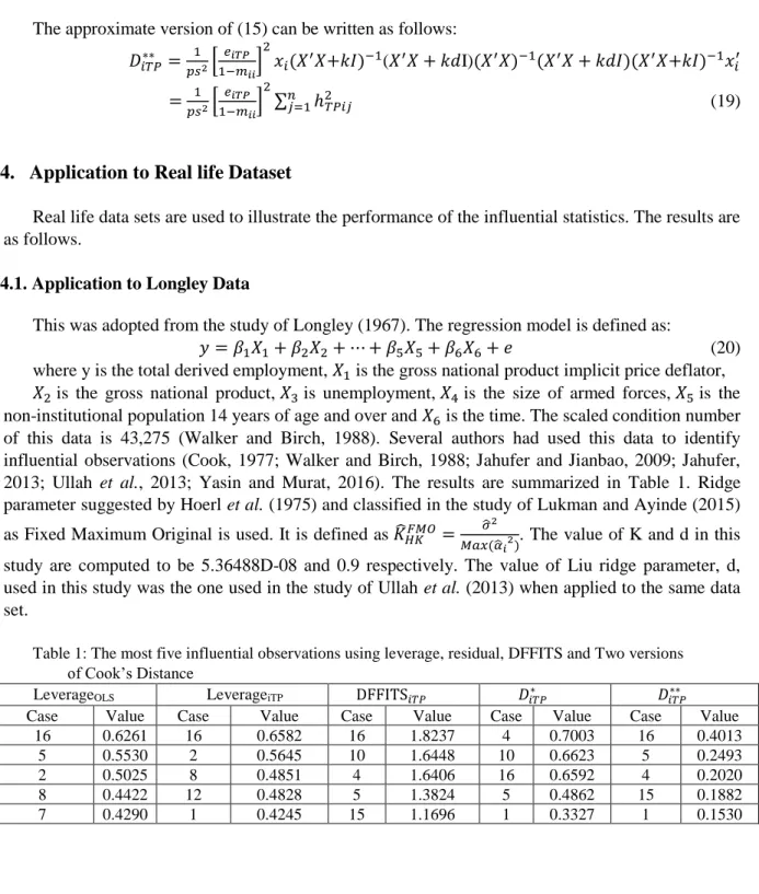
Table 1: The most five influential observations using leverage, residual, DFFITS and Two versions of Cook’s Distance
LeverageOLS LeverageiTP DFFITS𝑖𝑇𝑃 𝐷𝑖𝑇𝑃∗ 𝐷𝑖𝑇𝑃∗∗
Case Value Case Value Case Value Case Value Case Value
16 0.6261 16 0.6582 16 1.8237 4 0.7003 16 0.4013
5 0.5530 2 0.5645 10 1.6448 10 0.6623 5 0.2493
2 0.5025 8 0.4851 4 1.6406 16 0.6592 4 0.2020
8 0.4422 12 0.4828 5 1.3824 5 0.4862 15 0.1882
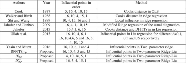
Table 2: Summary of most influential diagnostics on Longley datasets compare with propose
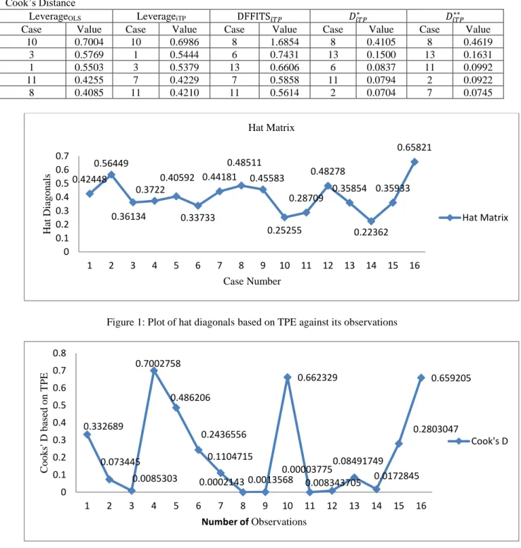
Table 1 shows that the leverage based on OLS and the proposed estimator identified observations 16, 2 and 8 as leverages in common but different in order of ranking. This also agrees with the study of Yasar and Murat (2016) where the first three leverages are case number 16, 2 and 8. This is further illustrated in Figure 1. Figure 1 is the plot of the hat diagonal matrix against the observations. The summary from to Table 2 shows that the proposed statistics DFFITSiTP identified the same value that Cook (1997) and Ullah (2013) identified as influential points, though, in a different order. DiTP* and
* * iTP
D identified the same cases as identified by other authors except case 1. The result is also validated in Figure 2.
4.2. Application to Hald Data
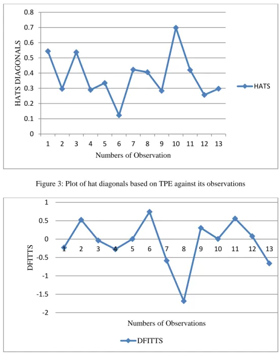
This has been previously adopted by Cook (1977); Yasin and Murat (2016) in the investigation of influential observations. Four regressors were used with thirteen (13) observations. The condition number of matrix X is computed to be 249.578 which show that the model suffers the problem of strong multicollinearity. Cook (1977) identified observations 8, 3, 11, 6 and 13 as influential points in this order. Yasin and Murat (2016) detect the influential points to be 8, 11, 10, 6 and 13 when Cooks Distance based on Two-parameter ridge was used. Observations 8, 11, 10, 3 and 6 were identified when generalized cooks D was used while observations 8, 11, 6, 10 and 13 were identified with the use of DFFITS based on Two-parameter ridge. The value of k and d in this study are computed to be 0.0076761and 1.18495 respectively. The results obtained in this study are summarized in Table 3. It was observed that the Cooks D obtained in this study and previous study performs similarly by identifying cases 8, 13, 6 and 11 in common but the order of appearance differs. DFFITS based on OLS identified cases 8, 11, 7, 2 and 4 as influential observations. The method of DFFITS suggested by Yasin and Murat (2016) identified the cases 8, 11, 6, 10 and 13 as influential while the method proposed in this study identified cases 8, 6, 13, 7 and 11 as influential points. Comparing the three methods, observation 8 is the most influential. However, the method proposed in this study and that of Yasin and Murat (2016) identifies four cases in common, though, the order differs. The new diagnostics defined based on Two-parameter Liu ridge estimator competes favorably with the existing ones.
Authors Year Influential points in
order
Method
Cook 1977 5, 16, 4, 10, 15 Cooks distance in OLS
Walker and Birch 1988 16, 10, 4, 15, 1 Cooks distance in ridge regression
Shi and Wang 1999 10, 4, 15, 16 and 1 Local influence in ridge regression
Jahufer and Jianbao 2009 16, 4, 1, 10, 15 Modified Ridge regression of the usual diagnostics
Jahufer 2013 15,4 1, 6, 16 Cooks distance and DFFITs in in Liu regression
Ullah et al. 2013 16, 10, 4, 6, 1
16, 10,4,6, 5 and 16, 5, 4, 10, 15
Influential points in Liu regression for different d=0.1, 0.5 and 0.9 respectively
Yasin and Murat 2016 16, 10, 6, 1 and 4 Influential points in Two–parameter ridge
DFFITS𝑖𝑇𝑃 Proposed 16, 10, 4, 5 and 15 Influential points in Two–parameter Ridge-Liu
𝐷𝑖𝑇𝑃∗ Proposed 4, 10, 16, 5, 1 Influential points in Two–parameter Ridge-Liu
Table 3: The most five influential observations using leverage, residual, DFFITS and Two versions of Cook’s Distance
LeverageOLS LeverageiTP DFFITS𝑖𝑇𝑃 𝐷𝑖𝑇𝑃∗ 𝐷𝑖𝑇𝑃∗∗
Case Value Case Value Case Value Case Value Case Value
10 0.7004 10 0.6986 8 1.6854 8 0.4105 8 0.4619
3 0.5769 1 0.5444 6 0.7431 13 0.1500 13 0.1631
1 0.5503 3 0.5379 13 0.6606 6 0.0837 11 0.0992
11 0.4255 7 0.4229 7 0.5858 11 0.0794 2 0.0922
8 0.4085 11 0.4210 11 0.5614 2 0.0704 7 0.0745
Figure 1: Plot of hat diagonals based on TPE against its observations
Figure 2: Plot of Cook’s D based on TPE against its observations
0.42448 0.56449 0.36134 0.3722 0.40592 0.33733 0.44181 0.48511 0.45583 0.25255 0.28709 0.48278 0.35854 0.22362 0.35933 0.65821 0 0.1 0.2 0.3 0.4 0.5 0.6 0.7 1 2 3 4 5 6 7 8 9 10 11 12 13 14 15 16 Hat Diag o n als Case Number Hat Matrix Hat Matrix 0.332689 0.073445 0.0085303 0.7002758 0.486206 0.2436556 0.1104715 0.0002143 0.0013568 0.662329 0.00003775 0.008343705 0.08491749 0.0172845 0.2803047 0.659205 0 0.1 0.2 0.3 0.4 0.5 0.6 0.7 0.8 1 2 3 4 5 6 7 8 9 10 11 12 13 14 15 16 C o o k s' D b ased o n T P E Number of Observations Cook's D
Figure 3: Plot of hat diagonals based on TPE against its observations
Figure 4: Plot of DFFITS based on TPE against its observations
5. Conclusion
The problems of multicollinearity and influential points have been jointly considered in this paper. A new diagnostic measures using Two-parameter Liu-Ridge Estimator (TPE) was proposed. The approximate case deletion formulas in TPE using Sherman-Morrison-Woodbury theorem by Rao (1973) were used to obtain the approximate versions of DFFITS, the two versions of COOK distance. The performance of these measures was illustrated with two real life dataset. The results show that the proposed measures compete favorably with the existing ones in identifying influential observations. Index plot adopted in this study is a conventional procedure to identified influential cases, even though, no conventional cut off points are introduced or developed for the TPE influence diagnostics. These measures will assist practitioners to decide whether to retain, remove or down sized influential points using robust estimators when identified in a study.
0 0.1 0.2 0.3 0.4 0.5 0.6 0.7 0.8 1 2 3 4 5 6 7 8 9 10 11 12 13 HA T S DI A GONA L S Numbers of Observation HATS -2 -1.5 -1 -0.5 0 0.5 1 1 2 3 4 5 6 7 8 9 10 11 12 13 DFI T T S Numbers of Observations DFITTS
References
[1] Belsley, D. A., Kuh, E. and Welsch, R.E. (1980). Regression Diagnostics; Identifying Influence Data and Source of Collinearity. Wiley, New York.
[2] Belsley, D.A. (1991). Conditioning Diagnostics: Collinearity and Weak Data in Regression. NewYork: Wiley.
[3] Cook, R.D. (1977) Detection of influential observations in linear regression. Technometrics 19: 15-18.
[4] Cook, R. D. (1982) and Weisberg, S. (1980). Characterization of an empirical influence function for detecting influential cases in regression. Technometrics, 22, 495-508.
[5] Cook, R. D. (1982) and Weisberg, S. (1982). Residuals and Influence in Regression. Chapman and Hall, New York.
[6] Cook, R. D. (1986). Assessment of local influence (with discussion). Journal of Royal StatisticalSociety, B. 48, 133-69.
[7] Chatterjee, S., Hadi, A. S. (1986). Influential observations, high leverage points, and outliers inlinear regression. Statistical Science, 1, 379-416.
[8] Draper, N.R. and John, J.A. (1981). Influential observations and outliers in regression. Technometrics, 23, 21-26.
[9] Hoerl, A.E. and Kennard, R.W. (1970). Ridge regression: biased estimation for non-orthogonal problems. Technometrics, 12, 55-67.
[10] Hoerl, A. E., Kennard, R. W. and Baldwin, K. F. (1975). Ridge regression: Some simulation. Communications in Statistics, 4 (2), 105–123.
[11] Jahufer, A., and Jianbao, C. (2009). Assessing global influential observations in modified ridge regression. Statistics & Probability Letters, 79(4), 513-518.
[12] Jahufer, A. and Chen, J. (2008). Identifying Local Influence in Modified Ridge Regression Using Cook’s Method. Sri Lankan Journal of Applied Statistics, 9, 93-108.
[13] Jahufer, A. (2013). Detecting Global Influential Observations in Liu Regression Model. Open Journal of Statistics, 3(1), 5-11.
[14] Johnston, J. (1972). Econometric Methods, 2nd Ed. McGraw-Hill Book Co., Inc., New York. [15] Liu, K. (1993). A new class of biased estimate in linear regression. Communications in Statistics,
22(2), 393-402.
[16] Longley, J.W. (1967) An appraisal of least squares programs for electronic computer from the point of view of the user. Journal of American Statistical Association 62: 819-841.
[17] Lukman, A. F. and Ayinde, K. (2015). Review and classification of the Ridge Parameter Estimation Techniques. Hacettepe Journal of Mathematics and Statistics. Accepted for Publication.
[18] Mandel, J. (1982). Use of the singular value decomposition in regression analysis. The American Statistician, 36(1), 15-24.
[19] Ozkale, M. R. and Kaciranlar, S., (2007). The restricted and unrestricted two-parameter estimators. Commun. Statist. Theor. Meth. 36, 2707–2725.
[20] Rao, C. R. (1973). Linear statistical inference and its applications, 22: John Wiley & Sons. [21] Shi, L. (1997). Local influence in principal components analysis. Biometrika, 84(1), 175-186. [22] Shi, L., and Wang, X. (1999). Local influence in ridge regression. Computational Statistics and Data
Analysis, 31(3), 341-353.
[23] Ullah, M. A., Pasha, G. R., and Aslam, M. (2013). Assessing Influence on the Liu Estimates in Linear Regression Models. Communications in Statistics - Theory and Methods, 42(17), 3100-3116. [24] Yasin, A. and Murat, E. (2016). Influence Diagnostics in Two-Parameter Ridge Regression. Journal
of Data Science, 14, 33-52.
[25] Walker, E. and Birch, J. B. (1988). Influence Measures in Ridge Regression. Technometrics, 30(2), 221- 227.