A Study of Bayesian Estimation and Comparison of Response Time Models in Item Response Theory

A Study of Bayesian Estimation and Comparison of Response Time

Models in Item Response Theory

By

Hongwook Suh

Submitted to the graduate degree program in the

Department of Psychology and Research in Education

and the Graduate Faculty of the University of Kansas

in partial fulfillment of the requirements for the degree of

Doctor of Philosophy.

The Dissertation Committee for Hongwook Suh certifies

that this is the approved version of the following dissertation:

A Study of Bayesian Estimation and Comparison of Response Time

Models in Item Response Theory

_______________________ Chairperson

Abstract

Response time has been regarded as an important source for investigating the relationship between human performance and response speed. It is important to examine the relationship between response time and item characteristics, especially in the perspective of the relationship between response time and various factors that affect examinee’s responses. The purpose of this study was to examine different scoring models using response time data in conjunction with item response models. In this study distinctive response time models incorporated in IRT were compared, and the relationship between item characteristics and examinee ability as well as response time were examined using real and simulated data.

Bayesian estimation using Markov Chain Monte Carlo (MCMC) methods for Thissen’s (1983) lognormal response time model, Wang and Hanson’s (2005) 4PL RT model, and van der Linden’s (2007) hierarchical framework were applied to the investigation of response time on real data. Overall, van der Linden’s (2007) hierarchical framework showed the most reasonable outcomes from the real data analysis when it was compared with the 4PL RT and Thissen’s models. Compared with Wang and Hanson’s (2005) 4PL RT model in the simulated data analysis, the hierarchical framework also showed better results as follows: (1) better recoveries in item and examinee parameter, (2) reasonable explanations in delineating relationships between response time and other related parameters in the model. There were no clear relationships among speed-related parameters across the models when the relationships between the response time-related parameters were investigated across the response time models. This was due to the different definitions and different parameterization procedures of the speed-related parameters based on the response time model.

Acknowledgement

I am grateful to all the people that I met while I have prepared this dissertation. My greatest debt is to Dr. William Skorupski, my academic advisor. He is the one who brought me to the field and provided me unfailing effort and knowledge to pursue this project as my dissertation. I also want to thank each member of my dissertation committee: Dr. Bruce Frey, Dr. Neal Kingston, Dr. Vicky Peyton, and Dr. Kris Preacher. Especially, I would like to thank Kris, who read my writing and corrected every single word. I also want to thank Dr. Kingston, who provided me a financial aid for the last semester at KU. I am also indebted to Bruce and Vicky for their heartful encouragement throughout my study for the last years.

Without the support and cooperation of my family, it would hardly be possible to finish this dissertation. I would like to thank my wife, Sunhyoung Lee, for her loving encouragement and enduring support every day. I also thank my son and daughter, Elliott and Elaine, and my to-be-born daughter for giving me plentiful good reasons to finish dissertation. I also would like to express deep gratitude to my parents and parents-in-law, who supported and encouraged me in their prayers every day since I began to study in the United States.

Table of Contents

Abstract ... iii

Acknowledgement ... iv

List of tables ...viii

List of figures ... ix List of equations ... x List of appendices ... xi Chapter 1. Introduction ... 1 Statement of problem ... 1 Purpose ... 4 Research questions ... 5 Hypotheses ... 6

Chapter 2. Literature review ... 8

Power and speed test ... 9

Historical perspectives on response time anlaysis ... 9

Item response theory ... 11

Response time analysis and computerized tests ... 13

Speededness ... 13

Computer adaptive testing (CAT) ... 15

Relationships between response time and ability ... 16

Scoring models using response time ... 18

Thissen’s (1983) model ... 19

4PL response time model ... 21

Hierarchical framework ... 22

Bayesian estimation in IRT ... 24

Markov Chain Monte Carlo (MCMC) method ... 27

Gibbs sampler ... 29

Checking model convergence ... 30

Chapter 3. Methods ... 34

Study 1 ... 34

Data ... 34

Estimation methods ... 35

Checking model convergence and DIC ... 38

Study 2 ... 39 Data generation ... 39 Factors of investigation ... 40 Measured criteria ... 40 Chapter 4. Results ... 42 Study 1 results ... 42

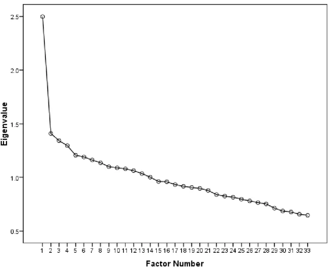
Preliminary data analysis ... 42

Response time models implementation ... 49

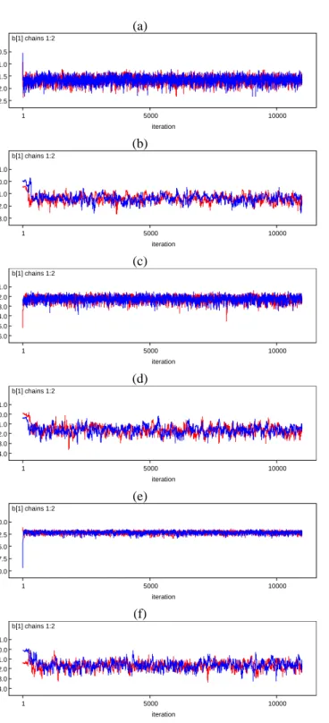
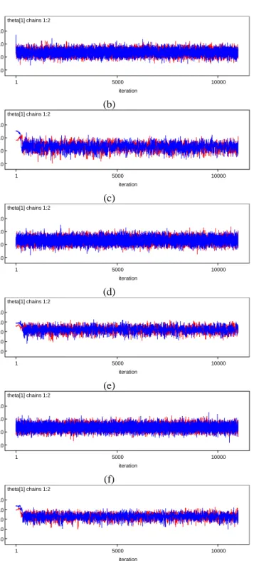
Convergence check ... 49

Model goodness of fit and comparison ... 53

Comparison of parameter estimates ... 53

Comparison of response time related parameter estimates ... 56

Study 2 results ... 60

DIC comparison ... 60

Parameter recovery analysis ... 62

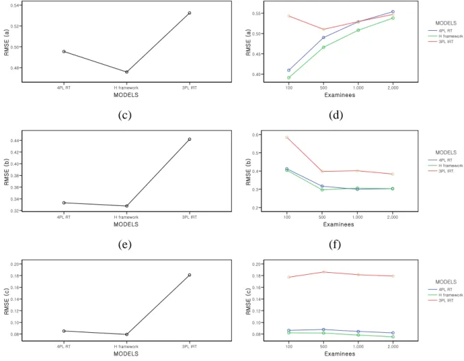
Item parameter recovery ... 62

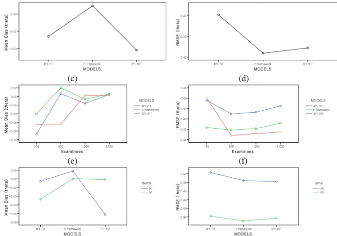
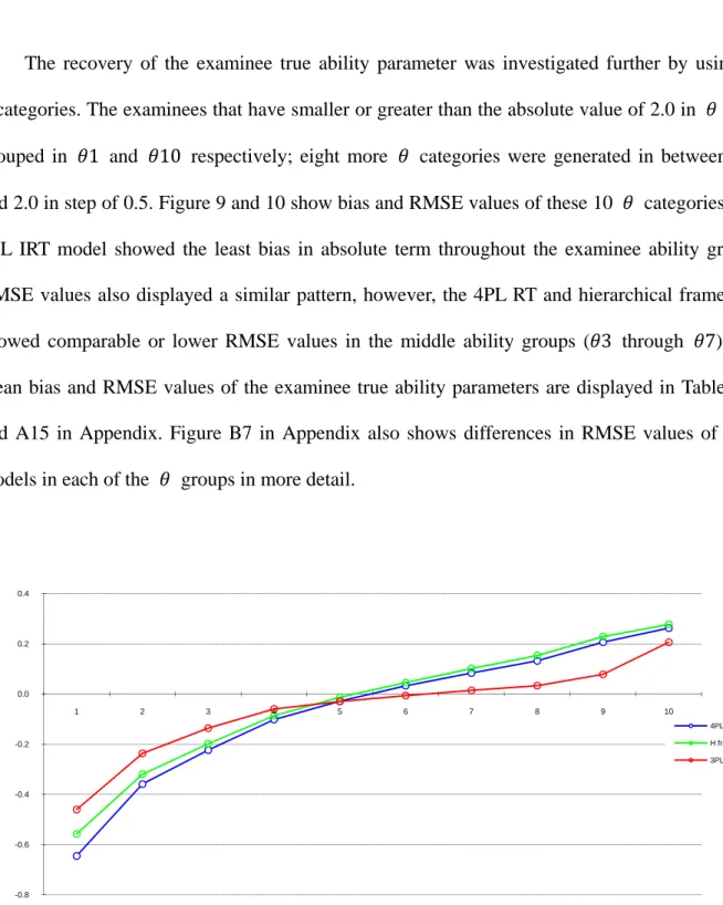
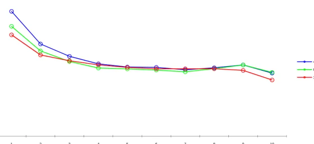
Examinee true ability parameter recovery ... 69

Correlations between item parameters and estimates ... 78

Correlation between examinee parameters and estimates ... 81

Correlation between response time related parameters and estimates ... 83

Chapter 5. Discussion ... 87

Model comparison in the real data study ... 88

Overall results of analysis ... 88

Response time-related parameter estimation ... 89

Model comparison in the simulated data study ... 90

Overall results of analysis ... 90

Correlation between response time-related parameters ... 94

Relationship between response time models ... 95

Limitations of the study and further research questions ... 97

Conclusion ... 98

List of Tables

Table 1. Descriptive statistics for responses and response times ... 43

Table 2. Frequencies for missing responses and response times ... 43

Table 3. Means and standard deviations for item parameter estimates from the CTT and IRT ... 44

Table 4. Item-total score correlation coefficients and reliability indices ... 46

Table 5. Item parameter estimates from the CTT and IRT models ... 47

Table 6. Descriptive statistics for item responses times ... 48

Table 7. DIC values from the responses time models ... 53

Table 8. Means and standard deviations for the item and examinee parameter estimates from the response time models ... 54

Table 9. Correlations between the item difficulty parameter estimates among the models ... 55

Table 10. Correlations between the examinee true ability parameter estimates among the models ... 55

Table 11. Descriptive Correlations between the item difficulty and item speed parameter estimates (N=33); correlations between the examinee true ability and speed parameter estimates (N=975) ... 58

Table 12. Correlations among the item parameters and mean response time (N=33); correlations among the examinee parameters and response time (N=975) ... 59

Table 13. DIC values for the 4PL RT model and hierarchical framework ... 61

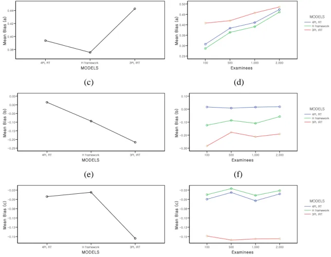
Table 14. Mean bias for the item parameters in the 3 models ... 63

Table 15. Mean RMSE for the item parameters in the 3 models ... 65

Table 16. Relative efficiency for the item parameters in the 3 models ... 67

Table 17. The MANOVA results for the bias of the item parameters ... 68

Table 18. The post hoc comparison results for the bias of the item parameters ... 68

Table 19. The MANOVA results for the RMSE of the item parameters ... 69

Table 20. The post hoc comparison results for the RMSE of the item parameters ... 69

Table 21. Bias and RMSE for the examinee true ability parameter in the 3 models ... 70

Table 22. Relative efficiency for the examinee true ability parameter in the 3 models ... 72

Table 23. The MANOVA results for the measured criteria of the examinee true ability ... 73

Table 24. The post hoc comparison results for the measured criteria of the examinee true ability ... 73

Table 25. The MANOVA results for the RMSE of the examinee ability based on the ability groups ... 76

Table 26. The post hoc comparison results for the RMSE of the examinee true ability based on ability groups ... 77

Table 27. Correlation between the item parameters and estimates in the 3 models ... 78

Table 28. Correlation between the examinees true ability parameter and estimates in the 3 models ... 81

Table 29. Correlations between item and examinee parameter estimates from the 2 response time models ... 83

Table 30. Correlations between responses time-related parameter estimates from the 2 response time models ... 85

List of Figures

Figure 1. The hierarchical framework for modeling speed and accuracy on items ... 22

Figure 2. Histograms of total score and total response times ... 43

Figure 3. Scree plot of eigenvalues from factor analysis ... 45

Figure 4. Some representative history plots of the item difficulty parameter estimates ... 51

Figure 5. Some representative history plots of the examinee true ability parameter estimates ... 52

Figure 6. Mean bias for the item parameters in the 3 models ... 64

Figure 7. Mean RMSE for the item parameters in the 3 models ... 66

Figure 8. Bias and RMSE for the examinee true ability parameter in the 3 models ... 71

Figure 9. Bias for the examinee true ability parameter based on the examinee ability groups ... 74

Figure 10. RMSE for the examinee true ability parameter based on the examinee ability groups ... 75

Figure 11. Correlation between item parameters and estimates in the 3 models ... 79

Figure 12. Correlation between item parameters and estimates in the 2 response time models ... 80

Figure 13. Correlation between the examinee true ability parameters and estimates in the 3 models; Correlation between the examinee true ability parameters and estimates in the 2 response time models ... 82

Figure 14. Correlation between the item speed and item difficulty parameters; correlation between the examinee speed and examinee ability parameters; correlation between the response time discrimination and item discrimination parameters ... 86

List of Equations

Equation 1. 3PL IRT model ... 12

Equation 2. Thissen’s lognormal response time model ... 19

Equation 3. Thissen’s lognormal response time model (a 3PL application) ... 20

Equation 4. 4PL response time (RT) model ... 21

Equation 5. 3PL IRT model in the hierarchical framework ... 23

Equation 6. Lognormal response time model in the hierarchical framework ... 23

Equation 7. Bayes’ theorem ... 25

Equation 8. Marginal probability in Bayes’ theorem ... 25

Equation 9. Bayes’ theorem in terms of a probability density function ... 25

Equation 10. Posterior density in Bayes’ theorem ... 26

Equation 11. Joint distribution of a 3PL IRT model ... 26

Equation 12. DIC calculation ... 33

Equation 13. Bias calculation ... 41

Equation 14. RMSE calculation ... 41

List of Appendices

Appendix A ... 107

Chapter 1. Introduction

Statement of Problem

Response time on items in a computer–based test enables researchers to study examinees’ responses further in test settings and provides valuable information. Response time data allow understanding of examinee behavior from data–based perspectives not previously feasible, and illustrate the important role that these investigations can play in test development, administration, and validation (Schnipke & Scrams, 2002; Zenisky & Baldwin, 2006). Response time has been one of many popular topics in traditional psychological measurement, investigating the relationship between human performance and response speed. Although using response time data is not fully developed in the educational measurement field, it is valuable in understanding human behavior in test settings. It is important to examine the relationship between response time and item characteristics, especially in the perspective of the relationship between response time and various factors that affect examinees’ responses.

Response time and test performance have been studied in various ways. Schnipke and Scrams (2002) enumerated the related areas in the measurement field such as scoring models using response time data in conjunction with response data, speed–accuracy relationships, strategy usage, speededness, pacing, predicting finishing times and setting time limits, and subgroup differences. Because several areas are interrelated and quite different perspectives exist depending on the situation, it is not easy to consider only one area without considering the rest. For example, Gulliksen (1950) pointed out two factors of the tests and contrasted power and speed tests. In traditional psychological measurement, response speed and accuracy have been regarded as

interchangeable concepts as accepted in the speed test. However, in the power test situation, speed theoretically is not a related concept; accuracy is independent from response speed. Likewise, speed–accuracy (speed–ability) trade–off and scoring models using response time data also have quite different perspectives when they are applied to speed tests from when they are applied to the power test situation.

Most major standardized achievement tests are power tests, which indicate the goal of testing is to measure how accurately examinees respond to the item rather than how quickly they finish the item. In reality, most tests contain both speed and power components, requiring an assessment of speededness (Rindler, 1979). However, the amount of speededness in operational testing has been underestimated prior to the research on speededness using response time in computer–based testing (Oshima, 1994; Schnipke, 1995; Schnipke & Scrams, 1996). Most tests have multiple choice items, no penalty for incorrectly responded items, and restricted time limits. Therefore, rapid guessing behavior, especially at the end of testing, may be easily attempted by the examinees. The effects of speededness and rapid guessing behavior are highly evident in terms of measurement accuracy. Undetected speededness affects erroneously estimation procedures of item characteristic parameters and examinee true ability parameter (Oshima, 1994). Various research studies have been conducted on speededness by investigating aberrant behaviors (e.g., Schinipke, 1995), strategy usage (e.g., Bontempo & Julian, 1997; Gitomer, Curtis, Glaser, & Lensky, 1987), estimating optimal time to solve the items (e.g., Bridgeman & Cline, 2004), and moderated effort (e.g., Wise & DeMars, 2006). Although each study has indicated a different approach in terms of its focus and design, these studies all contribute to the construction of a nomological validity network for the effect of response time in computer–based testing (Cronbach & Meehl, 1955;

Messick, 1981).

The most commonly observed examinee behavior in testing is accuracy on test items. Although it is not always directly reflected, the score, an examinee receives on the test, is based on their accuracy. Likewise, most psychometric research has focused on scores in some form (Schnipke & Scrams, 2002). Given the primary interest in test scores and the possible effect of speededness, researchers have tried to develop models that use response time in the scoring process (e.g., Roskam, 1987, 1997; Thissen, 1983; van der Linden, 2007; Verhelst, Verstralen, & Jansen, 1997; Wang & Hanson, 2005). Several models have been proposed differing in terms of the assumed response time distributions, the assumed relationship between ability and response speed, and the nature of items for which the model was designed. van der Linden (2006) categorized these models under two distinct approaches: modeling response time in the framework of an item response theory (IRT) and separate models for response time and response for the item. He also stated that, for the educational assessment field, it is pertinent to adopt a response time model integrated in the framework of IRT.

Thissen’s model (1983) is one of the oldest models using response time, and has a lognormal distribution of the response time on an item with a two–parameter logistic (2PL) IRT structure. This model has person speed and item speed parameters with a time interpretation. The 2PL IRT response component is regressed on the response time and indicates two sources of relationships: (a) response time and examinee ability, (b) response time and item difficulty. Similarly, Wang and Hanson (2005) proposed the 4PL IRT response time model, which has an examinee and an item slowness parameter in the typical 3PL IRT model. Those two models tried to reflect two different components of examinee data from testing settings. In addition, van der

Linden (2007) proposed a hierarchical modeling framework consistent with the previous two traditions. This model has two separate response and response time models as first level models and the integrated model of their parameters as a second level. Therefore it can be possible to estimate response time and response models independently at the first level as well as identify the relationships between two separate models. More specifically, this hierarchical framework can distinguish the following levels: (1) the within–person level, at which the value of the person parameters are allowed to change over time (e.g., due to a change of strategy or external conditions); (2) the fixed–person level, at which the parameters remain constant; and (3) the level of a population of fixed persons, for which there is a distribution of parameter values across persons (van der Linden, 2007). van der Linden’s (2007) hierarchical framework enables one to locate the sources of variability between examinee ability and response time as well as item characteristics and response speed.

Purpose

The purpose of this study is to compare two different scoring models using response time data in conjunction with item response models. Various scoring models incorporating response time have been proposed. However, there are not many studies comparing different orientations on the response time and item response model. Most of the studies using response time models have been focused on model fit to the given data. Although it is not easy to compare models which are founded on different theoretical bases, it is worthwhile considering the potential benefits of using response time information in educational assessment. The results from the analysis of response time allow us to devise appropriate scoring models, secure test validity under the threats of various

factors affecting the assumptions of unidimensional IRT, and further examine human behavior in various test settings.

In this study distinctive response time models incorporated in IRT were compared, and the relationship between item characteristics and examinee ability as well as response time were examined using real and simulated data. Bayesian estimation using Markov Chain Monte Carlo (MCMC) methods for Thissen’s (Thissen, 1983) lognormal response time model, Wang and Hanson’s (Wang & Hanson, 2005) 4PL RT model, and van der Linden’s (van der Linden, 2007) hierarchical framework were applied to the investigation of response time on real data. After the application of those response time models on real data, examinee ability and item characteristic parameters from the item response models, as well as speed–related parameters from response time models, were estimated and used for generating simulated data. Those models were, then, applied to simulated data and compared under various conditions of testing situations by utilizing Bayesian posterior estimates.

Research Questions

The research questions addressed in this study are as follows:

1. Among the 4PL response time (RT), hierarchical framework, and Thissen’s model, which is the best method for scoring examinees’ item responses when response time data are available on real data?

2. What are the relationships between the response time–related parameters (examinee and item slowness, time intensity and time discrimination parameters) from different models that explain the speed–accuracy trade–off among item characteristics and examinee ability in item responses?

3. Between the 4PL RT model and hierarchical framework, which model is better to use for scoring examinees’ responses with response time data under different conditions such as various numbers of examinees, different number of items, and different relationship among item characteristics and examinee ability?

Hypotheses

The 4PL RT model and the hierarchical framework showed successful results in applications to real data as well as simulated ones (e.g., Wang & Hanson, 2005; van der Linden, 2007; Fox, Klein Entink, & van der Linden, 2007). However, Wang & Hanson’s (2005) 4PL RT model has several limitations when applied in real situations. Because the 4PL RT model has an assumption of independence between response time and the examinee ability parameters, it is unrealistic in most timed testing environment. Later, Wang (2006) modeled the joint distribution of response time using a 1PL Weibull distribution to extend the 4PL RT model. The joint distribution of a response and response time model enables to remove the independence assumption which the 4PL RT model has; however, it did not show much improvement from the typical IRT models that do not consider response time.

It was hypothesized that van der Linden’s (2007) hierarchical framework would fit the data better when there is a positive or negative relationship between item characteristics and examinee’s ability parameters. As item difficulty increases, it is assumed that it will take longer for examinees to finish such items than easier ones. Likewise, it is also assumed that high level examinees will complete problem solving processes faster than their low level counterparts. The hierarchical framework allows researchers to estimate item and examinee parameters separately by

distinguishing different models of examinee response time and responses. Thus, identifying various sources of response time latency is available by using the hierarchical framework on response time data. However, it is also assumed that the complex models do not always produce better results than simpler ones do. The principle of parsimony is one of the factors that should be considered when making decisions about model fit and model comparison.

Chapter 2. Literature review

More tests are now being administered on computers, providing easy collection of response times in standard, operational testing settings. As response times are becoming more available, it is more prevalent to make use of this information. Many studies have been done in the area of scoring and parameter estimation procedures utilizing response time data in conjunction with response data (e.g., Roskam, 1987, 1997; Thissen, 1983; van der Linden, 2007; Verhelst, Verstralen, & Jansen, 1997; Wang & Hanson, 2005). This chapter presents a summary of the relevant studies on speed, accuracy, and performance in computer–based tests. It begins with some prerequisite definitions of related concepts, including item response theory, preceding discussions on the relationship of speed and accuracy. Various studies investigating the relationships between ability and speed will be summarized and scoring models with response time data will follow. Finally, for the model parameter estimation procedures, Markov Chain Monte Carlo (MCMC) methods using Gibbs sampling will be introduced.

Power and speed tests

Gulliksen (1950) pointed out two essential factors for the tests: speed and power. A pure power test has items with a range of difficulties and an infinite time limit. The goal of a pure power test is to measure how accurately examinees respond to the items. Because power tests have a time limit long enough to permit everyone to attempt all items, item difficulty is steeply graded and includes items too difficult for anyone to solve, so it is hard to get a perfect score. On the other hand, the goal of a pure speed test is to measure how quickly examinees respond to the items. A test is constructed with easier items and a time limit is so short that no one can finish all the items. On pure speed testing, each person’s score directly reflects the speed with which each examinee worked. Anastasi (1976) also defines that a speed test is when the speed of performance determines individual differences. However, both power and speed tests are designed to prevent the achievement of perfect scores.

Historical perspectives on response time analysis

As indicated by Gulliksen’s (1950) definitions of power and speed tests, it is generally accepted that there exists interchangeability between speed and ability. Because measuring the time it takes an examinee to process information is deemed indicative of how examinee processed it, researchers had believed speed and accuracy measured the same construct. Spearman (1927) became one of the earliest proponents of the theory that the speed at which an examinee completed a test and the accuracy from the results gave equivalent information. Thus he argued that an examinee’s mental ability could be measured on a scale of accuracy, a scale of speed, or some combination of the two constructs (Spearman, 1927). However, the study of these two

constructs on complex tasks did not show that they were same constructs by subsequent researchers (Baxter, 1941; Bridges, 1985; Foos, 1989). Myers (1952) demonstrated that speed and accuracy comprised orthogonal factors in test scores, indicating that an examinee’s speed in testing is not related to the examinee’s ability. Various other studies also confirmed that Spearman’s (1927) interchangeability concept on speed and ability is unrealistic in educational assessment settings (Schnipke & Scrams, 2002).

The speed–accuracy trade–off is one of best known findings in response time research (Luce, 1986). The speed–accuracy trade–off implies that if a person chooses to perform a task at a higher speed rather than a relatively lower speed, their level of accuracy will become lower. It is obvious that the trade–off can be applied either to pure speed tests or pure power tests. However, studies on response time for correct and incorrect responses showed different directions. Bergstrom, Gershon, and Lunz (1994) found that examinees spent more time on items they answered incorrectly than on items they answered correctly. Hornke (2000) also found that relatively longer response times are required to respond to questions that are answered incorrectly. A variety of systematic studies on item response times in computerized adaptive testing found that incorrect answers require much longer processing time than correct answers (Rammsayer, 2004).

It is argued that most wrong responses are from the lower ability group, examinee’s lower ability used to relate to relatively longer response time in the marginal analysis (Bergstrom et al., 1994; Hornke, 2000). As explained by Simpson’s paradox (Agresti, 2002; Simpson, 1951), taking the ability of examinees into account would result in explaining a somewhat different relationship between response time and response accuracy. Therefore, the relationship among response speed and related examinee characteristics needs to be verified by further examining the relationship

among examinees’ ability, item difficulties, and response time simultaneously.

It is reasonable to assume that the relationships between accuracy and speed are not to be correlated without considering other effects derived from item and examinee characteristics. Schnipke and Scrams (2002) pointed out that a great deal of previous research has used confounding measures to investigate the relationship of speed and accuracy. Specifically, examinee speed is easily confounded with item difficulty when it is administered on computer adaptive tests (CAT). More discussion of the relationships between accuracy and speed, ability and response time will be presented in the following sections.

Item response theory

Item response theory (IRT) is a statistical theory about the probability of an examinee responding to an item correctly at a given level of latent proficiency. IRT models specify how test items and examinee responses relate to the abilities of the examinees that are measured by the items in the test (Hambleton & Jones, 1993). Two basic assumptions are required to use these IRT models (Hambleton & Jones, 1993; Hambleton, Swaminathan, & Rogers, 1991). First, a unidimensionality assumption is required, meaning that there is one construct of a given test. The items in a test are considered to be unidimensional when a single factor or trait accounts for a substantial portion of the total test score variance. It is a broad concept which also encompasses local independence and parameter invariance assumptions; item responses are deemed locally independent when examinees’ ability is the sole source that affects responses on the items. Second, the item characteristic function or curve (ICC) is needed to form a mathematical representation. It delineates the relationship between examinees’ unobserved latent ability and observed test scores

from responses to the items (Hambleton & Jones, 1993; Swygert, 1998).

Many models have been formulated within the general IRT framework; however, usually one, two, or three parameter logistic functions will be considered when the model is applied to dichotomously scored items. In terms of dichotomously scored test items, on which responses are designated either correct or incorrect, all IRT models express the probability of a correct response to a test item as a function of

θ

where Pij(

θ

θ

which has generally scaled with a mean of 0 and standard deviation of 1. bj is the item difficulty or

location parameter, aj is the discrimination or slope parameter, which is bounded by 0, and

generally ≤ 2.0. cj is the pseudo guessing or lower asymptote parameter. This is bounded by 0 and

1, and generally ≤ 0.25 depending on the number of alternative answers in the items. Under the typical IRT framework, both the test items and the examinees responding to the items are arrayed on

θ

θ

θ

referred to as the person’s ability or proficiency. The position of item j on

θ

is termed the item’s difficulty. It is expected that the probability of a correct response to item j will increase monotonically as (

θ

constrained forms of the typical 3PL model; the item discrimination parameter is set to 1.0 in the 1PL IRT model; the pseudo guessing parameter is set to zero in the 1PL and 2PL models.

Response time analysis and computerized tests

The availability of item response times, made possible by computerized testing, provides an entirely new type of information about items. Previously, only total testing time and item responses were available. However, in addition to knowing the accuracy with which test takers answer an item, it is now possible to investigate the amount of time examinees spend on each item. This allows one to examine the relationships among examinee ability, item characteristics, and response speed (Schnipke & Scrams, 1999). Various other kinds of information in test settings can be obtained from response time data, such as speededness, pacing, strategies used, and time limit.

Speededness

Speededness is the effect of time limits on the candidate’s scores. It is the extent to which a test is affected by time limits, which is measured when the examinee’s total incorrect score is equal to the number of items that were not attempted by the examinee (Evans & Reilly, 1972). Bejar (1985) stated that “a test is speeded when some portion of the test–taking population does not have sufficient time to attempt every itemin thetestwithin the allocatedtime.” Bontempo and Julian (1997) also defined speededness as “the degree to which the amount of time allowed for test administration affects the rate at which examinees answer items.”

Speededness is a closely related concept with other response time related constructs such as pacing, strategy use, and predicting finishing times or setting up time limits. Test speededness is gauged from the perspective of testing environment, while pacing and guessing behaviors are construed from the examinee perspectives. Likewise, strategy use in testing is also related to pacing and test speededness. Schnipke (1995) defined two distinct types of behavior when test

speededness exists: problem solving and rapid guessing behaviors. Just as rapid guessing behavior at the end of a test substantially affects the examinee’s ability estimate, test taking strategies, test wiseness, and pacing also need to be examined in the perspective of these two types of test taking behavior.

In reality, most tests contain both speed and power components, requiring assessments of certain amount of speededness (Rindler, 1979). It is argued, therefore, that a test is investigated the degree of speededness instead of existence of speededness or lack thereof (Lu & Sireci, 2007). It is obvious that that the amount of speededness in testing has been underestimated until recent research on speededness conducted using response time in computerized tests (Schnipke & Scrams, 2002). Schaeffer, Reese, Steffen, McKinley, and Mills (1993) examined the average item response time from the Graduate Record Examination (GRE) and concluded that the time limits were sufficient. On the other hand, Bridgeman (2004) found that an examinee who worked at the mean rate for the first 20 items would require 11 more minutes than what was allowed on the GRE.

Speededness in a computerized testing environment has raised significant validity issues in some studies. Oshima (1994) demonstrated that undetected speededness can cause a significant problem on many large–scale standardized tests such as TOEFL and SAT (e.g., Angoff, 1989; Bejar, 1985; Schmidt & Dorans, 1990). Bridgeman (2000) states that time limits may raise equity issues if the limit is imposed for administrative convenience rather than an essential part of what the test is measuring. Bridgeman, Cline, and Hessinger (2003) also concluded that the variation among examinees in the rate of response to test items constitutes an irrelevant source of difficulty in test performance. Irrespective of the definition and directions of the research studies, all research in speededness ended up with one agreement of detrimental results of the validity of

interpretations of test scores (Lu & Sireci, 2007). As indicated by Messick (1981), it is obvious that construct irrelevant variance resulting from test speededness contributes to unreliability and invalidity of test.

Computer adaptive testing (CAT)

Computer adaptive testing (CAT) introduces new dimensions to the speededness issue. Usually, computer–based tests (CBT) implement the same administration and scoring algorithms as typical paper and pencil versions. On the other hand, a CAT modifies the difficulty of a test based on an examinee’s responses as a function of the current estimate of ability. However, these procedures may add to the cognitive load of the higher ability examinees, because more difficult items usually demand more time to solve.

Speededness in CAT is connected to the fairness issue because omitting items is no longer an option in CAT. Many studies have demonstrated that item difficulty and response time are positively correlated in CAT (Bergstrom et al., 1994; Bridgeman & Cline, 2004; Chang, 2006; Plake, 1999; Smith, 2000). This is because response time and item difficulty are closely related to critical reasoning and problem solving procedures that increase the number of steps required to answer a problem correctly. The assumption is that successive items become more difficult, it also adds more cognitive load and finally results in spending extra time to solve the item.

Various studies have consistently found that pacing and test taking strategies are also affected by speededness in CAT. Bergstrom et al. (1994) and Bridgeman and Cline (2004) concluded that it took longer for higher ability students to finish the test than lower ability students, because higher ability students are administered more difficult items. Chang (2006) also suggested

the same result, indicating the test becomes more speeded for higher ability students regardless of item types. Specifically, it is noted that higher ability examinees spend much more time on pretest items. This introduces an important piece of information to explain the relationship between ability and speededness in CAT. Because pretest items are not tailored to the examinees based on their relative ability levels, it may be generalized that more able examinees spend more time on all items regardless of whether their responses are right or wrong. Test taking strategies are also confounded by the fact that most CAT implementations prevent the test taker from reviewing previous answers, as well as from omitting answers. Bridgeman and Cline (2004) noted that more rapid guessing behavior is required for the higher ability examinees because they have more time consuming items. Bergstrom et al. (1994) also concluded that the ability and item positions are significant factors in predicting the finishing time of examinees in a within subject model. They suggested that controllable factors such as using figures, item length, and position of keyed correct answers contribute to explaining the variance of response time (Bergstrom et al., 1994).

Relationships between response time and ability

As discussed in the previous section, understanding the relationship between response time and accuracy is important in building appropriate and reasonable models. Results from previous studies indicated that there are distinct patterns among item characteristics, examinee ability, and response time. When items become more difficult, it takes more time for examinees to process (e.g., Bergstrom et al., 1994; Bridgeman & Cline, 2004; Chang, 2006; Plake, 1999; Smith, 2000). Incorrect responses take more time than correct responses (e.g., Bergstrom et al., 1994; Hornke, 2000; Rammsayer, 2004). More able examinees generally take more time to finish items than less

able examinees (e.g., Bergstrom et al., 1994; Bridgeman & Cline, 2004; Chang, 2006; Swygert, 1998). However, there are not many studies regarding systematic explanations of why such relationships exist among these factors.

The relationship between response time and examinee ability is manifested by how those components are modeled in the scoring framework. Various studies have implemented models of response time and item responses based on a range of different scoring methods and response time distributions (Schnipke & Scrams, 2002). Researchers have tried to find models that can be fit with statistical distribution functions with known properties. Normal and lognormal distribution were tested by Thissen (1983), gamma and Weibull distribution have been tested by Tatsuoka and Tatsuoka (1980) and Roskam (1997). These distributions were fit to empirical distribution functions from a computer–based test. Schnipke and Scrams (1997, 2002) found that response time data were best fit by the lognormal distribution for both exploratory and confirmatory samples and provided meaningful interpretations of the data.

van der Linden (2006, 2009) categorized existing response time models into two distinct groups based on the approaches those models have. The first one models response times in the framework of an item response theory (IRT) model. Because response times are modeled in the framework of an IRT model, it is assumed that an interaction exists between the parameters that govern the distributions of the person’s response times and response variables for the items. As discussed previously, it is often suggested that more difficult items require more time to be solved. It is also noted that this modeling is based on the speed–accuracy trade–off that has been the focus of much of the psychological literature on response times (Luce, 1983; van der Linden, 2006).

models without parametric relationships between response time and the examinee’s responses. In this approach, response time distributions are modeled without any parametric consideration of the response variables on the items, in other words, they are assumed to be independent. It is also assumed that speed is not related to the accuracy of an examinee’s responses based on an examinee’s ability. Results from some of the studies introduced in the previous section suggest this approach is feasible (e.g., Bergstrom et al., 1994; Bridgeman & Cline, 2004; Chang, 2006; Swygert, 1998). Positive as well as no relationships between response time and accuracy have been found in many studies (e.g., Bergstrom et al., 1994; Scrams & Schnipke, 1997; Swygert, 1998; Thissen, 1983).

Schnipke and Scrams (2002) pointed out that the relationship between speed and accuracy depends on the test context and content, and much of the research addressing this issue uses measures of accuracy that are affected by response speed. Thus, response speed is examined with an examinee ability estimate that is already confounded with item difficulty in a given testing situation. Therefore it is important to have response time scoring models in model checking procedures which resolve such problems.

Scoring models using response time

Most psychometric research has focused more on accuracy than speed, although there are many experimental studies that have investigated reaction time in psychology (Schnipke & Scrams, 2002). Research and studies on response times in the educational testing field are limited by practical reasons (e.g., record keeping in operational settings, randomization of ability group). Therefore it was not used much until computerized testing was introduced. However, more tests

are now administered on computer, so it is much easier to collect response time data than before. Accuracy on test items and the score examinees receive on the test based on their ability is the most commonly observed examinee behavior in testing. Early research on scoring models using response time data is closely related to the concept of response time in traditional cognitive psychology. Various models have response speed as a dependent variable and measure the ability of processing skill. These are regarded as distinct models for response time (van der Linden, 2006, 2009). However, these models are appropriate only when items are relatively simple to process and momentary ability is measured by speed of processing, such as a typical speed test in intelligence testing (e.g., processing speed tests in WAIS–IV).

Later models have focused more on empirical response time distribution functions in the response model. Scrams and Schnipke (1997) proposed using response times in standardized tests to compare speed and accuracy as different components of proficiency. These models suggested the way to use both response accuracy and response speed to provide separate measures of performance. More specifically, IRT modeling has been proposed to deal with response time. van der Linden clearly categorized these models as response time models incorporating IRT and IRT models incorporating response time (van der Linden, 2009).

Thissen’s (1983) model

Thissen (1983) proposed the response time model which incorporates IRT in it for the first time as follows: 2 ln ( ) , ~ (0, ), ij j i j i j ij ij j T a b LN μ β τ ρ θ ε ε σ = + + − − + (2)

where lnT_ij is the log response time of examinee i to item j, μ is the grand mean, β_j is a slowness parameter for item j, τ_iis a slowness parameter for examinee i, ρ is the regression coefficient for the 2 PL IRT structure on log response time, and ε_ij is error term. Specifically, it has person slowness and item slowness parameters as well as the probability of correct response of the examinee to the given item. Therefore this model reflects two different trade–offs; one between the item parameters (item difficulty and slowness) and the other between the person parameters (examinee ability and slowness). The regression term can be interpreted as an index of the direction of the relationships between these two trade–offs (Schnipke & Scrams, 2002). The results from Thissen’s study showed that different kind of relationships exist based on the test; explained relationships between examinees’ response speed and accuracy were different depending on the characteristics of the test.

Several applications of this model can be found in previous studies. Scrams and Schnipke (1997) applied a 3PL IRT model instead of the 2PL structure as follows:

( ) 2 ln , ln( exp ) ln(1 ), ~ (0, ). j j ij j i ij ij a b ij j j ij j T Z Z c c LN ι θ μ β τ ρ ε ε σ − = + + − + = + − − (3)

They applied this model to computer–administered tests of verbal, quantitative, and reasoning skills and found that moderate relationships exist between examinees’ response speed and ability as well as item difficulty throughout the different sections of the test. Swygert (1998) used a modified version of Thissen’s (1983) model in examining item response time on the GRE CAT. She also found a moderate positive relationship between response speed and examinee proficiency estimates in the two sections of the test. Ingrisone (2008) also used Thissen’s (1983) model and

compared a marginal maximum likelihood estimation (MMLE) with a maximum a posteriori (MAP) procedure. Three different simulation studies were conducted and the results of item and person parameter estimates based on MMLE and MAP procedures were found to be consistent and accurate.

Wang and Hanson’s (2005) 4PL Response Time model

Wang and Hanson (2005) proposed the 4 PL RT model for item parameter estimation. In this model, response time is incorporated in the parameter estimation procedure as follows:

1.7 [ ( ) ]

1

(

1

, ,

,

,

,

,

)

,

1

c

P x

a b c

rt

c

e

θ τ

β

−

=

= +

+

where rtij is the response time by examinee i on the item j, βj is the item slowness parameter, and τ_i is the examinee slowness parameter. The item and person slowness parameters determine the rate of increase in the probability of a correct answer as a function of response time. The product of these two slowness parameters determines the rate of probability change with increasing response time for a particular examinee to a particular item.

Later, Wang (2006) modeled the joint distribution of response accuracy and response time using a 1PL Weibull distribution to extend the model. Because Wang and Hanson’s (2005) model has an assumption of independence between response time and the examinee ability parameters, it is unrealistic in most timed testing situations (Ingrisone, 2008). The joint distribution of response and response time enables removing this independence assumption; however, it did not show much improvement from the typical IRT models without considering response time. Ingrisone

(2008) extended Wang’s (2006) model by applying a 2PL Weibull distribution to the marginal distribution of response time model. Among several estimation methods applied to the item characteristic and examinee true ability parameter, marginal maximum likelihood estimation (MMLE) and maximum a posteriori (MAP) procedures showed that item and examinee parameters were recovered quite well in this model (Ingrisone, 2008).

Hierarchical Framework

van der Linden (2007) introduced the third approach in modeling the response and response time distributions. The hierarchical framework has both response time and typical IRT model as two level–one models and a second level model as a realization of the population model of the two level–one models. Figure 1 shows a graphical representation of the model.

Figure 1. The hierarchical Framework for modeling speed and accuracy on items (van der

Linden, 2007) Response Response Time Item (aj, bj, cj) Item (α β_j, _j) Person (θ_i) Person ( )τ_i Population (μ σ_θτ, _θτ) Item Domain (μ_abcαβ,σ_abcαβ) Level-2 Level-1 Data

Level-1 response model is typical 3PL IRT model as follows: 1.7 ( )

1

(

1

,

,

,

)

.

1

c

P x

a b c

c

e

θ

−

=

=

+

+

2 1 ( ; , , ) exp{ [ (ln ( ))] } 2 2 j ij i j j j ij j i ij f t t t α τ α β α β τ π = − − − , (6)

where and tij is the response time by examinee i on the item j,τ_j is the speed parameter of

examinee j, α_i is the time discrimination parameter of item i, and β_j is the time intensity parameter of item j.

The level-2 model has a bivariate normal distribution for examinee’s ability and speed parameters and a multivariate normal distribution for the item parameters of response and response time models as follows:

( ) ~ ( , ) , where

( , ) _{Distribution of person parameters} P P p P N θ θ θ θ τ μ μ μ μ σ ρ ρ σ Ι 2 2 , Σ ⎫ ⎪ ⎪ ⎪ = _⎬ ⎪ ⎛ ⎞ _⎪ Σ = ⎜_⎜ ⎟_{⎟ ⎪} ⎝ ⎠ ⎭

2 2 2 ( , , , ) ~ ( , ), where ( , , , , ) j j j j j I I I a b c a ab ac a a ba b bc b b I ca cb c c c a b c a b c a b c N α β α β α β α β α α α α αβ β β β βα β α β μ μ μ μ μ μ μ σ σ σ σ σ σ σ σ σ σ σ σ σ σ σ σ σ σ σ σ σ σ σ σ σ 2 2 , Σ ⎫ ⎪ ⎪ ⎪ = ⎪ ⎪ ⎛ ⎞ ⎜ ⎟ _⎬ ⎜ ⎟ ⎜ ⎟ Σ = ⎜ ⎟ ⎜ ⎟ ⎜ ⎟ ⎜ ⎟ ⎝ ⎠

Distribution of item parameters

⎪ ⎪ ⎪ ⎪ ⎪ ⎪ ⎪⎭

Therefore, the level-1 has each independent response time and response models, but the level-2 has the covariance structure of the parameters of the lower level models. The has a basic assumption that the person operates at constant ability and speed, which indicate that the examinee’s true ability and speed levels are constrained by a speed–accuracy trade-off. If the constant level of the examinee’s speed is taken, the response-time distribution depends on the speed, and the response times become conditionally independent given speed. However, for a populationof examinees, ability and response speed are expected to be dependent; a second-level population model needs to represent the dependency in it (van der Linden, 2006).

Bayesian estimation in IRT

Bayesian inference enables us to fit a probability model to data and to summarize the result by a probability distribution on the parameters of the model, as well as on unobserved quantities such as predictions for new observations (Gelman, Carlin, Stern, & Rubin, 2003). For further application of Bayesian procedures, the core principles of Bayesian inference need to be discussed. The centerpiece of this framework is Bayes’ theorem, as follows:

( ) ( ) ( ) ( ) p A B p B p B A p A = , (7)

where p B A( )is the posterior probability of B given A, p A B( )is the conditional probability of

A given B, and p B( )is the prior probability of B. Equation (7) can be extended when we accept ( )

p A as the marginal probability of event A as follows: ( ) ( ) ( ) i B i i B S p A p A B p B ∈ =

∑

Therefore the marginal probability of event A is computed as the sum of conditional probability of

A under all event of Bi in the sample space. The summation represents an accumulation across all

possible outcomes of event B and thus can also be taken as the probability of A, P(A). This is the process of using the known value of the data and the basic property of conditional probability, resulting in the posterior distribution of the given data. From Bayes’ theorem it is known that a representation of the conditional probability of one event given another provides an explanation in terms of the opposite conditional probability (Kim & Bolt, 2007). Lynch (2007) also stated that “the goal of Bayesian statistics is to represent prior uncertainty about model parameters with a probability distribution and to update this prior uncertainty with current data to produce a posterior probability distribution for the parameter that contains less uncertainty.”

Bayes’ theorem expressed in terms of a probability density function appears as: ( ) ( ) ( ) ( ) ( ) ( ) ( ) ( ) f X f f X f f X f X f X f d θ θ θ θ θ θ θ θ = =

∫

where f(θ X)is the posterior distribution for the parameter

θ

proportional to the likelihood function, and the denominator of (9) has a role of scaling the posterior density to make it a proper density, otherwise Bayes’ theorem for probability distributions is simply stated as:

Posterior Likelihood Prior∝ × . (10)

When fitting an item response model to data, it is necessary to obtain information about parameters of the item response model from the response data of the examinees. From the perspective of Bayes’ theorem, this information is expressed as the relative likelihood of particular parameter values for the model given the observed item response data. The three–parameter logistic model (3PL) introduced in equation (1) presents the probability of an examinee responding to an item correctly as a function of the examinee ability, item difficulty, item discrimination, and guessing parameters. The joint distribution of all variables when there are N examinees and J items in the test is presented as:

1 1 1 , 1 11 1 1 ( , , , , , , , , , , , , ) ( , , , ) ( ) ( ) ( ) ( ) . N J J J NJ N J ij i j j j i j j j i j P a a b b c c X X P X a b c P P a P b P c θ θ θ θ = = ∝

∏∏

The joint posterior density in the left hand side of (11) is used to determine estimates of the model parameters. To evaluate it requires knowledge about the quantities on the right hand side. The quantities of (P a_j), ( ), ( )P b_j P c_j are the prior densities of the model parameters and can be thought of as indicating the relative likelihoods of particular parameter values prior to data collection. The likelihood of the item response data given all of the model parameters is expressed as P X( _ij θ_i,a b c_j, , )_{j j} and it is defined by the item response model along with its associated assumptions of local independence and exchangeability. The quantity in the denominator is not

written in (11) and is regarded as a constant for a fixed data set. It is often referred to as a normalizing constant since its value generally makes a proper density. This proportionality relationship is often the basis for sampling procedures that underlie MCMC, when it is possible to evaluate the relative likelihoods of different sets of parameter values even if the exact form of the posterior density cannot be determined (Kim & Bolt, 2007; Lynch, 2007).

Markov Chain Monte Carlo (MCMC) method

Markov Chain Monte Carlo (MCMC) methods have offered many advantages such as convenience of implementation and software availability. MCMC methods provide an opportunity to sample from multivariate densities that are not easily sampled from by implementing maximum likelihood methods using a laborious EM (Expectation Maximization) algorithm. A fundamental difference between MCMC and other popular estimation techniques, such as maximum likelihood (ML) estimation, lies in the emphasis on Bayesian inference on estimating distributions. Kim and Bolt (2007) contrasted that Bayesian estimation has “a potentially richer description of the parameter estimate distribution than is usually provided in ML estimation.” MCMC methods have expanded the opportunity to experiment with new models needed for specialized measurement applications (Kim & Bolt, 2007; Lynch, 2007).

Kim and Bolt (2007) described the basic MCMC approach applied to IRT estimation. It provides a way for sampling from one or more dimensions of a posterior distribution and moving throughout the entire support of a posterior distribution. According to Lynch (2007) MCMC methods “utilized the process of sampling by breaking these densities down into more manageable univariate or multivariate densities.” Because the MCMC estimation results in the reproduction of

the posterior distribution of interested parameters, iterative procedures of samplings from observations based on this distribution are important. These procedures imply that by sampling enough observations, it becomes possible to determine characteristics of the distribution. Those characteristics, captured in the form of mean and variance, can be the basis for model parameter estimates for given data. The precise mechanism by which sampling is conducted may vary based on the known features of the posterior distribution. However, once an appropriate sampling procedure is determined, computing corresponding characteristics of the generated sample make it possible to have relevant posterior distributions.

The use of MCMC estimation for IRT models was introduced by Patz and Junker (1999a) and has since been used to estimate a variety of models. When item parameter estimates are treated as known, interest centers on estimating examinee ability parameters. Likewise, when examinee parameters are treated as known, interest centers on estimating item parameters. More generally, both examinee and item parameters can be estimated concurrently. After an IRT model is chosen and priors have been specified for all model parameters, sampling procedure for updating posterior distribution begins. The objective of MCMC is to define a mechanism by which observations can be sampled from the joint posterior density of model parameters shown in (8), making the iterative process conducted under MCMC methods considerably different from that conducted in the ML procedure. MCMC procedures enable us to have representative posterior distribution of the model parameters rather than a converged point estimate of the model parameters. Gilks, Richardson, and Spiegelhalter (1996) provide a more general explanation about the method on various models and Patz and Junker (1999b) describe an application on IRT in detail.

Gibbs sampler

Kim and Bolt (2007) described the Gibbs sampler as follows;

“a mechanism by which sampling can be performed with respect to smaller numbers of parameters, often one at a time. The Gibbs sampler samples with respect to univariate conditional distributions of the model parameters. Unlike the full joint posterior distribution, the conditional distributions, denoted as (f ξ_k X,ξ−_k), represent the posterior distribution of a single model parameter (ξ_k) conditional upon the data (X) and all other model parameters (ξ−_k)”.

Therefore, after all the other parameters are known, Gibbs sampling enables each parameter to be sampled individually based on its conditional distribution. In other words, the full conditional density for a parameter needs to be known only up to a normalizing constant, and it allows one to use the joint density with the other parameters set at their current values. Gibbs sampling involves ordering the parameters and sampling from the conditional distribution for each parameter given the current updating process. This makes Gibbs sampling relatively simple for most problems in which the joint density is reduced to known forms for each parameter once all other parameters are treated as fixed (Lynch, 2007).

A generic Gibbs sampler follows the following iterative process (e.g., Kim, 2001; Lynch , 2007; Rowe, 2003):

0. Assign a vector of starting values as an initial value for the parameter vector:

0

j _S

ξ = ₌ .

1. Set j= +j 1, where j indicates the iteration count.

At the jth iteration define ξ(j+1) =(ξ₁(j+1),ξ₂(j+1),ξ₃(j+1),_L,ξ_k(₋j₁+1),ξ_k(j+1)) by the values from following procedures: 2. Sample ξ₁j+1 from p(ξ ξ ξ_{1 2}j, ₃j,_L,ξ ξ_kj₋₁, _kj). 3. Sample ξ₂j+1 from p(ξ ξ_{2 1}j+1,ξ₃j,_L,ξ ξ_kj₋₁, _kj). 4. Sample ξ₃j+1 from p(ξ ξ_{3 1}j+1,ξ₂j+1,_L,ξ ξ_kj₋₁, _kj). M k. Sample ξ_kj+1 from p(ξ ξ_{k 1}j+1,ξ₂j+1,L,ξ_kj−+₁1,ξ_kj). k+1. Return to step 1.

In Gibbs sampling procedure each step draws random sample from the associated conditional posterior distribution. After drawing jth iteration of the sample, there will be

1 2 3 1

, , , , j , j

ξ ξ ξ ξ − ξ

L samples of the parameter estimates. A pre–specified number of first samples is called “burn–in”, it will be discarded and remaining samples will be kept and used for calculating the mean and the standard deviation values for posterior distribution of the samples (Kim, 2001; Lynch, 2007).

Checking model convergence

Monitoring the simulated states of the Markov chain is an important procedure for checking model convergence. Theoretically, the Markov chain should converge to a stationary distribution so that the sampled observations can be regarded as a sample from the posterior distribution of the

model parameters. The rate at which this convergence occurs can vary depending on several factors as follows: (a) high correlations between adjacent states, (b) sampling algorithms, and (c) identification problems with the model. When there are relative high correlations between states, a slow rate of convergence occurs; therefore, a very large number of iterations is necessary. The selections of the sampling algorithm and problems in identification with the models also will affect model convergence in the MCMC procedures (Kim & Bolt, 2007; Lynch, 2007).

It is possible to determine whether an MCMC run has been successful by detecting convergence. Observations of the history plots of the chain, autocorrelation between the states, and the posterior density plots of the estimated parameters are usually made. Various diagnostic indices can also be applied to observations from the chain to evaluate the likelihood of convergence. Kim and Bolt (2007) described how these indices are calculated in detail. One of the diagnostics is Geweke’s (1992) criterion; a z–score is computed from the sampled states for each parameter in this approach. The z–score for a given parameter is defined by taking the difference between the mean of the first 10% of states, and the mean of the last 50% of states, and dividing by their pooled standard deviation. Z–values within a range of non–significance can be taken as evidence of convergence. Another criterion explained in Kim and Bolt (2007) is the Raftery and Lewis criterion which considered the number of samples needed to estimate quantiles of the posterior with sufficient precision. When the index, I, indicates greater than 5.0, the increase in the number of sampled states needed to reach convergence due to autocorrelations in the chain (Raftery & Lewis, 1992). When multiple chains are applied, the Gelman and Rubin criterion can be used. There is a strong likelihood of convergence if the chains demonstrated the same stationary distribution, which is reflected by a large overlap in their sampling histories. The

Gelman and Rubin test is based on a comparison of (a) the pooled between chain variances and (b) within chain variances for each parameter. If the R value is approaching to 1.0, it is indicated that stability for the chains are assumed (Gelman & Rubin, 1992).

Checking model goodness of fit and comparison

IRT models require that several assumptions be met by the data including local independence and specific forms of the item response function. When these assumptions are not appropriately satisfied, inferences regarding the nature of the items and examinees can be erroneous, and the potential advantages of IRT are not attained. It is therefore crucial to check the adequacy of the fit of the chosen IRT model to item responses. Several fit statistics have been proposed within the frequentist framework (e.g., Orlando & Thissen, 2003; Yen, 1981), but it is difficult to find a universally accepted model fit checking method, and this still remains an underdeveloped area in IRT (Sinharay, Johnson, & Stern, 2006).

Several Bayesian model goodness of fit indices are available. Among them posterior predictive model checking (PPMC) is one of the general strategies in the IRT context and it is also popular Bayesian model diagnostic tool (Gelman et al., 2003; Kim & Bolt, 2007). Various studies showed the applications of this index in several conditions by checking the plausibility of posterior predictive replicated data against observed data (Albert & Ghosh, 2000; Glas & Meijer, 2003; Hoijtink, 2001; Hoijtink & Molenaar, 1997; Janssen, Tuerlinckx, Meulders, & DeBoeck, 2000; Rubin & Stern, 1994; Scheines, Boomsma, & Hoijtink, 1999; Sinharay, 2005; Sinharay & Johnson, 2003; Sinharay et al., 2006; van Onna, 2003).

Model comparison and selection procedures are implemented without evaluating the degree of fit in an absolute sense. There are several criteria that identify which of the models provide a better fit to the data. Among several indices, the Deviance Information Criterion (DIC) is easily used and calculated as follows:

(Model) ( ) D ( ) 2 D

DIC =Dθ +p =Dθ + ×p , (12)

where D( )θ is a Bayesian measure of fit (posterior mean deviance), D( )θ is the deviance of the posterior model, and p_D is the number of free parameter which accounts for the expected decrease in deviance attributable to the added parameters of the more complex model. DIC is an index for model comparison similar to the Akaike Information Criterion (AIC; Akaike, 1973) and the Bayesian Information Criterion (BIC; Schwartz, 1978) (Spiegelhalter, Thomas, Best, & Lunn, 2003). As with AIC and BIC, the model with the smallest value of DIC would indicate the better model to the observed data set. Estimation of the DIC index can be requested within the WinBUGS program (Spiegelhalter et al., 2003).