University of Bradford eThesis
This thesis is hosted in
Bradford Scholars
– The University of Bradford Open Access
repository. Visit the repository for full metadata or to contact the repository team
© University of Bradford. This work is licenced for reuse under a Creative Commons
Partial Least Squares Structural Equation Modelling with incomplete data
An investigation of the impact of imputation methods
JB Mohd Jamil
Submitted for the degree of
Doctor of Philosophy
School of Management
University of Bradford
i
JB Mohd Jamil
Partial Least Squares Structural Equation Modelling with incomplete data: An investigation of the impact of imputation methods
ABSTRACT
Keywords: Missing data, partial least squares, structural equation modelling, neural networks
Despite considerable advances in missing data imputation methods over the last
three decades, the problem of missing data remains largely unsolved. Many
techniques have emerged in the literature as candidate solutions. These
techniques can be categorised into two classes: statistical methods of data
imputation and computational intelligence methods of data imputation. Due to
the longstanding use of statistical methods in handling missing data problems, it
takes quite some time for computational intelligence methods to gain profound
attention even though these methods have analogous accuracy, in comparison
to other approaches. The merits of both these classes have been discussed at
length in the literature, but only limited studies make significant comparison to
these classes.
This thesis contributes to knowledge by firstly, conducting a comprehensive
comparison of standard statistical methods of data imputation, namely, mean
substitution (MS), regression imputation (RI), expectation maximization (EM),
tree imputation (TI) and multiple imputation (MI) on missing completely at
random (MCAR) data sets. Secondly, this study also compares the efficacy of
ii
namely, a neural network (NN) on missing not at random (MNAR) data sets. The
significance difference in performance of the methods is presented. Thirdly, a
novel procedure for handling missing data is presented. A hybrid combination of
each of these statistical methods with a NN, known here as the post-processing
procedure, was adopted to approximate MNAR data sets. Simulation studies for
each of these imputation approaches have been conducted to assess the impact
of missing values on partial least squares structural equation modelling
(PLS-SEM) based on the estimated accuracy of both structural and measurement
parameters.
The best method to deal with particular missing data mechanisms is highly
recognized. Several significant insights were deduced from the simulation
results. It was figured that for the problem of MCAR by using statistical methods
of data imputation, MI performs better than the other methods for all
percentages of missing data. Another unique contribution is found when
comparing the results before and after the NN post-processing procedure. This
improvement in accuracy may be resulted from the neural network’s ability to
derive meaning from the imputed data set found by the statistical methods.
Based on these results, the NN post-processing procedure is capable to assist
MS in producing significant improvement in accuracy of the approximated
values. This is a promising result, as MS is the weakest method in this study.
This evidence is also informative as MS is often used as the default method
iii
ACKNOWLEDGEMENTS
I would like to take this opportunity to express my sincere appreciation to my
supervisor Dr. James Wallace. His wise guidance, intellect and unwavering
encouragement have provided me the essential motivation to study in this area.
He was always supportive, committed and enthusiastic throughout the whole
research and thesis writing. I am thankful to him for introducing me to different
aspects of the academic life.
I also wish to thank Dr. Reza Abdi for his guidance and valuable suggestions in
preparing the thesis. A special note of thanks goes to Dr. Damian Ward who was
my Doctoral Review Board Tutor for his continuous support.
I gratefully acknowledge the funding granted by the Minister of Higher Education
Malaysia and University Utara Malaysia. I am also indebted to the staff at the
School of Management, Bradford University.
My special acknowledgement goes to my husband, Mohamed Faizal, for his
love, tolerance and encouragement throughout the Ph.D study. Special thanks
to my children, Irfan, Irdina and Iwana, for bearing with seeing little of me on
many occasions.
Last, but not least, I am deeply indebted to my parents and my family members
iv
TABLE OF CONTENTS
ABSTRACT ... i ACKNOWLEDGEMENTS ... iii TABLE OF CONTENTS ... iv LIST OF FIGURES... ixLIST OF TABLES ... xii
CHAPTER 1: INTRODUCTION 1.1 Research Background...1 1.2 Problem Statement ...5 1.3 Research Objectives ...7 1.4 Significance of Findings ...8 1.5 Thesis Outline ...10
CHAPTER 2: MISSING DATA 2.1 Introduction ...12
2.2 Missing Data Patterns ...15
2.3 Missing Data Mechanisms ...18
2.3.1 Missing Completely at Random (MCAR) ... 18
2.3.2 Missing at Random (MAR) ... 19
2.3.3 Missing Not at Random (MNAR) ... 20
2.4 Strategies for Dealing with Missing Data ...20
2.4.1 Listwise Deletion ... 21
2.4.2 Pairwise Deletion ... 21
2.4.3 Imputation Methods ... 22
2.4.3.1 Mean Substitution (MS) ... 23
2.4.3.2 Regression Imputation (RI) ... 23
2.4.3.3 Tree-based Imputation (TI) ... 25
2.4.3.4 Neural Networks Imputation (NN) ... 26
2.4.3.5 The Expectation Maximization Algorithm (EM) ... 27
v
2.5 Chapter Summary...31
CHAPTER 3: PARTIAL LEAST SQUARES STRUCTURAL EQUATION MODELLING 3.1 Introduction to Structural Equation Modelling and Partial Least Squares ...32
3.1.1 Comparison of PLS-SEM and CB-SEM ... 33
3.2 A Review of Applications of PLS-SEM ...36
3.2.1 PLS-SEM in Marketing ... 36
3.2.2 PLS-SEM in Information Systems ... 38
3.2.3 PLS-SEM in Strategic Management ... 40
3.2.4 PLS-SEM for Customer Satisfaction Studies ... 41
3.3 Handling Missing Data in SEM ...44
3.4 Partial Least Squares Structural Equation Modelling ...50
3.4.1 The Basic Concept of PLS-SEM ... 50
3.4.2 The PLS-SEM Algorithm ... 54
3.4.3 Model Evaluation ... 55
3.5 Chapter Summary...60
CHAPTER 4: NEURAL NETWORKS 4.1 Introduction and History of Neural Network ...61
4.2 The Basic Foundation of Neural Network ...64
4.2.1 Neurons ... 65
4.2.2 Learning Rules ... 67
4.2.2.1 Supervised Learning ... 68
4.2.2.2 Unsupervised Learning ... 69
4.2.3 Architecture of Neural Network ... 69
4.3 Back-propagation Algorithm ...72
4.4 Neural Network and Missing Data: Related Works ...76
4.5 Neural Network for Prediction ...79
4.5.1 Accounting and Finance ... 80
4.5.2 Health and Medicine ... 82
4.5.3 Engineering and Manufacturing ... 83
vi
4.5.5 General Applications ... 86
4.6 Chapter Summary...87
CHAPTER 5: EXPERIMENTAL DESIGN 5.1 Introduction ...88
5.2 The Model and Data Set ...88
5.2.1 First-order and Second-order Model... 97
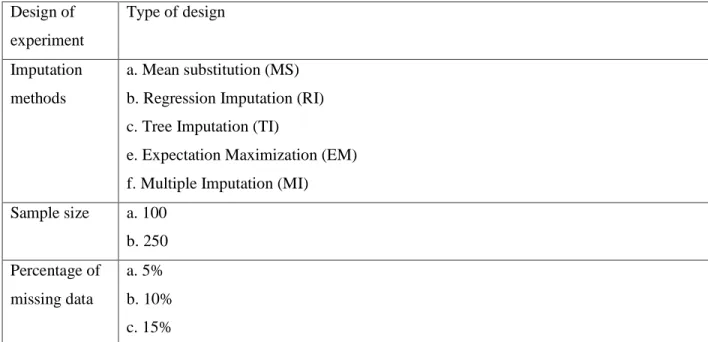
5.3 The Design of the Experiments ...99
5.3.1 Experiment 1: First-order Model ... 99
5.3.2 Experiment 2: Second-order Model ... 99
5.4 The Experimental Procedures ...101
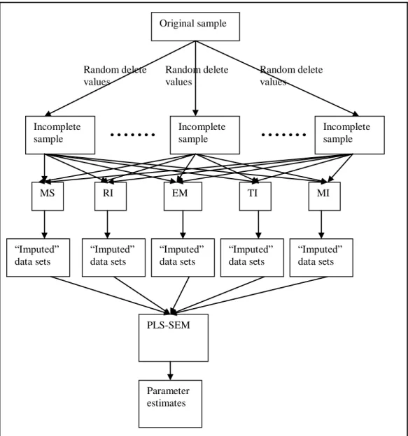
5.4.1 Step 1: Generating the missing data sets ... 102
5.4.2 Step 2: Applying the imputation methods to generate “imputed” data ... 106
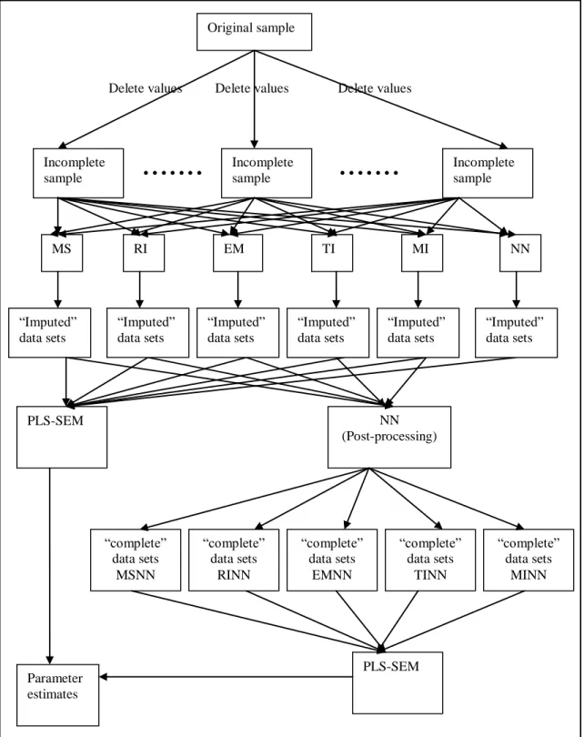
5.4.3 Step 3: Applying a Neural Network as a post-processor for the “imputed” data sets obtained from the statistical methods of data imputation in Step 2 for experiments involving MNAR ... 110
5.4.4 Step 4: Fitting the PLS-SEM with “imputed” and “complete” data sets and comparing the results ... 111
5.5 Criteria for Evaluation...112
5.6 Chapter Summary...114
CHAPTER 6: RESULTS 6.1 Introduction ...115
6.2 Results of Experiment 1: First-Order Model ...116
6.2.1 Comparison of Imputation Methods for MCAR Data ... 117
6.2.1.1 Factor Loadings ... 118
6.2.1.2 Regression Coefficients ... 120
6.2.1.3 The Coefficient of Multiple Determinations (R2) ... 125
6.2.1.4 Standard Error ... 126
6.2.1.5 Correlation Coefficient ... 129
6.2.2 Comparison of Imputation Methods for MNAR Data ... 132
6.2.2.1 Factor Loadings ... 133
vii
6.2.2.3 The Coefficient of Multiple Determinations (R2) ... 140
6.2.2.4 Standard Error ... 143
6.2.2.5 Correlation Coefficient ... 145
6.3 Results of Experiment 2: Second-Order Model ...148
6.3.1 Comparison of Imputation Methods for MCAR data ... 148
6.3.1.1 Factor Loadings ... 149
6.3.1.2 Regression Coefficients ... 151
6.3.1.3 Coefficient of Multiple Determinations (R2) ... 154
6.3.1.4 Standard Error ... 156
6.3.1.5 Correlation Coefficient ... 158
6.3.2 Comparison of Imputation Methods for MNAR ... 160
6.3.2.1 Factor Loadings ... 162
6.3.2.2 Regression Coefficients ... 164
6.3.2.3 The Coefficient of Multiple Determinations (R2) ... 166
6.3.2.4 Standard Error ... 168 6.3.2.5 Correlation Coefficients ... 170 6.4 Chapter Summary...172 CHAPTER 7: DISCUSSION 7.1 Introduction ...173 7.2 Rankings ...175
7.2.1 Mean Substitution and Mean Substitution followed by a Neural Network update 180 7.2.2 Regression Imputation and Regression Imputation followed by a Neural Network update ... 182
7.2.3 Expectation Maximization and Expectation Maximization followed by a Neural Network update ... 184
7.2.4 Tree Imputation and Tree Imputation followed by a Neural Network update 185 7.2.5 Multiple Imputation and Multiple Imputation followed by a Neural Network update 186 7.2.6 Neural Network Imputation ... 187
viii
7.3 Pattern of findings ...189
7.3.1 Evaluating the effects of the proportion of missing values ... 190
7.3.2 Evaluating effects of sample sizes ... 192
7.3.3 Evaluating effects of post-processing procedure using Neural Network .... 194
7.4 Chapter Summary...197
CHAPTER 8: CONCLUSIONS AND FUTURE WORK 8.1 Summary of Research ...198
8.2 Limitations and Suggestions for Future Work ...200
REFERENCES ...205
APPENDIX A ...221
APPENDIX B ...236
ix
LIST OF FIGURES
Figure 2.1: Six prototypical missing data patterns. ... 16
Figure 3.1: Example of a PLS-SEM model. ... 51
Figure 4.1: A three-input, one-output NN with two neurons in the hidden layer. 63 Figure 4.2: Single input neuron. ... 65
Figure 4.3: Multiple input neuron. ... 66
Figure 4.4: Architecture of single layer perceptron. ... 70
Figure 4.5: MLP architecture. ... 71
Figure 4.6: Back-propagation neural network. ... 73
Figure 5.1: ECSI model. ... 90
Figure 5.2: ECSI and PLS estimates (loadings, regression coefficients and R2 values) ... 94
Figure 5.3: The second-order model. ... 100
Figure 5.4: Experimental procedure for Missing Completely at Random. ... 107
Figure 5.5: Experimental procedure for Missing Not at Random. ... 109
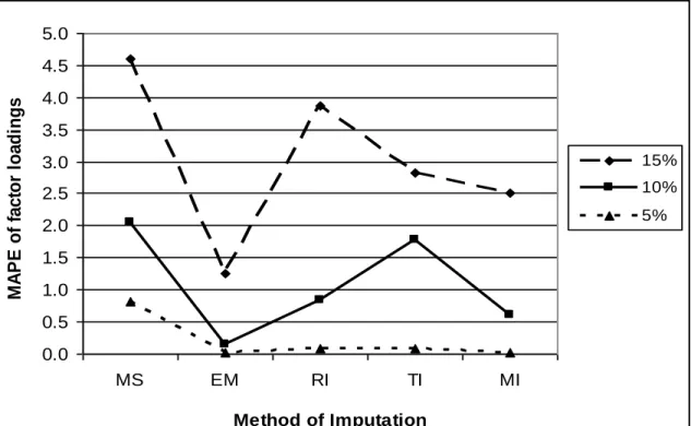
Figure 6.1: Mean absolute percentage error for factor loadings for PERQ3 (n=100). ... 118
Figure 6.2: Mean absolute percentage error for factor loadings for PERQ3 (n=250). ... 119
Figure 6.3: Mean absolute percentage error for regression coefficients for IMAG --> CUEX (n=100). ... 121
Figure 6.4: Mean absolute percentage error for regression coefficients for IMAG --> CUEX (n=250). ... 122
Figure 6.5: Mean absolute percentage error for regression coefficients for CUSA --> CUCO (n=100). ... 124
x
Figure 6.6: Mean absolute percentage error for regression coefficients for CUSA
--> CUCO (n=250). ... 124
Figure 6.7: Mean absolute percentage error for R2 for PERV (n=100)... 125
Figure 6.8: Mean absolute percentage error for R2 for PERV (n=250). ... 126
Figure 6.9: The standard error for CUSA1 (n=100) ... 127
Figure 6.10: The standard error of CUSA1 at n=250 ... 128
Figure 6.11: The correlation coefficients for CUSA1 (n=100). ... 130
Figure 6.12: The correlation coefficients for CUSA1 (n=250) ... 131
Figure 6.13: Mean absolute percentage error (MAPE) for the factor loadings for IMAG2 (mnar12 data). ... 137
Figure 6. 14: Mean absolute percentage error (MAPE) for the factor loadings for IMAG2 (mnar910 data). ... 137
Figure 6.15: Mean absolute percentage error (MAPE) for the regression coefficient of IMAG --> CUSL (mnar12 data). ... 139
Figure 6.16: Mean absolute percentage error (MAPE) for the regression coefficient for IMAG --> CUSL (mnar910 data). ... 139
Figure 6.17: Mean absolute percentage error (MAPE) for factor loading of CUSL3 on CUSL (n=100). ... 150
Figure 6.18: Mean absolute percentage error (MAPE) for factor loading for CUSL3 on CUSL (n=250) ... 150
Figure 6.19: The standard error for CUSL1 (n=100) ... 157
Figure 6.20: The standard error for CUSL1 (n=250) ... 157
Figure 6.21: The correlation coefficients for CUSL1 (n=100). ... 159
Figure 6.22: The correlation coefficient for CUSL1 (n=250). ... 160
Figure 7.1: Rankings of methods for first-order model with missing completely at random data (n=100). ... 176
Figure 7.2: Rankings of methods for first-order model with missing completely at random data (n=250). ... 176
Figure 7.3: Rankings of methods for second-order model with missing completely at random data (n=100). ... 177
xi
Figure 7.4: Rankings of methods for second-order model with missing
completely at random data (n=250). ... 177 Figure 7.5: Rankings of methods for first-order model with MNAR data ... 178 Figure 7.6: Rankings of methods for second-order model with MNAR data ... 179
xii
LIST OF TABLES
Table 2.1: Table with missing values ... 12
Table 2.2: Table with missing entries ... 19
Table 3.1: Comparison of PLS-SEM and CB-SEM ... 34
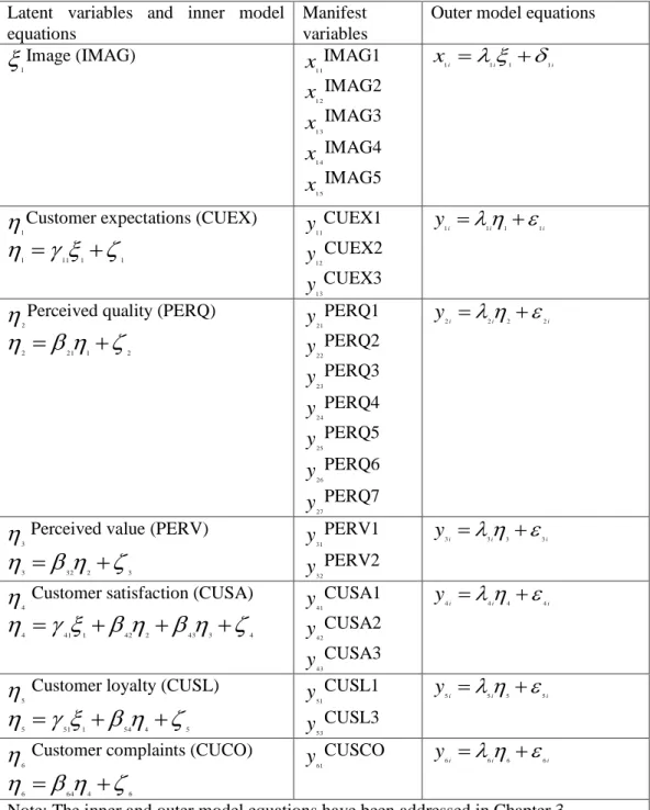
Table 5.1: The latent variables and their manifest variables in the ECSI... 92
Table 5.2: Model variables, parameters and relations ... 95
Table 5.3: Experimental design of study for MCAR ... 103
Table 5.4: Experimental design of study for MNAR ... 105
Table 6.1: The regression coefficients for the first-order ECSI model ... 120
Table 6.2: The MAPE for gamma coefficients for the ECSI model (n=100, percentage of data missing=15%) ... 121
Table 6.3: The MAPE for beta coefficients resulting from data sets with missing data have been imputed by MS (n=100, levels of data missing=5%, 10%, 15%) ... 123
Table 6.4: The correlation coefficients for CUSA1 between imputed values and actual values in MCAR experiment ... 130
Table 6.5: The mean absolute percentage error for factor loadings for the first-order model (mnar12 data) ... 134
Table 6.6: The mean absolute percentage error for factor loadings for the first-order model (mnar910 data) ... 135
Table 6.7: The mean absolute percentage error for R2 for the latent variables (mnar12 data) ... 141
Table 6.8: The mean absolute percentage error for R2 for the latent variables (mnar910 data) ... 141
Table 6.9: The standard error of each MNAR variable for mnar12 data ... 144
xiii
Table 6.11: The correlation of each MNAR variable between the actual and imputed values (mnar12 data) ... 146 Table 6.12: The correlation of each MNAR variable between the actual and imputed values (mnar910 data) ... 146 Table 6.13: The mean absolute percentage error for regression coefficients for second-order model (n=100) ... 153 Table 6.14: The mean absolute percentage error for regression coefficients for second-order model (n=250) ... 153 Table 6.15: The mean absolute percentage error for R2 for latent variables in the second-order model (n=100) ... 154 Table 6.16: The mean absolute percentage error for R2 for latent variables in the second-order model (n=250) ... 155 Table 6.17: The mean absolute percentage error for factor loadings for MNAR variable for second-order model (mnar12 data) ... 163 Table 6.18: The mean absolute percentage error for factor loadings for MNAR variable for second-order model (mnar910 data) ... 163 Table 6.19: The mean absolute percentage error for regression coefficients for the second-order model (mnar12 data) ... 165 Table 6.20: The mean absolute percentage error for regression coefficients for the second-order model (mnar910 data) ... 165 Table 6.21: The mean absolute percentage error for R2 for second-order model (mnar12 data) ... 167 Table 6.22: The mean absolute percentage error for R2 for second-order model (mnar910 data) ... 167 Table 6.23: The standard error for each MNAR variable in the second-order model (mnar12 data) ... 169 Table 6.24: The standard error for each MNAR variable in the second-order model (mnar910 data) ... 169 Table 6.25: The correlation coefficients for each MNAR variable in the second-order model (mnar12 data) ... 170
xiv
Table 6.26: The correlation coefficients for each MNAR variable in the second-order model (mnar910 data) ... 170
1
CHAPTER 1
INTRODUCTION
1.1 Research Background
Standard data analysts are trained to deal with complete data sets that are clean
and reliable in the sense that there are no missing values. In reality, many
researchers commonly face the problem of missing data. For example, in a
clinical trial, the subject may be withdrawn from the study or be unavailable for
the next measurements to be taken. Archaeologists can rarely find complete
data on their subject. In laboratory experiments, certain measurements may not
be made when their magnitudes are below a certain value. In sample survey
practice, the subject may refuse to answer, or forget to respond to, certain
questions. These unwanted incidents produce incomplete data sets that contain
both observed and missing data.
Handling incomplete data is an important issue, especially in modelling, since
this may impact on interpretations of the data or on the models created from the
2
serious problems for researchers because it may result in misleading
conclusions being drawn from a research study (Huanga et al., 2006). A number
of methods have therefore been developed for dealing with such situations
(Roth, 1994). One simple approach to handling missing values is to omit any
incomplete cases from the data set. This approach known as complete case
analysis, may disregard valuable information, especially in a small sample. An
alternative approach to missing values is to use the information available in the
data set to compute the missing values. These approaches are known as
imputation methods.
With a large variety of such methods currently in existence, researchers should
be aware of their best available options for handling missing data in their
studies. There is a recognised need for further investigation into deciding which
method is suitable for a given application. The present research is therefore
designed to compare statistical methods and computational intelligence methods
of data imputation, in terms of their efficacy for partial least squares structural
equation modelling (PLS-SEM) with incomplete data.
Structural equation modelling (SEM) has become a quasi-standard in
management research for analysing the cause-effect relations between latent
constructs (Bollen, 2011). This approach provides a useful and flexible tool for
statistical model building and analysis. There are two types of SEMs: the
covariance-based (CB-SEM), and variance-based partial least squares
3
previous management research has been dominated by the CB-SEM
(Baumgartner & Pieters, 2003) approach. Recently, however, the component
PLS-SEM approach has gained some prominence in management research with the recognition that PLS-SEM’s distinctive methodological features make it a
possible alternative (Hair et al., 2011; Henseler et al., 2009). This is particularly
so for exploratory modelling using SEM (Gefen et al., 2011). In addition, PLS
SEM is robust for relatively small samples (Chin & Newsted, 1999), a particularly
attractive feature for management studies, and can naturally accommodate
formative latent variables (Diamontopoulous & Siguaw, 2006). It therefore,
supports and facilitates investigation of both small and simple to large and
complex path models.
A variety of enhancements to PLS-SEM have been developed in recent years,
including: confirmatory tetrad analysis to empirically test construct measurement
models (Gudergan et al., 2008); guidelines for analysing moderating effects
(Henseler & Fassot, 2010); non-linear effects (Rigdon et al., 2010); and, finite
mixture partial least squares facility to fit and analyse separate models emerging
from the segmentation of the observations (Hahn et al., 2002). PLS SEM is also
relatively attractive as it does not require any distributional properties to be
exhibited by the data but this facility is also now becoming available in CB SEM
packages using the asymptotic distribution free (ADF) facility. These enhancements expand PLS-SEM’s general usefulness as a research tool in
4
PLS also can estimate causal models in many model and data situations (Hair et
al., 2011), especially when complex models and secondary data are involved.
Secondary data, whose use is becoming more and more common in business
research, is typically collected without the benefit of a theoretical framework and
is often not a good match for CB-SEM analysis. In light of the need in CB-SEM
for high-quality and specially developed manifest variables, PLS-SEM may often
be the better choice for structural modelling of secondary data (Rigdon et al.,
2010). Furthermore, PLS is primarily intended for causal-predictive analysis in
situations of high complexity but low theoretical information. Clearly, there are
many areas in business and management where theory is underdeveloped,
which may suit the use of PLS-SEM.
These original features and enhancements that expand PLS-SEM’s general
usefulness make this approach especially useful as a research tool in support of
management studies, and social sciences in general. In this research, the PLS
approach was particularly chosen due to this ability to fit relatively small data
sets, its relative ease of use, extensive functionality and , not least, as it is an
under-researched approach to SEM that is gaining such a large user base
amongst the management studies community.
However, structural equation modelling (CB-SEM and PLS-SEM), was not
designed for dealing with missing data. Complete data is required and
adjustments must be made to the data set when data is incomplete, either by
5
for handling missing data, which combines standard statistical methods of data
imputation with a neural network. Our procedure showed to increase the
accuracy of the estimated values.
1.2 Problem Statement
Most existing literature regarding incomplete data in SEM has dealt only with the
co-variance-based SEM (CB-SEM) (Muthen et al., 1987; Brown, 1994; Arbuckle,
1996; Olinsky et al., 2003; Enders, 2006). Little research has been published in
relation to component-based SEM, also known as PLS-SEM. Only the recent
studies by Cordeiro et al. (2010) and Kristensen and Eskildsen (2010) report the
efficacies of different methods for handling missing data for PLS-SEM. In the
present investigation we therefore focus on PLS-SEM since this approach offers
vast potential for SEM researchers, especially in the marketing and
management information systems disciplines (Henseler et al., 2009).
Statistical methods of data imputation are well researched and are provided as
options by most of the popular statistical software packages. Unlike statistical
methods, computational intelligence methods of data imputation are less widely
used for handling missing data as they require knowledge of coding and
specialized computer software. Nevertheless, it is important to select the best
imputation method to handle missing data since the consequences for not doing
so are reflected in the quality of both, the estimators and the models, fitted to the
6
traditional and other modern statistical methods for handling missing data in
SEM (Brown, 1994; Olinsky et al., 2003), no attempt has so far been reported of
evaluating the performance of estimating missing data using the computational
intelligence methods of data imputation, such as a neural network (NN) in SEM.
The present research compares the imputation methods of mean substitution,
regression imputation, tree imputation, expectation maximization, multiple
imputation and neural network in terms of their efficacy for estimating missing
data with PLS-SEM.
On the other hand, there has been little discussion of the strategies that can be
used to combine a number of known methods for handling missing data. This
thesis aims to propose a novel procedure that combines NN and other statistical
methods of data imputation for handling missing data. Through PLS-SEM, the
performance of various imputation methods applied in this study is compared in
terms of their ability to produce values for fitted structural equation models in
the vicinity of the correct values under different types of missing data - missing
completely at random (MCAR) and missing not at random (MNAR).
According to Brown (1994), there could be more critical problems inherent in the
situation in which the data is MNAR rather than MCAR. There is therefore a
need to investigate the impact of MNAR on the fitted PLS-SEM model,
specifically to identify which method of data imputation is suitable for handling
7 1.3 Research Objectives
The purpose of this research is to compare some of the standard methods of
data imputation in handling incomplete MCAR and MNAR data. A comparison is
made of the accuracy of the methods in modelling data from a customer
satisfaction market survey study using PLS-SEM. The specific objectives of this
research are:
a) to describe and compare the performance of five missing data methods,
namely: mean substitution, regression imputation, expectation
maximization, tree imputation and multiple imputation, in handling
incomplete MCAR data for PLS-SEM;
b) to describe and compare the performance of six missing data methods,
namely, mean substitution, regression imputation, expectation
maximization, tree imputation, multiple imputation and neural network, in
handling incomplete MNAR data;
c) to investigate the effect of two different sample sizes, in particular 100
cases and 250 cases, to illustrate the situation of both small and large
samples in handling incomplete MCAR data;
d) to investigate the effect of the varying rates of missing observations,
particularly the effect of 5%, 10% and 15% missing data rates for MCAR
on the precision of the PLS-SEM estimates;
e) to propose a novel procedure resulting from combining a neural network
with the other five standard statistical methods of data imputation, to deal
8
To accomplish this, the published customer satisfaction model (Tenenhaus et
al., 2005) and data, are used as the baseline for each of the experiments.
1.4 Significance of Findings
Although a great deal of research has been conducted in comparing the best
ways of approximating missing values, no method for handling missing data can,
up to the present, be deemed better than others in all situations. This thesis will
contribute to building this knowledge by identifying suitable methods for handling
missing data with particular missing data mechanisms in SEM applications.
In Chapter 2, we offer a simple clarification of various methods for handling
missing data by classifying them in two categories: case deletion and imputation
method. We aim to assist researchers from a variety of disciplines, including
management, psychology, sociology, education, medicine and marketing, to
plan more informative studies by considering the possible effects of missing data
on their ability to reach valid and replicable inferences with modelling using
PLS-SEM.
Since most statistical packages require the use of complete data before
conducting any procedure for data analysis, the use of missing data methods
can ensure a consistency of results across analysis which cannot be fully
9
one or two approaches for dealing with missing data. This is the case with
PLS-SEM software which typically offers listwise or pairwise deletion and mean
substitution. These have been shown to yield biased estimates, especially when
the missing data is MNAR (Olinsky et al., 2003; Ismail, 2003). Even deleting
incomplete cases from the data set, when applying listwise and pairwise, may
lead to a loss of significant information for the fitting process, especially in small
samples. In this thesis, we therefore seek to provide a step-by-step process
involved in using methods of data imputation, together with the rationale of the
proposed process.
More importantly, this study will focus on applying partial least squares with
structural equation modelling, in order to assist researchers who face the
problem of missing data in small sample sizes when they do not have a priori
distributional assumptions. A small sample will limit the performance of
imputation methods based on modelling the distribution of missing data.
Compared to the existing methods, the use of a new method of data imputation
with less bias and more consistent results may contribute to the success of
10 1.5 Thesis Outline
The remainder of this thesis is structured as follows:
Chapter 2 presents the missing data patterns and mechanisms as described by
Rubin (1976) and Little and Rubin (2002). These are the seminal papers that
established a universal classification system for missing data which is widely
used in the research literature today. A review of the main methods of data
imputation encountered in published research articles or in standard statistical
software packages is also provided.
Chapter 3 compares the two approaches in SEM: PLS-SEM and CB-SEM. A
review of studies that apply PLS-SEM in various areas has also been given. This
chapter also discusses previous studies which offer examples of handling
missing SEM data. Finally, the last section of this chapter provides an outline of
the PLS-SEM algorithm.
Chapter 4 presents the basic foundation of neural networks, learning rules and
its architecture. The chapter also investigates the use of neural network for
prediction, specifically in estimating the missing values.
In Chapter 5, the data set used in this thesis is presented, together with the
design of the experiments, the experimental procedure and the criteria for
11
data, a combination of standard statistical imputation method with neural
network, thereafter are refer this procedure as the post-processing procedure.
Chapter 6 discusses the experimental results. In the first section, we report on
the experiments conducted using MCAR and MNAR data that are fitted to the
first-order customer satisfaction (ECSI) model. The subsequent section presents
the experiment carried out with MCAR and MNAR data fitted to the second-order
model revised from this customer satisfaction model.
Chapter 7 discusses the major findings of this research. In this chapter, the
results and related graphs are discussed. The first section presents the
performance rankings of the five imputation methods when estimating the
first-order PLS-SEM model and the second-first-order PLS-SEM model with missing data
under the MCAR mechanism and those of the eleven imputation methods when
estimating the same models under the MNAR mechanism. The subsequent
sections present the efficacy of each method in comparison to the other
imputation methods, both as a stand-alone procedure and a composite
post-processing procedure. Finally, the findings are summarized in the last section.
Chapter 8 concludes the thesis with a summary of the study and offers insights
into the possibilities for further research that could be conducted in this area of
12
CHAPTER 2
MISSING DATA
2.1 Introduction
Missing data in a database may arise due to various reasons, including data
entry errors or non-response to items during the process of data collection.
Table 2.1 illustrates a database consisting of four variables - age, gender,
income and educational level - where the values for some variables are missing.
For instance, the income and age for the second and third records respectively
are unavailable.
Table 2.1: Table with missing values
Age Gender Income Educational level
25 Male 2000 B.Sc.
33 Female M.Sc.
Female 4500 Ph.D.
13
Thus the question arises, how do we know the income for the second record?
Similarly, how do we know the age for the third entry? Are there any
mechanisms to predict or approximate the missing data in the database?
A number of methods have been developed for dealing with these questions,
and extensive research has been carried out to discover different ways of
approximating the missing values. Prior to the 1970s, the issue of missing data
was addressed by editing (Schafer & Graham, 2002), whereby a missing item
could be logically inferred from other data that had been observed. Dempster,
Laird and Rubin (1977) formulated the Expectation Maximization (EM) algorithm
that led to the full use of Maximum Likelihood (ML) methods in resolving the
missing data problem. Little and Rubin (2002) later introduced the Multiple
Imputation (MI) approach. Multiple Imputation would not have been possible
without the advancements in computing power (Schafer & Olsen, 1998) as they
are computationally intensive.
Since about 2000, computational intelligence methods of data imputation using
machine learning approaches have been developed, but these methods are not
widely used as they require knowledge of computer coding and computer
software. It can be suggested that, because of the longstanding use of traditional
statistical methods of data imputation, it has taken some time for these
computational methods to gain general favour even though they are as
14
Missing data is a very common problem in empirical research (Downey & King,
1998) especially when conducting surveys, because these usually involve
multiple responses from a large number of respondents (Quinten & Raaijmakers,
1999). However, this topic has received less coverage in business and
management, even though it is common for many researchers in this area to
utilize surveys as their primary or secondary research methodology. On the
other hand, certain fields such as organizational behaviour (Roth et al., 1999),
statistics (Stinebrickner, 1999), psychometrics (Brown, 1983; Newman, 2003)
and social science (Fricker & Tourangeau, 2010) have paid more attention to the
issue. As a consequence, approaches to data analysis that are regularly used by
business and management scholars have not employed these newer methods of
data imputation. One of the purposes of the present research, therefore, is to
familiarize empirical business and management researchers with the key issues
of dealing with missing data.
In this chapter we present the mechanisms and patterns of missing data as
described by Rubin (1976) and Little and Rubin (2002). Rubin established a
universal classification scheme for missing data problems that is widely used in
the literature today. Furthermore, we describe the main methods of data
imputation that have been used in published management research articles or
15 2.2 Missing Data Patterns
As a starting point, it is useful to distinguish between missing data patterns and
missing data mechanisms. These terms have very different meanings but
researchers sometimes use them interchangeably. A missing data pattern refers
to the configuration of observed and missing values in a data set, whereas
missing data mechanisms describe possible relationships between measured
variables and the probability of missing data (Enders, 2010). In other words, a missing data pattern simply describes the location of the “blanks” in the data and
does not explain why the data is missing.
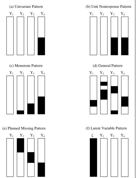
Figure 2.1 below depicts six prototypical missing data patterns proposed by
Enders (2010), with the shaded areas representing the location of missing
values in the data set. The univariate pattern (a) has missing values restricted to
a single variable. This pattern is relatively rare in some disciplines but can arise
in experimental studies. For example, suppose that Y1 through to Y3 are
manipulated variables and Y4 is the incomplete outcome variable. A unit
nonresponse pattern (b) often occurs in survey research, where Y1 and Y2 are
characteristics that are available for every member of the sampling frame, and
Y3 and Y4 are surveys that some respondents refuse to answer. A Monotone
missing data pattern (c) is typically associated with a longitudinal study where
participants drop out and never return. A general missing data pattern (d) is
perhaps the most common configuration of missing data. As seen in Figure 2.1,
16
random pattern. This seemingly random pattern is deceptive because the values
can still be systematically missing.
(a) Univariate Pattern Y1 Y2 Y3 Y4
(b) Unit Nonresponse Pattern Y1 Y2 Y3 Y4
Y1 Y2 Y3 Y4 Y1 Y2 Y3 Y4
(e) Planned Missing Pattern (f) Latent Variable Pattern
Y1 Y2 Y3 Y4 ξ Y2 Y3 Y4
(d) General Pattern (c) Monotone Pattern
17
A planned missing data pattern (e) corresponds to the basic idea of three-form
questionnaire design (Graham et al., 1996). The basic idea this design is to
distribute questionnaires across different forms and to administer a subset of the
forms to each respondent. For example, the design leads to the distribution of
four questionnaires across three forms, such that each form includes Y1 but is
missing Y2, Y3, or Y4. Planned missing data patterns are useful for collecting a
large number of questionnaire items while at the same time reducing respondent
burden. Finally, the Latent Variable pattern (f) is designed for latent variable
analyses where the values of the latent variables are missing for the entire
sample. For example, a confirmatory factor analysis model uses a latent factor
to explain the associations among a set of manifest variables (e.g., Y1 through
Y3), but the factor scores themselves, ξ, are completely missing.
From a practical point, distinguishing missing data patterns is no longer so
important because multiple imputation methods are well suited for any missing
data pattern (Enders, 2010). The present research focuses primarily on general
missing data pattern (d) because this pattern works well with almost all methods
of data imputation and is commonly used in survey research.
18 2.3 Missing Data Mechanisms
Little and Rubin (2002) distinguish between three missing data mechanisms:
Missing Completely at Random (MCAR), Missing at Random (MAR) and Missing
Not at Random (MNAR), as described below.
2.3.1 Missing Completely at Random (MCAR)
Data is said to be MCAR when the probability that an observation is missing
does not depend on either observed or unobserved values. In other words, the
probability that an observation is missing is not associated with any variables
that have been measured or with any variables that are not measured. For this
reason MCAR data is equivalent to a simple random sample of the full data set.
The missing data for a variable age, for example, is said to be MCAR if the
missing value is unrelated to the variable age itself or to the values of any other
variable in the database, whether missing or observed (Allison, 2002).
In this situation, cases with complete data are indistinguishable from cases with
incomplete data. In Table 2.2 the missing value in x3 is said to be MCAR if the
value missing does not depend on the values in x1,x2, x4 and x5 and also on x3
19 Table 2.2: Table with missing entries
Observation x1 x2 x3 x4 x5 1 25 3.5 5000 -3.5 2 6.9 5.6 0.5 3 45 3.6 9.5 1500 46.5 4 27 9.7 7.1 3000
2.3.2 Missing at Random (MAR)
Missing at Random requires that the cause of missing data be unrelated to the
missing values themselves. Although, the cause may be related to other
observed variables (Schafer, 1997). MAR occurs when cases with missing data
are different from the observed cases but the pattern of missing data is
predictable from other observed variables. For example, if the probability of
missing data on income depends on marital status but, within each category of
marital status, the probability of missing income is unrelated to the value of
income, income in this case is considered as MAR (Little & Rubin, 2002).
In this case, the cause of the missing data is due to external influence and not to
the variable itself (Schafer & Graham, 2002). In Table 2.2, the missing value in
x3 is said to be MAR if the value missing depends on the values in x1,x2, x4 and
20 2.3.3 Missing Not at Random (MNAR)
Missing Not at Random (MNAR) implies that the missing data mechanism is
related to the missing values. For example, if high income households are less
likely to report their income even after adjusting for other variables, then the
probability of missing income is said to be MNAR (Little & Rubin, 2002). In this
case, the pattern of missing data is not predictable from other variables in the
data set. MNAR data is the most difficult to approximate and model compared to
the two other missing data mechanisms (Rubin, 1987), therefore thorough
strategies for dealing with MNAR data are needed. In Table 2.2, the missing
value in x3 is said to be MNAR if the missing value in x3 depends on the values
in variable x3 itself.
2.4 Strategies for Dealing with Missing Data
There are currently various methods for dealing with missing data available in
statistical packages (Yansaneh et al., 1998). These range from simple methods
such as data deletion to methods employing sophisticated statistical or
computational strategies. The following discussion reviews some of the most
commonly provided methods of data imputation, starting with the simple
21 2.4.1 Listwise Deletion
This is the default procedure in the SAS, SPSS and MINITAB statistical
packages. Only those cases with no missing values are used, so it is the easiest
method for handling missing data (Roth, 1994). The disadvantage with this
procedure is the discarding of the information contained in incomplete cases.
When there are only a few cases with missing values, little information contained
in the incomplete cases is lost, but much is lost when there are many cases with
missing values. In such circumstances, treating missing data using this method
is plausible only if such data is a small proportion of the available complete data
in the database (Little & Rubin, 2002). Otherwise, using this method when the
missing data represents a relatively high proportion may lead to biased results
and findings.
2.4.2 Pairwise Deletion
Also known as available case analysis, pairwise deletion is a simple alternative
that can be used for many linear models, including linear regression, factor
analysis and more complex structural equation models. It is well known, for
example, that a linear regression can be estimated using only the sample means
and covariance matrix or, equivalently, the means, standard deviations, and
correlation matrix. The idea of pairwise deletion is to compute each of these
summary statistics using all the cases that are available. For example, to
22
data present for both X and Z are used. Once the summary measures have
been computed, they can be used to calculate the parameters of interest, for
example, regression coefficients. Although this may seem a sound idea in
principle, it has many potential inconsistencies, and its use is rarely justified in
practice. For example, different means may be used to generate each
correlation of variable X and Y in a matrix. Currently, different statistical
packages may calculate pairwise covariances using different formulas and so
may yield different results for what is ostensibly the same correlation. Without
stronger justification, this approach is probably best avoided. Taking Table 2.2
as an example of pairwise deletion method, observation number 1 will be used
whenever there is any analysis that does not involve variable x3.
2.4.3 Imputation Methods
The previous two (listwise and pairwise) methods of handling missing data make
use of the data that are available only. However, in some instances it might be
prudent to fill-in (impute) the missing cases. By imputing the missing values, the
researcher is then able to use SEM or any standard statistical techniques that
require complete data sets. Imputation methods involve replacing missing values
with estimated values based on information available in the data set. Imputation
methods can be either single or multiple. In single imputation the missing value
is replaced with one imputed value, while in multiple imputation several values
are used. The following section describes how each of the imputation methods
23 2.4.3.1 Mean Substitution (MS)
The most popular method of imputation is the substitution of a missing entry by
the corresponding variable's mean value. This is referred to as Mean
Substitution (MS). The popularity of MS is probably the result of its simplicity.
However, an important limitation of MS is that the variance of the resulting
imputed data systematically underestimates the real variance (Little & Rubin,
2002) suggesting. Employing the MS method in Table 2.2, the missing values in
variable x3 will be substituted by averaging the values of the available values in
this variable. In this case the value will be
4
.
7
3
1
.
7
5
.
9
6
.
5
2 1
n
x
i i (2.1)2.4.3.2 Regression Imputation (RI)
In the regression imputation (RI), a regression equation is developed based on
complete case data for a given variable, treating the missing variable as the
dependent variable and using all other relevant variables in the data set as
predictors. For the cases where the value is missing, its value is predicted or
approximated based on the regression equation developed in terms of these
other variables (Little & Rubin, 2002). It is noted that with this method, a
24
other variables are used as independent variables. The process is repeated
sequentially for variables with missing values, which means that for a variable xj
with missing values, a model is fitted using cases with observed values for the
other variables.
Using the regression method in Table 2.2 to approximate the missing value in
observation 1, a regression equation will be fitted in terms of variables x1, x2, x4,
and x5. The equation can be formulated as
x
b
x
b
x
b
x
b
b
x
3
0
1 1
2 2
4 4
5 5 (2.2)The fitted model includes the regression parameter estimates bi, the regression
coefficients. Equation 2.2 can then be used to estimate the missing value by
substituting the corresponding values of x1, x2, x4, and x5 into the equation.
When regression imputation is used to fill-in missing values on the dependent
variables, those with missing values on the dependent variables will be perfectly
predicted. Thus, inflating the predictive power of the model (Enders, 2010). On
the other hand, if regression imputation is used to fill-in missing values on the
independent variables, the imputed values will be perfectly correlated with the
other variables in the model. Thus, increasing multicolinearity among the
25 2.4.3.3 Tree-based Imputation (TI)
There are two basic types of tree-based missing data method that can be
characterized in terms of the scale of measurement of the response variable
(Breiman et al., 1984; Quinlan, 1989; Mesa et al., 2000), namely, classification
tree and regression tree. In the former, the variable with missing data is
assumed to be a nominal variable, whereasunder the regression tree model it is
numerical.
Handling missing values using the classification tree imputation method is very
straightforward. First, a variable with missing data is taken, together with the
independent variables without missing entries. A classification/regression tree is
then built which represents the distribution of the response variable in terms of
the values of independent variables. The missing values in the response
variable are then imputed using an appropriate approach, for instance, mean substitution, based on the “complete data" entities in the same node (Mesa et
al., 2000).
A second option is to impute the data using the regression tree where the
procedure is just same like regression imputation. A simple example would be to
employ conventional regression in which a predictor with the missing data is
regressed on other predictors with which it is likely to be related. The resulting
regression equation can then be used to impute what the missing values might
26 2.4.3.4 Neural Networks Imputation (NN)
There is little guidance in the literature about the use of neural networks (NN) in
handling missing data problems. It is a relatively new computational method that
is based on conceptual models of the anatomy of the brain. NN can modify its
behaviour in response to its environment. In other words, it learns from
experience and generalizes from previous examples when applying to new
situations. In the context of missing data, NN can be trained on data sets with no
missing data and then used to impute values for those cases where data is
missing (Wilmot & Shivananjappa, 2001).
An advantage of this method is that it does not make any distributional
assumptions about the data set. In addition, several alternative estimates for the
missing values can be generated from the network repetition with a difference
hidden layer (Gupta & Lam, 1996). A disadvantage is that the method is
complex and not easy to understand. Since NN are also computationally
intensive, relatively few researchers use it for their data.
Lam and Gupta (1996) were the first to use NN to reconstruct missing values in
multivariate data, comparing the results obtained with MS and RI. This
demonstrated that NN consistently outperformed the other two methods. The
study by Wilmot and Shivananjappa (2001) compared the use of NN to hot deck
27
accurate imputed values than the hot deck procedure. They also claimed that
NN was more difficult and time-consuming to construct than hot deck.
Experience in the development and use of NN is therefore needed to obtain and improve the performance of NN. In addition, Nordbotten’s study (1998) involving
agricultural data discussed experiments using NN to increase the effectiveness
of statistical editing and imputation. A recent study by Marwala (2009), which
investigated medical data, compared the use of NN and the genetic algorithm
(GA). Their results show that the NN model yields higher accuracy than when
using GA. The low accuracy of the GA may be attributed to the fact that the GA
converges slowly, hence the global optimum may not have been obtained. The
details of the NN imputation method are presented in Chapter 4.
2.4.3.5 The Expectation Maximization Algorithm (EM)
The Expectation Maximization (EM) algorithm is a procedure that is particularly
important for missing data analyses. The origins of EM date back to the 1970s
(Orchard & Woodbury, 1972; Dempster et al., 1977). The early applications
primarily focused on estimating a mean vector and a covariance matrix with
missing data, but methodologists have since extended the algorithm to address
a variety of difficult complete data estimation problems, including multilevel
models (Liang & Bentler, 2004).
The EM algorithm is a two-step iterative procedure that consists of an E-step
28
The estimation process for a mean vector and a covariance matrix with missing
data are described below.
The iterative process starts with an initial estimate of the mean vector and the
covariance matrix, perhaps from listwise deletion. The E-step uses the elements
in the mean vector and the covariance matrix to build a set of regression
equations that predict the incomplete variables from the observed variables. The
purpose of the E-step is to fill in the missing values. The M-step subsequently
applies standard complete data formulas to the filled-in data to generate updated
estimates of the mean vector and the covariance matrix. The algorithm carries
the updated parameter estimates forward to the next E-step, where it builds a
new set of regression equations to predict the missing values. The subsequent
M-step then re-estimates the mean vector and the covariance matrix. EM
repeats these two steps until convergence is obtained. Convergence occurs
when the change of the parameter estimates from iteration to iteration becomes
negligible. The main steps involved in the EM approach are summarized below
(Little & Rubin, 2002):
1. Replace missing values by estimated values.
2. Estimate parameters.
3. Re-estimate the missing values using the estimated parameters.
4. Iterate between step 2 and 3 until convergence.
The advantage of the EM approach is that it has well known statistical properties
29
and MS because it assumes that incomplete cases have data missing at random
rather than missing completely at random (Allison, 2002; Rubin, 1987). The
disadvantage of the EM approach is that it can be very slow to converge with
large proportions of missing data (Allison, 2002; Rubin, 1987).
2.4.3.6 Multiple Imputation (MI)
Multiple Imputation (MI) combines the strength of a maximum likelihood
approach with the EM and creates five to ten data sets in which raw data are
generated that can be used to substitute the missing data (Schafer, 1999). The
data from the imputed data set is then pooled and parameters are estimated. MI
works by generating a maximum likelihood based covariance matrix and vector
of means, similar to the EM algorithm. MI takes the process one step further by
introducing statistical uncertainty into the model and using that uncertainty to
emulate the natural variability among cases encountered in a complete data set.
MI then imputes actual data values to fill in the incomplete data points in the
data matrix (Little & Rubin, 2002).
The data analyst then analyses each data set, collects the results from the
analyses, and summarizes them into one summary set of findings. For instance,
a researcher may wish to perform a multiple regression analysis on a data set
with incomplete data. The researcher would run MI, generate ten imputed data
sets, and run the multiple regression analysis on each of the ten data sets. The
30
into a single summary. MI has several advantages. It is fairly well understood
and robust to violations of non-normality of the variables used in the analysis. It
outputs complete data matrices and is clearly superior to listwise, pairwise and
MS in handling missing data in most cases (Olinsky et al., 2003). The
disadvantages include the time required to impute five to ten data sets, fitting
models for each data set separately, and recombining the model results into one
summary.
MI appears to be one of the most applicable method for general purpose
handling of missing data in multivariate analysis. The basic procedures of MI, as
presented in Little and Rubin (2002), are:
1. Impute missing values using an appropriate model that incorporates
random variation.
2. Repeat this M times (usually 3-5 times), producing M complete data sets.
3. Perform the desired analysis on each data set using standard complete
data methods.
4. Average the values of the parameter estimates across the M samples to
produce a single point estimate.
5. Calculate the standard errors by (a) averaging the squared standard
errors of the M estimates (b) calculating the variance of the M parameter
estimates across samples, and (c) combining the two quantities using a
31
MI is particularly flexible for a wide variety of linear and nonlinear models. It has
been observed that MI outperforms listwise and pairwise in most cases (Schafer,
1997; Allison, 2002).
2.5 Chapter Summary
Missing data refers to the case that some of the components of the data vectors
are not available for all data items in the database, or may not even be
applicable or defined. This creates various problems in analysing and
processing of data in databases. Currently, there are various methods of dealing
with missing data. Each of the methods have their pros and cons. Due to the
availability of software and advancement of computational power, computational
intelligence methods of data imputation such as neural networks have been
32
CHAPTER 3
PARTIAL LEAST SQUARES
STRUCTURAL EQUATION
MODELLING
3.1 Introduction to Structural Equation Modelling and Partial Least Squares
The advent of SEM with latent variables has changed the nature of research in
many areas. Since Jöreskog's (1967) seminal work on maximum likelihood
factor analysis and its later extensions to the estimation of structural equation
systems (Jöreskog, 1972), SEM has become one of the most important methods
for empirical research. It has been applied extensively in psychology
(MacCallum & Austin, 2000), in management (Williams et al., 2003), and in
marketing (Baumgartner & Pieters, 2003). Currently, there are two general
33
as implemented in, for example, LISREL, AMOS and EQS, and the
variance-based structural equation modelling, known as Partial Least Squares
(PLS-SEM).
CB-SEM focuses on estimating a set of model parameters so that the theoretical
covariance matrix implied by the system of structural equations is as close as
possible to the empirical covariance matrix observed within the fitted model.
When fitted using maximum likelihood (ML), this estimation requires a set of
assumptions to be fulfilled, such as a multivariate normal distribution of the
observed indicators and sufficient sample size. If these assumptions are
violated, PLS-SEM (Hair et al., 2005; Wold, 1975) would be a suitable option for
researchers. Unlike CB-SEM, a PLS-SEM analysis does not require any
distributional assumptions to be fulfilled (Wold, 1975) and is able to provide
robust and accurate fits for relatively small sample sizes (Tenenhaus et al.,
2005).
3.1.1 Comparison of PLS-SEM and CB-SEM
According to Gefen et al. (2000), the CB-SEM approach differs from the
PLS-SEM approach in several areas. These approaches differ in the analyses of their
objectives, their underlying statistical assumptions, and the nature of the fit
statistics they produce (Gefen et al., 2000). The CB-SEM is based on the
34
likelihood (ML) function to minimize the difference between the sample
covariance and those predicted by the theoretical model. In contrast, the
PLS-SEM algorithm minimizes the variance of all the dependent variables instead of
explaining the covariance. Table 3.1 below summarizes the characteristics of the
PLS-SEM approach and compares it with CB-SEM, adapted from Chin and
Newsted (1999).
Table 3.1: Comparison of PLS-SEM and CB-SEM
Feature PLS-SEM CB-SEM
Objective Prediction-oriented Parameter-oriented
Approach Variance-based Covariance-based
Assumption Predictor specification
(non-parametric)
Multivariate normal
distribution and independent observations (parametric)
Parameter estimates Consistent as indicators and
sample size increase
Consistent
Latent variable scores Explicitly estimated Indeterminate
Epistemic relationship between an LV and its measures
Can be modelled in either formative or reflective measurement models
Only with reflective models
Implications Optimal for prediction
accuracy
Optimal for parameter accuracy
Model complexity Large complexity Small to moderate
complexity
Sample size Power analysis based on the
portion of the model with the largest number of predictors. Minimal recommendations range from 30 to 300 cases.
Ideally based on power analysis specific model. Minimal recommendations range from 200 to 800.
35
Overall, PLS-SEM can be an adequate alternative to CB-SEM if the problem has
the following characteristics (Chin, 1998; Chin & Dibbern, 2007):
The phenomenon to be investigated is relatively new and measurement models need to be newly developed.
The structural equation model is complex with a large number of latent variables and indicator variables.
Relationships between the indicators and latent variables have to be modelled in different modes (i.e., formative and reflective measurement
models).
The conditions relating to sample size, independence, or normal distribution are not met, and/or
Prediction is more important than parameter estimation.
Notwithstanding how accommodating PLS-SEM can be, CB-SEM is a more
established approach with recognized goodness of fit (GoF) metrics and better
parameter accuracy, and is therefore more frequently accepted for rigorous
model validation purposes (Henseler & Fassott, 2010). Although comparisons of
methods provide some evidence of PLS-SEM' favourable behaviour in light of its
distribution-free character, CB-SEM can use alternative approaches that are
distribution-free, such as Asymptotic Distribution Free (ADF) model fitting. Both
approaches have particular advantages and disadvantages that qualify them for
specific settings. Consequently, researchers should carefully analyse the design