Support Vector Ordinal Regression
Wei Chu [email protected]
Center for Computational Learning Systems, Columbia University, New York, NY 10115 USA
S. Sathiya Keerthi [email protected]
Yahoo! Research, Media Studios North, Burbank, CA 91504 USA
Abstract
In this paper, we propose two new support vector approaches for ordinal regression, which optimize multiple thresholds to define parallel discriminant hyperplanes for the ordinal scales. Both approaches guarantee that the thresholds are properly ordered at the optimal solution. The size of these optimization problems is linear in the number of training samples. The SMO algorithm is adapted for the resulting optimization problems; it is extremely easy to implement and scales efficiently as a quadratic function of the number of examples. The results of numerical experiments on some benchmark and real-world data sets, including applications of ordinal regression to information retrieval and collaborative filtering, verify the usefulness of these approaches.
1
Introduction
We consider the supervised learning problem of predicting variables of ordinal scale, a setting that bridges metric regression and classification, and referred to as ranking learning or ordinal regression. Ordinal regression arises frequently in social science and information retrieval where human preferences play a major role. The training samples are labelled by ranks, which exhibits an ordering among the different categories. In contrast to metric regression problems, these ranks
are of finite types and the metric distances between the ranks are not defined. These ranks are also different from the labels of multiple classes in classification problems due to the existence of the ordering information.
There are several approaches to tackle ordinal regression problems in the domain of machine learning. The naive idea is to transform the ordinal scales into numeric values, and then solve the problem as a standard regression problem. Kramer et al. (2001) investigated the use of a regression tree learner in this way. A problem with this approach is that there might be no prin-cipled way of devising an appropriate mapping function since the true metric distances between the ordinal scales are unknown in most of the tasks. Another idea is to decompose the origi-nal ordiorigi-nal regression problem into a set of binary classification tasks. Frank and Hall (2001) converted an ordinal regression problem into nested binary classification problems that encode the ordering of the original ranks and then organized the results of these binary classifiers in some ad hoc way for prediction. It is also possible to formulate the original problem as a large augmented binary classification problem. Har-Peled et al. (2002) proposed a constraint classifi-cation approach that provides a unified framework for solving ranking and multi-classificlassifi-cation problems. Herbrich et al. (2000) applied the principle of Structural Risk Minimization (Vap-nik, 1995) to ordinal regression leading to a new distribution-independent learning algorithm based on a loss function between pairs of ranks. The main difficulty with these two algorithms (Har-Peled et al., 2002; Herbrich et al., 2000) is that the problem size of these formulations is a quadratic function of the training data size. As for sequential learning, Crammer and Singer (2002) proposed a proceptron-based online algorithm for rank prediction, known as the PRank algorithm.
Shashua and Levin (2003) generalized the support vector formulation for ordinal regression by finding r−1 thresholds that divide the real line intorconsecutive intervals for the r ordered categories. However there is a problem with their approach: the ordinal inequalities on the thresholds, b1 ≤ b2 ≤ . . . ≤ br−1, are not included in their formulation. This omission may result in disordered thresholds at the solution on some unfortunate cases (see section 5.1 for an example). It is important to make any method free of bad situations where it will not work.
one takes only the adjacent ranks into account in determining the thresholds, exactly as Shashua and Levin (2003) proposed, but we introduce explicit constraints in the problem formulation that enforce the inequalities on the thresholds. The second approach is entirely new; it considers the training samples from all the ranks to determine each threshold. Interestingly, we show that, in this second approach, the ordinal inequality constraints on the thresholds are automatically satisfied at the optimal solution though there are no explicit constraints on these thresholds. For both approaches the size of the optimization problems is linear in the number of training samples. We show that the popular SMO algorithm (Platt, 1999; Keerthi et al., 2001) for SVMs can be easily adapted for the two approaches. The resulting algorithms scale efficiently; empirical analysis shows that the cost is roughly a quadratic function of the problem size. Using several benchmark datasets we demonstrate that the generalization capabilities of the two approaches are much better than that of the naive approach of doing standard regression on the ordinal labels.
The paper is organized as follows. In section 2 we present the first approach with explicit inequality constraints on the thresholds, derive the optimality conditions for the dual problem, and adapt the SMO algorithm for the solution. In section 4 we present the second approach with implicit constraints. In section 5 we do an empirically study to show the scaling properties of the two algorithms and their generalization performance. We conclude in section 6.
Notations Throughout this paper we will use x to denote the input vector of the ordinal regression problem and φ(x) to denote the feature vector in a high dimensional reproducing kernel Hilbert space (RKHS) related to x by transformation. All computations will be done using the reproducing kernel function only, which is defined as
K(x, x) = φ(x)·φ(x) (1)
where·denotes inner product in the RKHS. Without loss of generality, we consider an ordinal regression problem withr ordered categories and denote these categories as consecutive integers Y = {1,2, . . . , r} to keep the known ordering information. In the j-th category, where j ∈ Y, the number of training samples is denoted as nj, and thei-th training sample is denoted as xji
b2 b1
y=1 y=2 y=3
b2-1 b2+1 b1-1 b1+1 ξi∗1+1 ξi2 ξi∗2+1 ξi1 f(x) = w φ(x).
Figure 1: An illustration of the definition of slack variables ξ and ξ∗ for the thresholds. The samples from different ranks, represented as circles filled with different patterns, are mapped by w·φ(x)onto the axis of function value. Note that a sample from rankj+ 1 could be counted twice for errors if it is sandwiched bybj+1−1 andbj+ 1 wherebj+1−1< bj+ 1, andthe samples
from rank j + 2, j−1 etc. never give contributions to the threshold bj. wherexji ∈Rd. The total number of training samplesr
j=1nj is denoted asn. bj,j = 1, . . . , r−1 denote the (r−1) thresholds.
2
Approach 1: Explicit Constraints on Thresholds
As a powerful computational tool for supervised learning, support vector machines (SVMs) map the input vectors into feature vectors in a high dimensional RKHS (Vapnik, 1995; Sch¨olkopf and Smola, 2002), where a linear machine is constructed by minimizing a regularized functional. For binary classification (a special case of ordinal regression withr = 2), SVMs find an optimal direction that maps the feature vectors into function values on the real line, and a single opti-mized threshold is used to divide the real line into two regions for the two classes respectively. In the setting of ordinal regression, the support vector formulation could attempt to find an optimal mapping direction w, and r −1 thresholds, which define r −1 parallel discriminant hyperplanes for the r ranks accordingly. For each threshold bj, Shashua and Levin (2003) sug-gested considering the samples from the two adjacent categories, j andj+ 1, for empirical errors (see Figure 1 for an illustration). More exactly, each sample in the j-th category should have a function value that is less than the lower margin bj −1, otherwise w·φ(xji) −(bj −1) is the
error (denoted as ξji); similarly, each sample from the (j+ 1)-th category should have a function value that is greater than the upper margin bj + 1, otherwise (bj + 1)− w·φ(xji+1) is the error (denoted as ξi∗j+1).1 Shashua and Levin (2003) generalized the primal problem of SVMs to ordinal regression as follows:
min w,b,ξ,ξ∗ 1 2w·w+C r−1 j=1 nj i=1 ξij + nj+1 i=1 ξi∗j+1 (2) subject to w·φ(xji) −bj ≤ −1 +ξij, ξij ≥0, for i= 1, . . . , nj; w·φ(xji+1) −bj ≥+1−ξi∗j+1, ξi∗j+1 ≥0, for i= 1, . . . , nj+1; (3)
where j runs over 1, . . . , r−1 and C >0.
A problem with the above formulation is that the natural ordinal inequalities on the thresh-olds, i.e., b1 ≤ b2 ≤ . . . ≤ br−1 cannot be guaranteed to hold at the solution. To tackle this problem, we explicitly include the following constraints in (3):
bj−1 ≤bj, for j = 2, . . . , r−1. (4)
2.1
Primal and Dual Problems
By introducing two auxiliary variables b0 =−∞ andbr = +∞, the modified primal problem in (2)–(4) can be equivalently written as follows:
min w,b,ξ,ξ∗ 1 2w·w+C r j=1 nj i=1 ξij+ξi∗j (5) 1The superscript∗inξ∗j+1
i denotes that the error is associated with a sample in the adjacent upper category
subject to
w·φ(xji) −bj ≤ −1 +ξij, ξij ≥0, ∀i, j; w·φ(xji) −bj−1 ≥+1−ξi∗j, ξi∗j ≥0, ∀i, j;
bj−1 ≤bj,∀j.
(6)
The dual problem can be derived by standard Lagrangian techniques. Let αji ≥ 0, γij ≥ 0,
α∗ij ≥ 0, γi∗j ≥ 0 and µj ≥ 0 be the Lagrangian multipliers for the inequalities in (6). The Lagrangian for the primal problem is:
Le = 12w·w+C r j=1 nj i=1 ξij +ξi∗j −r j=1 nj i=1α j i(−1 +ξij − w·φ(xji)+bj) −r j=1 nj i=1α ∗j i (−1 +ξi∗j +w·φ(x∗ij) −bj−1) −r j=1 nj i=1γijξij − r j=1 nj i=1γ∗ijξi∗j − r j=1µj(bj −bj−1). (7)
The KKT conditions for the primal problem require the following to hold:
∂Le ∂w =w− r j=1 nj i=1 α∗ij −αjiφ(xji) = 0; (8) ∂Le ∂ξji =C−αji −γij = 0, ∀i, ∀j; (9) ∂Le ∂ξi∗j =C−α∗ij −γi∗j = 0, ∀i, ∀j; (10) ∂Le ∂bj =− nj i=1αji −µj + nj+1 i=1 α∗j +1 i +µj+1 = 0,∀j.
Note that the dummy variables associated with b0 and br, i.e. µ1, µr, α∗i1’s andαri’s, are always zero. The conditions (9) and (10) give rise to the constraints 0 ≤ αji ≤ C and 0 ≤ αi∗j ≤ C
respectively. Let us now apply Wolfe duality theory to theprimal problem. By introducing the KKT conditions (8)–(10) into the Lagrangian (7) and applying the kernel trick (1), the dual
problem becomes a maximization problem involving the Lagrangian multipliers α, α∗ and µ:
max α,α∗,µ j,i (αji +α∗ij)− 1 2 j,i j,i (αi∗j−αji)(α∗ij −αj i)K(x j i, xj i) (11)
subject to 0≤αji ≤C, ∀i, ∀j, 0≤α∗ij+1 ≤C, ∀i, ∀j, nj i=1α j i +µj = nj+1 i=1 α ∗j+1 i +µj+1, ∀j, µj ≥0, ∀j, (12)
where j runs over 1, . . . , r −1. Leaving the dummy variables out of account, the size of the optimization problem is 2n−n1−nr (α and α∗) plusr−2 (for µ).
The dual problem (11)–(12) is a convex quadratic programming problem. Once the α, α∗ and µ are obtained by solving this problem, w is obtained from (8). The determination of the
bj’s will be addressed in the next section. The discriminant function value for a new input vector
x is
f(x) =w·φ(x)= j,i
(α∗ij−αji)K(xji, x). (13)
The predictive ordinal decision function is given by arg min
i {i:f(x)< bi}.
2.2
Optimality Conditions for the Dual
To derive proper stopping conditions for algorithms that solve the dual problem and also de-termine the thresholds bj’s, it is important to write down the optimality conditions for the
dual. Though the resulting conditions that are derived below look a bit clumsy because of the notations, the ideas behind them are very much similar to those for the binary SVM classifier case, as the optimization problem is actually composed of r−1 binary classifiers with a shared mapping direction w and the additional constraint (4). The Lagrangian for the dual can be written down as follows:
Ld = 12 j,i j,i(αi∗j−αij)(α∗j i −αj i)K(xji, xj i) +rj=1−1βj(ni=1j αij−ni=1j+1αi∗j+1+µj−µj+1) −j,i(ηijαji +η∗ijαi∗j)−j,i(πij(C−αij) +π∗ij(C−α∗ij))−rj=2−1λjµj − j,i(αji +α∗ij)
where the Lagrangian multipliersηij,ηi∗j,πij,πi∗j and λj are non-negative, whileβ
j can take any value.
The KKT conditions associated withα and α∗ can be given as follows:
∂Ld ∂αji =−f(xji)−1−ηji +πji +βj = 0, πij ≥0, ηji ≥0, πij(C−αji) = 0, ηjiαji = 0, for i= 1, . . . , nj; ∂Ld ∂α∗ij+1 =f(xji+1)−1−ηi∗j+1+π∗ij+1−βj = 0, πi∗j+1 ≥0, ηi∗j+1 ≥0, πi∗j+1(C−α∗ij+1) = 0, η∗ij+1αi∗j+1 = 0, for i= 1, . . . , nj+1; (14)
wheref(x) is defined as in (13) andj runs over 1, . . . , r−1, while the KKT conditions associated with the µj are
βj −βj−1−λj = 0, λjµj = 0, λj ≥0, (15) where j = 2, . . . , r−1. The conditions in (14) can be re-grouped into the following six cases:
case 1 : αji = 0 f(xji) + 1≤βj case 2 : 0< αji < C f(xji) + 1 =βj case 3 : αji =C f(xji) + 1≥βj case 4 : α∗ij+1 = 0 f(xji+1)−1≥βj case 5 : 0< α∗ij+1 < C f(xji+1)−1 =βj case 6 : α∗ij+1 =C f(xji+1)−1≤βj
We can classify any variable into one of the following six sets:
I0ja def= {i∈ {1, . . . , nj}: 0< αji < C} I0jb def= {i∈ {1, . . . , nj+1}: 0< α∗j+1 i < C} I1j def= {i∈ {1, . . . , nj+1}:α∗j+1 i = 0} I2j def= {i∈ {1, . . . , nj}:αji = 0} I3j def= {i∈ {1, . . . , nj}:αj i =C} I4j def= {i∈ {1, . . . , nj+1}:α∗j+1 i =C}
Let us defineI0j def= I0ja∪I0jb,Ij up
def
= I0j∪I1j∪I3j andIlowj def= I0j∪I2j∪I4j. We further defineFi up(βj) on the set Ij up as Fupi (βj) = f(xji) + 1 if i∈I0ja∪I3j f(xji+1)−1 if i∈I0jb∪I1j and Fi
low(βj) on the set Ilowj as
Flowi (βj) = f(xji) + 1 if i∈I0ja∪I2j f(xji+1)−1 if i∈I0jb∪I4j
Then the conditions can be simplified as
βj ≤Fi
up(βj)∀i∈Iupj and βj ≥Flowi (βj)∀i∈Ilowj ,
which can be compactly written as:
bjlow ≤bjup for j = 1, . . . , r−1 (16)
where bjup = min{Fupi (βj) :i∈Iupj } and bjlow = max{Flowi (βj) :i∈Ilowj }.
The KKT conditions in (15) indicate that the condition, βj−1 ≤ βj always holds, and that
βj−1 =βj if µj >0. To merge the conditions (15) and (16), let us define
˜
Blowj = max{bklow :k = 1, . . . , j} and ˜Bupj = min{bkup :k=j, . . . , r−1},
where j = 1, . . . , r−1. The overall optimality conditions can be simply written as
Blowj ≤Bupj ∀j (17) where Blowj = ˜ Blowj+1 if µj+1 >0 ˜ Blowj otherwise and Bupj = ˜ Bj−1 up if µj >0 ˜ Bupj otherwise. (18)
the problem in (11)–(12) iff (17) is satisfied.
We introduce a tolerance parameter τ >0, usually 0.001, to define approximate optimality conditions. The overall stopping condition becomes
max{Blowj −Bupj :j = 1, . . . , r−1} ≤τ. (19)
From the conditions in (14) and (3), it is easy to see the close relationship between the bj’s in the primal problem and the multipliers βj’s. In particular, at the optimal solution, βj and
bj are identical. Thus bj can be taken to be any value from the interval, [Blowj , Bj
up]. We can resolve any non-uniqueness by simply taking bj = 12(Blowj +Bupj ). Note that the KKT conditions in (15), coming from the additive constraints in (4) we introduced in Shashua and Levin’s formulation, enforceBlowj−1 ≤Blowj and Bj−1
up ≤Bupj at the solution, which guarantee that the thresholds specified in these feasible regions will satisfy the inequality constraints bj−1 ≤
bj; without the constraints in (4), the thresholds might be disordered at the solution! Here we essentially consider an optimization problem of multiple learning tasks where individual optimality conditions are coupled together by a joint constraint. We believe this is a non-trivial extension and useful in other applications.
3
SMO Algorithm
In this section we adapt the SMO algorithm (Platt, 1999; Keerthi et al., 2001) for the solution of (11)–(12). The key idea of SMO consists of starting with a valid initial point and optimizing only one pair of variables at a time while fixing all the other variables. The suboptimization problem of the two active variables can be solved analytically. Table 1 presents an outline of the SMO implementation for our optimization problem.
In order to determine the pair of active variables to optimize, we select the active threshold
first. The index of the active threshold is defined as J = arg maxj{Blowj −Bupj }. Let us assume that BJ
low andBupJ are actually defined by bjlowo andbjupu respectively, and that the two multipliers associated with bjo
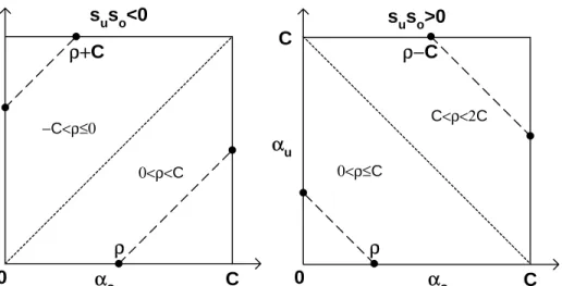
0 αu αo C C ρ ρ+C suso<0 αu αo C C ρ ρ−C suso>0 0 −C<ρ≤0 0<ρ<C 0<ρ≤C C<ρ<2C
Figure 2: An illustration of the boundary for the active variables. The cases corresponding to
suso < 0 and suso > 0 are presented in the left and right part respectively. The dotted line separates the box into two regions for ρ with different values. αo and αu need to be updated jointly along the dashed line within the box, due to the constraints in (12).
Table 1: The basic framework of the SMO algorithm for support vector ordinal regression using explicit threshold constraints.
SMO start at a valid point, α,α∗ and µ, that satisfy (12), find the current Bj
up and Blowj ∀j
Loop do
1. determine theactive threshold J
2. optimize the pair of active variables and the set µa 3. computeBj
up and Blowj ∀j at the new point
while the optimality condition (19) has not been satisfied
Exit returnα, α∗ and b the current point (αold
o , αoldu ) to reach the new point, (αnewo , αnewu ).
It is possible that jo = ju. In this case, named as cross update, more than one equal-ity constraint in (12) is involved in the optimization that may update the variable set µa = {µmin{jo,ju}+1, . . . , µmax{jo,ju}}, a subset of µ. In the case of j
o =ju, named as standard update, only one equality constraint is involved and the variables ofµare kept intact, i.e. µa=∅. These suboptimization problems can be solved analytically, and the detailed formulas for updating are given in the following.
subopti-mization problem: nj i=1 αji +µj = nj+1 i=1 α∗ij+1+µj+1, min{jo, ju} ≤j ≤max{jo, ju}. (20)
Under these constraints the suboptimization problem for αo, αu and µa can be written as
min αo,αu,µa 1 2 j,i j,i (α∗ij−αji)(α∗ij −αj i)K(x j i, xj i)−αo−αu (21)
subject to the bound constraints 0≤αo ≤C, 0≤αu ≤C andµa≥0. The equality constraints (20) can be summarized forαo and αu as a linear constraint αo+sosuαu =αold
o +sosuαoldu =ρ, where so = −1 if io ∈Ijo 0a∪I2jo +1 if io ∈Ijo 0b ∪I jo 4 su = −1 if iu ∈Iju 0a∪Ij u 3 +1 if iu ∈Iju 0b ∪I ju 1 (22)
It is quite straightforward to verify that, for the above optimization problem which is restricted toαo, αu and µa, one can use the same derivations that led to (17) to show that the optimality conditions for the restricted problem is nothing but bjo
low ≤ bjupu. Since we started with this condition being violated, we are guaranteed that the solution of the restricted optimization problem will lead to a strict improvement in the objective function.
To solve the restricted optimization problem, first consider the case of a positive definite kernel matrix. For this case, the unbounded solution can be exactly determined as
αnew o =αoldo +so∆µ αnew u =αoldu −su∆µ µjnew=µjold−dµ∆µ ∀µj ∈µa (23) where dµ= +1 if jo ≤ju −1 if jo > ju (24)
and
∆µ= −f(xo) +f(xu) +so−su
K(xo, xo) +K(xu, xu)−2K(xo, xu), (25) Now we need to check the box bound constraint on αo and αu and the constraint µj ≥ 0. We have to adjust ∆µ towards 0 to draw the out-of-range solution back to the nearest boundary point of the feasible region (see Figure 2, and update variables accordingly as in (23). Note that the cross update allows αo and αu to be associated with the same sample. For the positive semi-definite kernel matrix case, the denominator of (25) can vanish. Still, leaving out the denominator defines the descent direction which needs to be traversed till the boundary is hit, in order to get the optimal solution.
It should be noted that, working with just any violating pair of variables does not automat-ically ensure the convergence of the SMO algorithm. However, since the most violating pair is always chosen, the ideas of Keerthi and Gilbert (2002) can be adapted to prove the convergence of the SMO algorithm.
4
Approach 2: Implicit Constraints on Thresholds
In this section we present a new approach to support vector ordinal regression. Instead of considering only the empirical errors from the samples of adjacent categories to determine a threshold, we allow the samples in all the categories to contribute errors for each threshold. This kind of loss functions was also suggested by Srebro et al. (2005) for collaborative filtering. A very nice property of this approach is that the ordinal inequalities on the thresholds are satisfied automatically at the optimal solution in spite of the fact that such constraints on the thresholds are not explicitly included in the new formulation. We give a proof on this property in the following section.
Figure 3 explains the new definition of slack variables ξ and ξ∗. For a threshold bj, the function values of all the samples from all the lower categories, should be less than the lower margin bj − 1; if that does not hold, then ξkij = w·φ(xki) −(bj −1) is taken as the error associated with the sample xk
samples from the upper categories should be greater than the upper margin bj + 1; otherwise
ξki∗j = (bj + 1)− w ·φ(xki) is the error associated with the sample xki for bj, where k > j. Here, the subscriptkidenotes that the slack variable is associated with thei-th input sample in the k-th category; the superscript j denotes that the slack variable is associated with the lower categories of bj; and the superscript ∗j denotes that the slack variable is associated with the upper categories of bj.
4.1
Primal Problem
By taking all the errors associated with all r−1 thresholds into account, the primal problem can be defined as follows:
min w,b,ξ,ξ∗ 1 2w·w+C r−1 j=1 j k=1 nk i=1 ξkij + r k=j+1 nk i=1 ξki∗j (26) subject to w·φ(xki) −bj ≤ −1 +ξkij , ξkij ≥0, for k= 1, . . . , j and i= 1, . . . , nk; w·φ(xk i) −bj ≥+1−ξki∗j, ξki∗j ≥0, for k=j+ 1, . . . , r and i= 1, . . . , nk; (27)
where j runs over 1, . . . , r−1. Note that there are r−1 inequality constraints for each sample
xk
i (one for each threshold).
To prove the inequalities on the thresholds at the optimal solution, let us consider the situation where w is fixed and only the bj’s are optimized. Note that the ξkij and ξki∗j are automatically determined once the bj are given. To eliminate these variables, let us define, for 1≤k ≤r, Ilow k (b) def = {i∈ {1, . . . , nk}:w·φ(xk i) −b≥ −1}, Ikup(b)def= {i∈ {1, . . . , nk}:w·φ(xki) −b ≤1}.
b2 b1
y=1 y=2 y=3
b2-1 b2+1 b1-1 b1+1 ξ2i∗ 1 f(x) = w φ(x). ξ2i 2 ξ3i∗ 2 ξ3i∗ 1 ξ1i 1
Figure 3: An illustration on the new definition of slack variablesξ and ξ∗ that imposes implicit constraints on the thresholds. All the samples are mapped byw·φ(x)onto the axis of function values. Note the term ξ∗1
3i in this graph.
It is easy to see that bj is optimal iff it minimizes the function
ej(b) = j k=1 i∈Iklow(b) w·φ(xki) −b+ 1+ r k=j+1 i∈Iupk (b) −w·φ(xki)+b+ 1 (28) Let B
j denote the set of all minimizers of ej(b). By convexity, Bj is a closed interval. Given two intervals B1 = [c1, d1] and B2 = [c2, d2], we say B1 ≤B2 if c1 ≤c2 and d1 ≤d2.
Lemma 1. B
1 ≤B2 ≤ · · · ≤Br−1
Proof. The “right side derivative” of ej with respect to b is
gj(b) =−kj=1|Iklow(b)|+rk=j+1|Ikup(b)| (29)
Take any one j and consider B
j = [cj, dj] and Bj+1 = [cj+1, dj+1]. Suppose cj > cj+1. Define
b
j =cj andbj+1 =cj+1. Sincebj+1 is strictly to the left of the intervalBj that minimizesej, we have gj(bj+1)<0. Since bj+1 is a minimizer of ej+1 we also have gj+1(bj+1)≥0. Thus we have
gj+1(bj+1)−gj(bj+1)>0; also, by (29) we get
0< gj+1(bj+1)−gj(bj+1) =−|Ijlow+1(bj+1)| − |I up
j+1(bj+1)|
If the optimal bj are all unique,2 then Lemma 1 implies that theb
j satisfy the natural ordinal ordering. Even when one or more bj’s are non-unique, Lemma 1 says that there exist choices for the bj that obey the natural ordering. The fact that the order preservation comes about automatically is interesting and non-trivial, which differs from the PRank algorithm (Crammer and Singer, 2002) where the order preservation on the thresholds is easily brought in via their update rule.
It is also worth noting that Lemma 1 holds even for an extended problem formulation that allows the use of different costs (different C values) for different misclassifications (classk mis-classified as classj can have aCkj). In applications such as collaborative filtering such a problem formulation can be very appropriate; for example, an A rated movie that is misrated as D may need to be penalized much more than if a B rated movie is misrated as D. Shashua and Levin’s formulation and its extension given in section 2 of this paper do not precisely support such a differential cost structure. This is another good reason in support of the implicit problem formulation of the current section.
4.2
Dual Problem
Let αjki ≥0, γjki ≥ 0, α∗kij ≥0 and γki∗j ≥ 0 be the Lagrangian multipliers for the inequalities in (27). Using ideas parallel to those in section 2.1 we can show that the dual of (26)–(27) is the following maximization problem that involves only the multipliersα and α∗:
max α,α∗− 1 2 k,i k,i k−1 j=1 α∗kij − r−1 j=k αjki k−1 j=1 α∗kji− r−1 j=k αjki K(xki, xki) + k,i k−1 j=1 α∗kij + r−1 j=k αjki (30) subject to j k=1 nk i=1 αkij = r k=j+1 nk i=1 α∗kij ∀j 0≤αkij ≤C ∀j and k ≤j 0≤αki∗j ≤C ∀j and k > j. (31)
2If, in the primal problem, we regularize theb
j’s as well (i.e., include the extra cost termjb2j/2) then the
The dual problem (30)–(31) is a convex quadratic programming problem. The size of the optimization problem is (r−1)n where n = rk=1nk is the total number of training samples. The discriminant function value for a new input vectorx is
f(x) = w·φ(x)= k,i k−1 j=1 α∗kij − r−1 j=k αjki K(xki, x). (32)
The predictive ordinal decision function is given by arg min
i {i:f(x)< bi}.
4.3
Optimality Conditions for the Dual
The Lagrangian for the dual problem is
Ld= 1 2 k,i k,i k−1 j=1α ∗j ki − r−1 j=kα j ki k −1 j=1 α ∗j ki − r−1 j=kα j ki K(xk i, xk i) −k,ik−1 j=1α∗kij+ r−1 j=kαjki +rj=1−1βj(jk=1ni=1k αjki−rk=j+1ni=1k α∗kij) −r−1 j=1 j k=1 nk i=1ηjkiαjki− r−1 j=1 r k=j+1 nk i=1ηki∗jα∗kij −r−1 j=1 j k=1 nk i=1π j ki(C−α j ki)− r−1 j=1 r k=j+1 nk i=1π ∗j ki(C−α ∗j ki) (33)
where the Lagrangian multipliers ηjki, η∗kij, πjki and πki∗j are non-negative, while βj can take any value. The KKT conditions associated with βj can be given as follows:
∂Ld ∂αjki =−f(x k i)−1−ηkij +π j ki+βj = 0, πkij ≥0, ηjki ≥0, πkij (C−αkij ) = 0, ηjkiαjki = 0,for k ≤j and ∀i; ∂Ld ∂α∗kij =f(xk i)−1−ηki∗j +π ∗j ki −βj = 0, πki∗j ≥0, ηki∗j ≥0, πki∗j(C−αki∗j) = 0, ηki∗jαki∗j = 0,fork > j and ∀i; (34)
where f(x) is as defined in (32). The conditions in (34) can be regrouped into the following six cases: case 1 : αjki = 0 f(xki) + 1 ≤βj case 2 : 0< αjki < C f(xk i) + 1 =βj case 3 : αjki =C f(xk i) + 1 ≥βj case 4 : α∗kij = 0 f(xki)−1≥βj case 5 : 0< α∗kij < C f(xk i)−1 = βj case 6 : α∗kij =C f(xk i)−1≤βj (35)
We can classify any variable into one of the following six sets:
I0ja =i∈ {1, . . . , nk}: 0< αjki < C, k≤j I0jb =i∈ {1, . . . , nk}: 0< α∗j ki < C, k > j I1j =i∈ {1, . . . , nk}:α∗j ki = 0, k > j I2j =i∈ {1, . . . , nk}:αjki = 0, k≤j I3j =i∈ {1, . . . , nk}:αj ki =C, k≤j I4j =i∈ {1, . . . , nk}:α∗j ki =C, k > j (36) Let us denote I0j =I0ja∪I0jb, Ij
up =I0j∪I1j∪I3j and Ilowj =I0j∪I2j∪I4j. We further define Fupj on the set Iupj as Fupj = f(xk i) + 1 if i∈I0ja∪I3j f(xk i)−1 if i∈I0jb∪I1j (37)
and Flowj on the set Ilowj as
Flowj = f(xk i) + 1 if i∈I0ja∪I2j f(xk i)−1 if i∈I0jb∪I4j (38)
Then the optimality conditions can be simplified as
which can be compactly written as
bjlow ≤βj ≤bjup (40) where bj
up = min{Fupj : i ∈ Iupj } and bjlow = max{Flowj :i ∈ Ilowj }. By introducing the tolerance parameter τ >0, we get the approximate stopping condition
max{bjlow−bjup:j = 1, . . . , r−1} ≤τ (41)
4.4
SMO Algorithm
The ideas for adapting SMO to (30)–(31) are similar to those in section 3. The resulting suboptimization problem is analogous to the case of standard update in section 3 where only one of the equality constraints from (31) is involved.
The index ofactive thresholdcan be determined asJ = arg maxj{bjlow−bj
up}, and then the two multipliers associated withbJ
low and bJup are used as the active variables for the suboptimization problem. Let us denote these active variables as αo andαu, the corresponding indices asio and
iu, and the corresponding samples as xo and xu respectively. The suboptimization problem of (30)–(31) for αo and αu becomes
min αo,αu S(αo, αu) = 1 2 k,i k,i k−1 j=1 α∗kij− r−1 j=k αjki k−1 j=1 α∗kji − r−1 j=k αjki K(xki, xik)−αo−αu (42)
subject to the bound constraints 0 ≤ αo ≤ C, 0 ≤ αu ≤ C, and the linear constraint αo+
sosuαu =ρ, where so= −1 if io ∈IJ 0a∪I2J +1 if io ∈I0Jb∪I4J su = −1 if iu ∈IJ 0a∪I3J +1 if iu ∈IJ 0b ∪I1J (43)
The index sets used above are as defined in (36). This is analogous to the case of standard update in section 3 where only one of the equality constraints from (12) is involved. Due to the linear constraint between αo and αu, the unbounded solution to (42) can be exactly determined
as
αnewo =αoldo +so −f(xo) +f(xu) +so−su
K(xo, xo) +K(xu, xu)−2K(xo, xu) (44) wheref(x) is as defined in (32). Next, we check ifαnew
o satisfies all the box constraints (see Figure 2 for an illustration) and, if it doesn’t satisfy them, then we draw it back to the nearest boundary point of the box. Using the final value of αnew
o , αu can be updated as αnewu = suso(ρ−αonew) where ρ=αold
o +sosuαoldu .
5
Numerical Experiments
We have implemented the two SMO algorithms for the ordinal regression formulations with explicit constraints (EXC) and implicit constraints (IMC),3 along with the algorithm of Shashua and Levin (2003) for comparison purpose. The function caching technique and the double-loop scheme proposed by Keerthi et al. (2001) have been incorporated in the implementation for efficiency. We begin this section with a simple dataset to illustrate the typical behavior of the three algorithms, and then empirically study the scaling properties of our algorithms. Then we compare the generalization performance of our algorithms against standard support vector regression on eight benchmark datasets for ordinal regression. The following Gaussian kernel was used in these experiments:
K(x, x) = exp −κ 2 d ς=1(xς−xς)2 (45)
where κ >0 and xς denotes the ς-th element of the input vector x. The tolerance parameter τ
was set to 0.001 for all the algorithms. We have utilized two evaluation metrics which quantify the accuracy of predicted ordinal scales {yˆ1, . . . ,yˆt} with respect to true targets {y1, . . . , yt}:
a) Mean absolute error is the average deviation of the prediction from the true target, i.e. 1
t
t
i=1|yˆi−yi|, in which we treat the ordinal scales as consecutive integers;
b) Mean zero-one error is simply the fraction of incorrect predictions on individual samples. 3The source code of the two algorithms written in ANSI C can be found at
450 500 550 600 1 2 3 4 5
Grade in probability course
Sat−math score Shashua and Levin’s formulation
b 1=0.01 b 2=−0.15 450 500 550 600 1 2 3 4 5
Grade in probability course
Sat−math score with implicit constraints
b 1=−0.51 b 2=0.74 450 500 550 600 1 2 3 4 5
Grade in probability course
Sat−math score with explicit constraints
b
1=b2=−0.07
(a) (b) (c)
Figure 4: The training results of the three algorithms using a Gaussian kernel on the grading dataset. The discriminant function values are presented as contour graphs indexed by the two thresholds. The circles denote the students with grade D, the dots denote grade C, and the squares denote grade B.
5.1
Grading Dataset
The grading dataset was used in chapter 4 of Johnson and Albert (1999) as an example of the ordinal regression problem.4 There are 30 samples of students’ score. The “sat-math score” and “grade in prerequisite probability course” of these students are used as input features, and their final grades are taken as the targets. In our experiments, the six students with final grade A or E were not used, and the feature associated with the “grade in prerequisite probability course” was treated as a continuous variable though it had an ordinal scale. In Figure 4 we present the solution obtained by the three algorithms using the Gaussian kernel (45) with κ= 0.5 and the regularization factor value of C = 1. In this particular setting, the solution to Shashua and Levin (2003)’s formulation has disordered thresholds b2 < b1 as shown in Figure 4 (left plot); the formulation with explicit constraints corrects this disorder and yields equal values for the two thresholds as shown in Figure 4 (middle plot).
5.2
Scaling
In this experiment, we empirically studied how the two SMO algorithms scale with respect to training data size and the number of ordinal scales in the target. The California Housing dataset
100 500 1000 2000 5000
10−2
100
102
104
Training data size
CPU time in seconds
5 ordinal scales in the target implicit constraints
explicit constraints support vector regression
100 500 1000 2000 5000
10−2
100
102
104
Training data size
CPU time in seconds
10 ordinal scales in the target implicit constraints
explicit constraints support vector regression
slope ≈ 2.13 slope ≈ 2.18 slope ≈ 2.43 slope ≈ 2.13 slope ≈ 2.33 slope ≈ 2.39
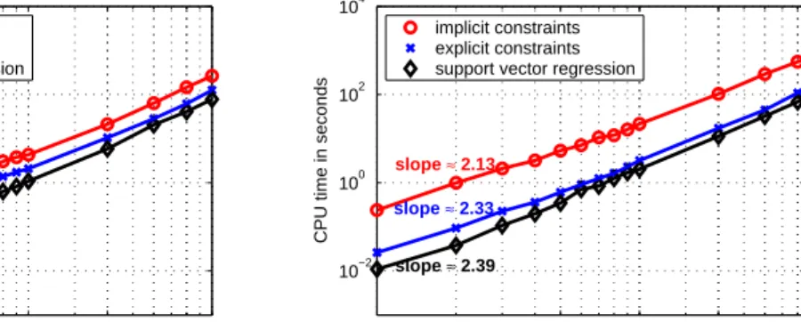
Figure 5: Plots of CPU time versus training data size on log−log scale, indexed by the estimated slopes respectively. We used the Gaussian kernel withκ = 1 and the regularization factor value of C = 100 in the experiment.
was used in the scaling experiments.5 Twenty-eight training datasets with sizes ranging from 100 to 5,000 were generated by random selection from the original dataset. The continuous target variable of the California Housing data was discretized to ordinal scale by using 5 or 10 equal-frequency bins. The standard support vector regression (SVR) was used as a baseline, in which the ordinal targets were treated as continuous values and =0.1. These datasets were trained by the three algorithms using a Gaussian kernel with κ=1 and a regularization factor value of C=100. Figure 5 gives plots of the computational costs of the three algorithms as functions of the problem size, for the two cases of 5 and 10 target bins. Our algorithms scale well with scaling exponents between 2.13 and 2.33, while the scaling exponent of SVR is about 2.40 in this case. This near-quadratic property in scaling comes from the sparseness property of SVMs, i.e., non-support vectors affect the computational cost only mildly. The EXC and IMC algorithms cost more than the SVR approach due to the larger problem size. For large sizes, the cost of EXC is only about 2 times that of SVR in this case. As expected, we also noticed that the computational cost of IMC is dependent on r, the number of ordinal scales in the target. The cost for 10 ranks is observed to be roughly 5 times that for 5 ranks, whereas the cost of EXC is nearly the same for the two cases. These observations are consistent with the size of the optimization problems. The problem size of IMC is (r −1)n (which is heavily influenced byr) while the problem size of EXC is about 2n+r (which largely depends on n only since we usually haven r). This factor of efficiency can be a key advantage for the EXC formulation.
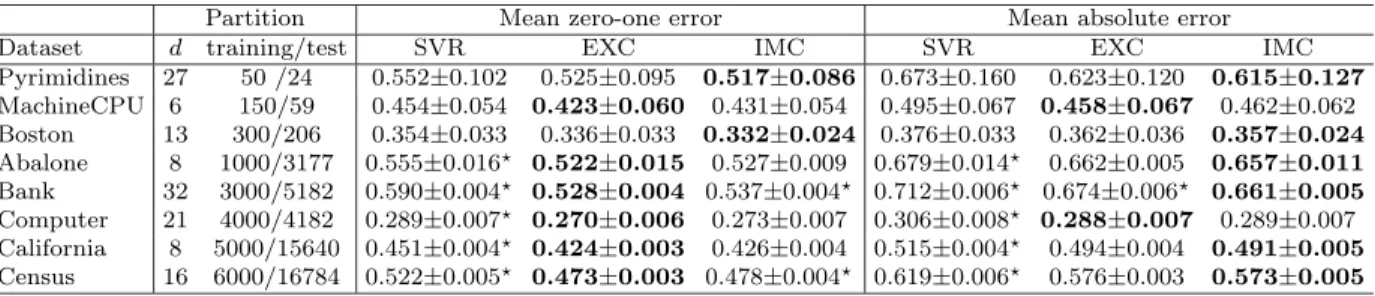
Table 2: Test results of the three algorithms using a Gaussian kernel. The targets of these benchmark datasets were discretized into 5 equal-frequency bins. ddenotes the input dimension and “training/test” denotes the partition size. The results are the averages over 20 trials, along with the standard deviation. We use bold face to indicate the cases in which the average value is the lowest among the results of the three algorithms. The symbols are used to indicate the cases significantly worse than the winning entry; A p-value threshold of 0.01 in Wilcoxon rank sum test was used to decide this.
Partition Mean zero-one error Mean absolute error
Dataset d training/test SVR EXC IMC SVR EXC IMC
Pyrimidines 27 50 /24 0.552±0.102 0.525±0.095 0.517±0.086 0.673±0.160 0.623±0.120 0.615±0.127 MachineCPU 6 150/59 0.454±0.054 0.423±0.060 0.431±0.054 0.495±0.067 0.458±0.067 0.462±0.062 Boston 13 300/206 0.354±0.033 0.336±0.033 0.332±0.024 0.376±0.033 0.362±0.036 0.357±0.024 Abalone 8 1000/3177 0.555±0.016 0.522±0.015 0.527±0.009 0.679±0.014 0.662±0.005 0.657±0.011 Bank 32 3000/5182 0.590±0.004 0.528±0.004 0.537±0.004 0.712±0.006 0.674±0.006 0.661±0.005 Computer 21 4000/4182 0.289±0.007 0.270±0.006 0.273±0.007 0.306±0.008 0.288±0.007 0.289±0.007 California 8 5000/15640 0.451±0.004 0.424±0.003 0.426±0.004 0.515±0.004 0.494±0.004 0.491±0.005 Census 16 6000/16784 0.522±0.005 0.473±0.003 0.478±0.004 0.619±0.006 0.576±0.003 0.573±0.005 Table 3: Test results of the four algorithms using a Gaussian kernel. The partition sizes of these benchmark datasets were same as that in Table 2, but the targets were discretized by 10 equal-frequency bins. The results are the averages over 20 trials, along with the standard deviation. We use bold face to indicate the lowest average value among the results of the four algorithms. The symbols are used to indicate the cases significantly worse than the winning entry; A p-value threshold of 0.01 in Wilcoxon rank sum test was used to decide this.
Mean zero-one error Mean absolute error
Dataset SVR SLA EXC IMC SVR SLA EXC IMC
Pyrimidines 0.777±0.068 0.756±0.073 0.752±0.063 0.719±0.066 1.404±0.184 1.400±0.255 1.331±0.193 1.294±0.204 Machinecpu 0.693±0.0560.643±0.057 0.661±0.056 0.655±0.045 1.048±0.141 1.002±0.121 0.986±0.127 0.990±0.115 Boston 0.589±0.0250.561±0.023 0.569±0.025 0.561±0.026 0.785±0.052 0.765±0.057 0.773±0.049 0.747±0.049 Abalone 0.758±0.0170.739±0.008 0.736±0.011 0.732±0.0071.407±0.0211.389±0.0271.391±0.0211.361±0.013 Bank 0.786±0.0040.759±0.0050.744±0.0050.751±0.0051.471±0.0101.414±0.0121.512±0.0171.393±0.011 Computer 0.494±0.006 0.462±0.006 0.462±0.0050.473±0.0050.632±0.011 0.597±0.010 0.602±0.009 0.596±0.008 California 0.677±0.0030.640±0.003 0.640±0.003 0.639±0.003 1.070±0.0081.068±0.0061.068±0.0051.008±0.005 Census 0.735±0.0040.699±0.002 0.699±0.0020.705±0.0021.283±0.0091.271±0.0071.270±0.0071.205±0.007
5.3
Benchmark datasets
Next, we compared the generalization performance of the two approaches against the naive approach of using standard support vector regression (SVR) and the method (SLA) of Shashua and Levin (2003). We collected eight benchmark datasets that were used for metric regression problems.6 The target values were discretized into ordinal quantities using equal-frequency binning. For each dataset, we generated two versions by discretizing the target values into five or ten ordinal scales respectively. We randomly partitioned each dataset into training/test splits as specified in Table 2. The partitioning was repeated 20 times independently. The input vectors
were normalized to zero mean and unit variance, coordinate-wise. The Gaussian kernel (45) was used for all the algorithms. 5-fold cross validation was used to determine the optimal values of model parameters (the Gaussian kernel parameterκand the regularization factorC) involved in the problem formulations, and the test error was obtained using the optimal model parameters for each formulation. The initial search was done on a 7×7 coarse grid linearly spaced in the region {(log10C,log10κ)| −3 ≤ log10C ≤ 3,−3 ≤ log10κ ≤ 3}, followed by a fine search on a 9×9 uniform grid linearly spaced by 0.2 in the (log10C,log10κ) space. The ordinal targets were treated as continuous values in standard SVR, and the predictions for test cases were rounded to the nearest ordinal scale. The insensitive zone parameter, of SVR was fixed at 0.1. The test results of these algorithms are recorded in Table 2 and 3. It is very clear that the generalization capabilities of the three ordinal regression algorithms are better than that of the approach of SVR. The performance of Shashua and Levin’s method is similar to our EXC approach, as expected, since the two formulations are pretty much the same. Our ordinal algorithms are comparable on the mean zero-one error, but the results also show the IMC algorithm yields much more stable results on mean absolute error than the EXC algorithm.7 From the view of the formulations, EXC only considers the extremely worst samples between successive ranks, whereas IMC takes all the samples into account. Thus the outliers may affect the results of EXC significantly, while the results of IMC are relatively more stable in both validation and test.
5.4
Information Retrieval
Ranking learning arises frequently in information retrieval. Hersh et al. (1994) generated the OHSUMED dataset,8 which consists of 348566 references and 106 queries with their respective ranked results. The relevance level of the references with respect to the given textual query were assessed by human experts, using a three rank scale: definitely, possibly, or not relevant. In our experiments, we used the results of query 1 which contain 107 assessed references (19 defi-nitely relevant, 14 possibly relevant and 74 irrelevant) taken from the whole database. In order
7As a plausible argument, ξj
i +ξi∗j+1 in (2) of EXC is an upper bound on the zero-one error of the i-th
example, while, in (18) of IMC,jk=1ξkij +rk=j+1ξki∗j is an upper bound on the absolute error. Note that, in all the examples we use consecutive integers to represent the ordinal scales.
to apply our algorithms the bag-of-words representation was used to translate these reference documents into vectors. We computed, for all documents the vector of “term frequencies”(TF) components scaled by “inverse document frequencies”(IDF). The TFIDF is a weighted scheme for the bag-of-words representation which gives higher weights to terms which occur very rarely in all documents. We used the “rainbow” software released by McCallum (1998) to scan the title and abstract of these references for the bag-of-words representation. In the preprocessing, we skipped the terms in the “stoplist”,9 and restricted ourselves to terms that appear in at least 3 of the 107 documents. This results in 462 distinct terms. So each document is represented by its TFIDF vector with 462 elements. To account for different document lengths, we normalized the length of each document vector to unity (Joachims, 1998).
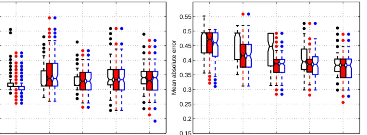
We randomly selected a subset of the 107 references (with size chosen from {20,30, . . . ,60}) for training and then tested on the remaining references. For each size, the random selection was repeated 100 times. The generalization performance of the two support vector algorithms for ordinal regression were compared against the naive approach of using support vector regression. The linear kernelK(xi, xj) = xi·xjwas employed for all the three algorithms. The test results of the three algorithms are presented as boxplots in Figure 6. In this case, the zero-one error rates are almost at same level, but the naive approach yields much worse absolute error rate than the two ordinal SVM algorithms.
5.5
Collaborative Filtering
Collaborative filtering is to predict a person’s rating on new items given the person’s past ratings on similar items and the ratings of other people on all the items (including the new item). This is a typical ordinal regression problem (Shashua and Levin, 2003), since the ratings given by the users are usually discrete and ordered. We carried out ordinal regression on a subset of the EachMovie data.10 The ratings given by the user with ID number 52647 on 449 movies were used as the targets, in which the numbers of zero-to-five stars are 40, 20, 57, 113, 145 and 74
9The “stoplist” is the SMART systems’ list of 524 common words, like “the” and “of”.
10The Compaq System Research Center ran the EachMovie service for 18 months. 72916 users entered a total
20 30 40 50 60 0.15 0.2 0.25 0.3 0.35 0.4 0.45 0.5 0.55
Mean zero−one error
Training data size
20 30 40 50 60 0.15 0.2 0.25 0.3 0.35 0.4 0.45 0.5 0.55
Mean absolute error
Training data size
Figure 6: The test results of the three algorithms on the subset of the OHSUMED data relating to query 1, over 100 trials. The grouped boxes represent the results of SVR (left), EXC (middle) and IMC (right) at different training data sizes. The notched-boxes have lines at the lower quartile, median, and upper quartile values. The whiskers are lines extending from each end of the box to the most extreme data value within 1.5·IQR(Interquartile Range) of the box. Outliers are data with values beyond the ends of the whiskers, which are displayed by dots. The left graph gives mean zero-one error and the right graph gives mean absolute error.
respectively. We selected 1500 users who contributed the most ratings on these 449 movies as the input features, i.e. the ratings given by the 1500 users on each movie were used to form the input vector. In the 449×1500 input matrix, about 40% elements were observed. We randomly selected a subset (with size taking values from {50,100, . . . ,300}) of the 449 movies for training, and then tested on the remaining movies. For each size, the random selection was carried out 50 times.
Pearson correlation coefficient (a particular dot product between normalized rating vectors) is the most popular correlation measure in collaborative filtering (Basilico and Hofmann, 2004). Applied to the movies, we can define the so-called z-scores as z(v, u) = r(v,uσ)(−v)µ(v), where u
indexes users, v indexes movies, and r(v, u) is the rating on the movie v given by the user u.
µ(v) andσ(v) are the movie-specific mean and standard deviation respectively. This correlation coefficient, defined as
K(v, v) = u
z(v, u)z(v, u) (46)
whereu denotes summing over all the users, was used as the kernel function in our experiments for the three algorithms. As not all ratings are observed in the input vectors, we use mean imputation as a reasonable strategy to deal with missing values. Thus, unobserved values are
50 100 150 200 250 300 0.5 0.55 0.6 0.65 0.7 0.75 0.8
Mean zero−one error
Training data size
50 100 150 200 250 300 0.7 0.75 0.8 0.85 0.9 0.95 1 1.05 1.1
Mean absolute error
Training data size
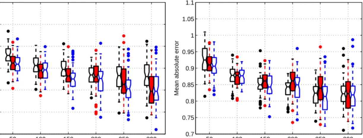
Figure 7: The test results of the three algorithms on a subset of EachMovie data, averaged over 50 trials. The grouped boxes represent the results of SVR (left), EXC (middle) and IMC (right) at different training data sizes. The left graph gives mean zero-one error and the right graph gives mean absolute error.
identified with the mean value, which means that their corresponding z-score is zero.
The test results are presented as boxplots in Figure 7. In this application, the naive approach yields much worse zero-one error rate than the two ordinal SVM algorithms and IMC performs better than EXC in many cases.
6
Conclusion
In this paper we proposed two new approaches to support vector ordinal regression that deter-mine r−1 parallel discriminant hyperplanes for the r ranks by using r −1 thresholds. The ordinal inequality constraints on the thresholds are imposed explicitly in the first approach and implicitly in the second one. The problem size of the two approaches is linear in the number of training samples. We also designed SMO algorithms that scale only about quadratically with the problem size. The results of numerical experiments verified that the generalization capabilities of these approaches are much better than the naive approach of applying standard regression.