Low-Rank Approximation and Difusion Maps

(1)

UNIVERSIDAD AUT ´

ONOMA DE MADRID

ESCUELA POLIT´

ECNICA SUPERIOR

TRABAJO FIN DE M ´ASTER

Low-Rank Approximation and Diffusion Maps

Máster Universitario en Investigación e Innovación en TIC (i2_-TIC)

Autor: DORADO ALFARO, Sara

Tutor: DORRONSORO IBERO, Jos´

e Ram´

on

Cotutor: FERN ´

ANDEZ PASCUAL, ´

Angela

Departamento de Ingenier´ıa Inform´atica

(2)

(3)

List of Figures

2.1.1 Helix embedding via PCA . . . 8

2.3.1 Influence of α on an helix example . . . 17

2.4.1 Spectral Clustering in the noisy moons dataset . . . 19

3.3.1 Standard Multilayer Perceptron with two hidden layers. . . 27

3.3.2 Autoencoder . . . 28

4.2.1 Replication of the Helix dataset embedding from [1] . . . 36

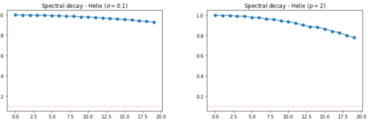
4.2.2 Spectral decay of the Helix for different values of σ . . . 37

4.2.3 Embeddings for the Helix dataset for fixed t= 1 and different values of σ . 37 4.2.4 Spectral decay of the Helix dataset fort= 1 . . . 38

4.2.5 Spectral decay of the Helix for different values of t . . . 38

4.2.6 Embedding and spectral decay for the Helix dataset . . . 39

4.2.7 Boxplots of the Red Wine dataset . . . 40

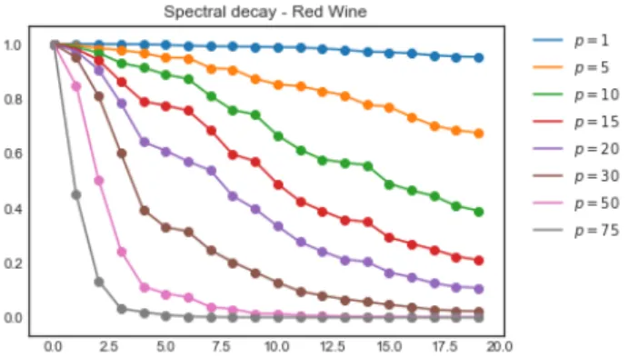
4.2.8 Spectral decay of the Red Wine dataset for different values ofσ and t= 1 . 41 4.2.9 Embedding computed for the Red Wine dataset for fixed t= 1 . . . 41

4.2.10Spectral decay of the Red Wine dataset for different values oft . . . 42

4.2.11Embedding for the Red Wine dataset. . . 42

4.2.12Spectral decay of the Vowel dataset for different values of σ and t= 1 . . . 43

4.2.13Embeddings computed for the Vowel dataset for fixed t= 1 . . . 43

4.2.14Spectral decay of the Vowel dataset for different values of tand p= 1 . . . 44

4.2.15Embedding for the Vowel dataset . . . 44 vii

(8)

viii List of Figures

4.3.1 Graphical representation of the Nystr¨om method to extend the embedding

to OOS examples. . . 45

4.3.2 OOS extension of the Helix dataset with Nystr¨om’s method and reconstruc-tion error . . . 46

4.3.3 OOS extension with Nystr¨om’s method of the Red Wine dataset . . . 47

4.3.4 Reconstruction error via Nystr¨om for the Red Wine dataset . . . 47

4.3.5 OOS extension with Nystr¨om’s method of the Vowel dataset . . . 48

4.3.6 Reconstruction error via Nystr¨om for the Vowel dataset . . . 48

4.4.1 Grid search for µ . . . 49

4.4.2 Diffusion Nets applied to the Helix dataset . . . 50

4.4.3 Diffusion Nets applied to the Red Wine dataset . . . 51

(9)

List of Tables

4.1.1 Datasets description. . . 34 4.2.1 Distribution of the targets in the Red Wine dataset. . . 40

(10)

(11)

List of Algorithms

1 Encoder . . . 29 2 Decoder . . . 31 3 Autoencoder . . . 31

(12)

(13)

Resumen

La teor´ıa de la reducción de la dimensionalidad es fundamental para muchos problemas de Aprendizaje Automático. Existen multitud de enfoques, pero este trabajo se centrará en los métodos de aprendizaje de variedades. El punto de partida es asumir que los datos viven en una variedad de dimensión menor que la de partida para lograr entender el fenómeno subyacente que los ha generado. Dentro de este campo, es de especial interés, debido a su fuerte base matemática, el algoritmo conocido como Mapas de Difusión, objeto principal de este trabajo.

Primero realizaremos un estudio de los Mapas de Difusión as´ı como de la teor´ıa ma-temática necesaria para su correcta comprensión, estudiando conceptos como los Grafos de Semejanza y sus Laplacianos y la Distancia de Difusión. El principal inconveniente de los Mapas de Difusión, as´ı como de otros algoritmos espectrales, es que requiere la diagonali-zación de una matriz cuadrada cuya dimensión es el número de ejemplos. Por lo tanto, su coste computacional es O(N3), donde N se refiere al número de ejemplos. Es por ello que uno de los objetivos de este trabajo es calcular una aproximación de rango bajo para los Mapas de Difusión mediante el método de Nyström. Además, para evaluar la calidad de la aproximación, propondremos una métrica que se basa en el error de reconstrucción de la matriz de difusión. Por otro lado, existe otro problema cuando se quiere dar la proyección de un ejemplo que no está en la muestra inicial utilizada para el cálculo de la transforma-ción. Es necesario rehacer el análisis espectral de la matriz, lo que es especialmente cr´ıtico si las aplicaciones tienen restricciones de funcionamiento en tiempo real. En este trabajo también analizaremos dos propuestas para paliar este coste: aprender el mapeo por medio de redes neuronales para regresión (Redes de Difusión), pudiendo as´ı calcular la proyección para un nuevo ejemplo, y calcular una extensión de la transformación para un nuevo punto con el método de Nyström.

A la hora de mostrar los resultados se van a utilizar tres conjuntos de datos, uno de los cuales será sintético. Para todos ellos, se calculará la transformación a un espacio de menor dimensión por medio de Mapas de Difusión con el objetivo de extender los mismos a ejemplos fuera de muestra y evaluar la aproximación de rango bajo conseguida por el método de Nyström. Además, se calcularán extensiones para patrones fuera de muestra y se compararán los resultados obtenidos, tanto por las Redes de Difusión como por el método de Nyström, de forma visual.

En resumen, en cuanto a la calidad de la aproximación de rango bajo veremos que, como cabr´ıa esperar, incrementar el número de ejemplos en el conjunto de entrenamiento conlleva una reducción del error de reconstrucción de la matriz de difusión. En cuanto al funcionamiento de los métodos para extender el mapeo a ejemplos fuera de muestra, obser-varemos que tanto el método de Nyström como las Redes de Difusión obtienen resultados visualmente similares, proyectando ejemplos de la misma clase en las mismas regiones del espacio.

Este trabajo da lugar a nuevas l´ıneas de investigaci´on, ya que como trabajo futuro es de especial inter´es, entre otros, conseguir comparar la calidad de las extensiones para ejemplos fuera de muestra.

(14)

(15)

Abstract

The theory of dimensionality reduction is fundamental for many problems of Machine Learning. There are many approaches, but this work will focus on the methods of Manifold Learning. The starting point is to assume that data live in a manifold of smaller dimension than the starting one in order to understand the underlying phenomenon that has generated them. Within this field, it is of special interest, due to its strong mathematical foundation, the algorithm known as Diffusion Maps, the main object of this work.

First we will study the theory of Diffusion Maps, as well as the mathematical theory necessary for its correct understanding, studying concepts such as Similarity Graphs and their Laplacians, and the Diffusion Distance. The main drawback of Diffusion Maps, as well as other spectral algorithms, is that they require the diagonalization of a square matrix whose dimension is the number of examples. Therefore, its computational cost is O(N3), where N refers to the number of examples. Because of that, one of the main objectives of this work is to compute a low-rank approximation for Diffusion Maps using Nystr¨om’s method. In addition, in order to evaluate the quality of the approach, we will propose a metric that is based on the reconstruction error of the diffusion matrix. On the other hand, there is another problem when giving the embedding for examples that were not in the initial sample used to compute the embedding. It is necessary to redo the spectral analysis of the matrix, which is especially critical if the applications have operating restrictions in real time. In this work we will also analyze two proposals to allevaite this cost: to learn the embedding by means of neural networks for regression (Diffusion Nets), being able to compute the embedding for a new example, and to compute an extension of the embedding with Nystr¨om’s method.

Regarding the results, three datasets will be used, one of which will be synthetic. For all of them, we will compute the embedding via Diffusion Maps with the objective of extending it to out-of-sample (OOS) examples and to evaluate the low range approximation achieved by Nystr¨om’s method. In addition, extensions for OOS patterns will be computed via Diffusion Nets and Nystr¨om’s method.

To sum up, regarding the low-rank approximation quality we will see that increasing the number of examples in the training set entails a reduction in the reconstruction error of the diffusion matrix, as we could expect. Regarding OOS extensions, we will observe that both, Nystr¨om’s method and Diffusion Nets, obtain visually similar results, embedding examples of the same class in the same regions of space.

This work gives rise to new lines of research, since as future work it is of special interest, among others, to be able to compare the quality of the extensions for OOS examples.

(16)

(17)

Acknowledgements

En primer lugar quiero agradecer a José Ramón Dorronsoro Ibero y a Ángela Fernández Pascual haber sido unos tutores excepcionales. Gracias por los conocimientos, la com-prensión y el tiempo dedicado. Nada de esto habr´ıa sido posible sin vosotros. Gracias también a Carlos Mar´ıa Alaiz Gud´ın y a Alejandro Catalina Feliú por haberme acompañado en algunas de las reuniones semanales, teniendo paciencia para escucharme y corregirme.

Gracias a la Cátedra UAM-IIC de Ciencia de Datos y Aprendizaje Automático por la ayuda para máster concedida, que me ha permitido dedicarme a tiempo completo a mis estudios. Gracias al equipo docente de la Escuela Politécnica Superior y de la Facultad de Ciencias por haberme enseñado todo lo posible, siempre estando dispuestos a concertar tutor´ıas y a aportar ideas.

Un enorme gracias a mi familia. Gracias mamá, por ayudarme cada d´ıa y por esforzarte tanto. Gracias papá, por todos los consejos y por enseñarme que tenemos seis sentidos, incluyendo el sentido común. Y gracias a mi hermano Sergio, por las charlas de futuro y los ratos juntos. Son lo mejor de cada d´ıa. Gracias abuelos, t´ıos y primos por vuestro apoyo y cariño incondicional.

A todos mis compañeros de aventuras estos últimos años. A pesar de los momentos duros, me llevo grandes recuerdos y amigos. En especial, gracias a Carlos por haberme acompañado y ayudado este último año. Y gracias a mis compañeras de deporte, las chicas del Sanfer Senior, porque me habéis dado una v´ıa de escape siempre que la he necesitado. Teneros es genial.

(18)

(19)

Chapter 1

Introduction

1.1 Motivation

In the context of Artificial Intelligence and in the era of Big Data, dimensionality reduction plays a central role. By reducing the number of variables or features of a given problem we do not only achieve more efficiency, but many times we obtain a higher degree of accuracy. Methods of dimensionality reduction, both in classification and regression problems, try to change the representation of the original data by embedding it into a space of lower dimension in which a large part of the data information is retained.

In this work, we will study methods that suppose data lie in a manifold, a field known as manifold learning [2]. These methods have several applications, starting from data visualization to clustering [3]. Because of their good performance, spectral algorithms are very popular among the existing literature. On the one hand, we have the Laplacian Eigenmaps algorithm [4], which gives foundation to the algorithm of Spectral Clustering [5] and has been exhaustively studied. On the other hand, we find a more general technique, which are Diffusion Maps [6], the method that this work focuses on. This algorithm is specially interesting due to its strong mathematical foundation, which lies on the fields of similarity graphs and random walks. Diffusion Maps have a clear advantage over other manifold learning methods: they embed the data into a space in which the standard distance, that is the euclidean distance, approximates the Diffusion Distance in the original space, a robust measure.

The main disadvantage of Diffusion Maps is its computational complexity. In order to give the embedding, we need to compute the eigenvalues and eigenvectors of a square matrix of dimension the number of examples. The first problem of this is that we may not be able to compute the Diffusion Map of a huge dataset. The second problem comes when we want to compute the embedding of new examples, which are known as out-of-sample examples. With the arrival of a new pattern, it is necessary to recalculate the eigenvectors and eigenvalues of a similarity matrix, whose size is, again, the number of examples.

Aiming to solve these problems, we can find several proposals in the literature. One of them is trying to compute a low-rank approximation for the Diffusion Map [4]. That is, to compute the eigenvalues and eigenvectors of the similarity matrix of a small sample and, then, try to extend it to other patterns, which are the out-of-sample patterns. In this

(20)

2 Chapter 1. Introduction

sense, we can incorporate Nytr¨om’s method [7] to Diffusion Maps.

Other approach would be to compute the embedding for a given subset and learn it via any Machine Learning method. This could be, for example, neural networks for regression (the embedding is continuous) in which the target is the embedding we want to extend. This was introduced in [1] under the name of Diffusion Nets.

Thus, the motivation of this work is to review the current state-of-the-art of Diffusion Maps and present the mathematical theory necessary to reach a good understanding of this field. Apart from this review, we will also experiment with different datasets to measure the low-rank approximation quality reached by Nystr¨om’s encoding when applied to Diffusion Maps. In addition, we will compare the results obtained when trying to extend the embedding to out-of-sample examples via any of the previously mentioned approaches: Nystr¨om’s encoding and Diffusion Nets.

1.2 Objectives

The main objective of this work is to introduce a research line focused around low-rank approximation and out-of-sample extension in Diffusion Maps. With this general purpose, this work is focused on the following topics:

• To study and understand the mathematical background of Diffusion Maps.

• To study the theory of Similarity Graphs and Laplacians.

• To study the Nystr¨om’s method and its integration with Diffusion Maps.

• To study Diffusion Nets.

• To implement these concepts and methods and test them in synthetic and real datasets, comparing its performance to extract some conclusions.

1.3 Structure

In this context, this work is structured around three main chapters:

1. Manifold learning and Difussion Maps, where we introduce and develop the necessary mathematical background and the algorithm of Diffusion Maps. We intro-duce Principal Component Analysis, giving an example of the necessity of non-linear methods for dimensionality reduction. This chapter also contains the theory of Sim-ilarity Graphs and Laplacians and the algorithm of Laplacian Eigenmaps.

2. Out-of-sample extension, where different approaches to extend the embedding computed by Diffusion Maps are explained. Firstly, we introduce the Nystr¨om’s approach and its application to Diffusion Maps. We will also give an idea to measure the low-rank approximation quality achieved by the Nystr¨om’s method. Secondly, the algorithm of Diffusion Nets is also explained, introducing its advantages and applications.

(21)

1.3. Structure 3

3. Experiments, where we will implement and compare these methods. We will work on three different problems: a synthetic three-dimensional helix, the Red Wine dataset, which contains examples of wine quality, and the Vowel dataset, for recog-nition of the eleven steady state vowels of British English. For each dataset, we will compute an embedding via Diffusion Maps that will be extended both by the Nystr¨om’s encoding, measuring the low-rank approximation quality, and by Diffusion Nets.

Finally, we include a chapter of conclusions and further work, where we explore future lines of research.

(22)

(23)

Chapter 2

Manifold Learning and Diffusion

Maps

In this chapter we will cover a set of mathematical concepts that will be essential to develop the analysis of the models and problems that we will deal with in the third section of this work. In this document the initial dataset, which is composed of N patterns or examples, is denoted as D=xn

N

n=1, with xn∈R

m_{. We will say} _m _{is the original dimension. For}

the most part, the presented methods assume data lie on a low-dimensional manifold. Given a problem, methods for dimensionality reduction aim to find a new space, which is usually called embedding space orprojection space, where data are largely explained in some sense and maintain initial relations, such as local distances. Some methods, like PCA [8, 2], aim to find a projection where variables are uncorrelated and the variance re-tained is maximum. However, these methods are linear and, hence, they have limitations. In this work we will focus on methods that try to find meaningful structures in datasets, a paradigm known as manifold learning. This problem, which is slightly different to dimen-sionality reduction, aims to gain insight and understanding of the process that generated the data. The key is to assume that data live in a manifold of lower dimension than the original m-dimensional space.

It may be useful to recall the concept of manifold. Informally, amanifoldis a topological space that locally resembles an Euclidean space and may have a more complicated global structure. It is locally considered as the image of a domain with lower dimension. In this sense, manifold learning methods ideally have the objective of finding an application, Ψ, from the original space to the projection space, such that

Ψ :D ⊂Rm→Y ⊂Rd (d < m)

x7→Ψ(x) =y ,

whereddenotes the dimension of the space in which we are projecting the data. It is called the embedding dimension.

This chapter is organized as follows:

1. In Section 2.1 we will see a derivation of the Principal Component Analysis (PCA) algorithm, which is a linear method for dimensionality reduction. We will also see

(24)

6 Chapter 2. Manifold Learning and Diffusion Maps

an example to motivate non-linear methods.

2. Section 2.2 will introduce the concept of similarity graph. We will also cover some useful theorems and applications of this mathematical theory that will lead to the next section. The Laplacian Eigenmaps algorithm is also introduced in Section 2.2.2. 3. In Section 2.3 we will see in detail, including some implementational aspects, the

algorithm known as Diffusion Maps.

4. In Section 2.4 we will introduce the Spectral Clustering algorithm, which has become one of the most popular modern clustering algorithms.

2.1 Principal Component Analysis: PCA

Principal Component Analysis [8, 2] (PCA) is a dimensionality reduction algorithm whose aim is to find a subspace in which the retained variance of the projected data is maximum. As we shall see, this method is based on the spectral analysis of the covariance matrix of the initial dataset D={x1, . . . , xN}. There are two approaches to derive this algorithm,

as PCA can be seen from amaximum variance formulation orminimum error formulation. Both approaches can be found in [8], but here we will focus on the first one since it has some similarities with other methods that will be explained in this work.

The objective is to projectD into addimensional space, whered < m. Suppose d= 1 and let u ∈_Rm _{be the direction in which we want to project the data. In order to avoid}

infinite solutions it is necessary to add a restriction over the vector norm, which will be required to be unitary. That isuTu= 1. Since uis unitary the projection of a given point

xn∈ D,n= 1, . . . , N, over the direction of ucan be expressed as

yn=uTxn.

The average of the projection can also be expressed in terms of u as

y =uTx ,

where x denotes the average of the original dataset, that is

x= 1 N N X n=1 xn.

Finally, the variance of the projection is Var[y] = 1 N N X n=1 (yn−y)2=uTSu , where S= 1 N N X n=1 (xn−x)(xn−x)T

is the covariance matrix of the initial dataset. The optimization problem would be max

u∈_Rm u

T_Su

s.t. uTu= 1,

(25)

2.1. Principal Component Analysis: PCA 7

whose maximum of the problem can be found using the Lagrangian associated to the Problem 2.1.1.

L(u, λ) =uTSu−λ(uTu−1),

where λis a Lagrange multiplier. Taking the gradient with respect to u and equalling to zero we obtain

Su−λu= 0 ⇐⇒ Su=λu .

That is to say, the stationary solutions of the Lagrangian are the eigenvectors ofS and the Lagrange multipliers are the corresponding eigenvalues. Since S is a covariance matrix, it is positive semi-definite: it is easy to see that for any z∈_Rm _zT_Sz_≥_{0, as we have}

zTSzT =zT 1 N N X n=1 (xn−x)(xn−x)T ! z = 1 N N X n=1 zT(xn−x)(xn−x)Tz = 1 N N X n=1 (x_n−x)Tz 2 ≥0.

In addition, S is symmetric, so it can be diagonalized into an orthonormal basis (see Theorem 1, Section 2.2.1 of this work). Hence, if we evaluate the objective function in a solution (u∗, λ∗), we obtain

(u∗)TSu∗= (u∗)Tλ∗u∗ =λ∗ .

Thus, we can conclude that the variance is maximized in the direction of the eigenvector associated with the largest eigenvalue. From here the definition is incremental: as we have already explored the direction u, we are interested on the remaining orthonormal space. In this space, the variance is maximzed in the direction v, the eigenvector associated with the second largest eigenvalue of S, which is orthonormal tou, and so on.

An important observation about PCA is that, if we set d=m, i.e. the target dimen-sion equal to the original dimendimen-sion, we will find a projection in which the variables are uncorrelated, so the covariance matrix is diagonal. If the data is normalized, then the covariance will be the identity matrix. In addition, as we have said, S can be diagonalized in an orthonormal basis, so we can write S = P DPT_{, where} _P _{is the matrix with the}

eigenvectors of S in columns and D is a diagonal matrix containing the eigenvalues. The projection of xin the basis composed by the eigenvectors ofS can be written asα=PTx. Thus,

Var(α) = Var(PTx) =PTSP =D .

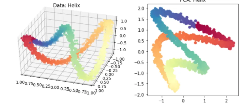
So the components are uncorrelated and their variance is the corresponding eigenvalue. Even though PCA is a linear method, it is widely used. However, when applying PCA for dimensionality reduction we encounter some limitations. Figure 2.1.1 contains the 2-dimensional embedding computed via PCA of a 3-2-dimensional helix that we will explain with detail in further sections. Unfortunately, points that are far away in the original space are near in the projection space. Observe, for example, the orange and the greenish blue points, which appear separated in the original space and overlap in the embedding space, which is not desirable.

(26)

Figure 2.1.1: Helix dataset. Left: data in the original space. Right: embedding computed via PCA.

2.2 Similarity Graphs and Laplacians

In this section we will introduce some mathematical definitions and results that will give the foundation of the Laplacian Eigenmaps and Spectral Clustering algorithms [5, 9, 3], that often outperform traditional clustering algorithms, such as k-means or single linkage [10]. Given a set of points, D={x1, . . . , xN}, and a measure of similarity,wij, betweenxi and

xj we can construct an undirected graph G = (X, E), in which the vertices, X, are the

set of points and the set of edges, E, is weighted by wij. Weights are commonly obtained

by means of a positive definite and symmetric kernel k(x, y). Given such a graph, we can define its adjacency matrix.

Definition 1 (Adjacency matrix). The adjacency matrix of the graph G is W = (wij),

with i, j= 1, . . . , N. As G is undirected, it is required that wij =wji.

The adjacency matrix will be also called similarity matrix, as it contains the similarity between points. Note thatwij = 0 implies that xi andxj are not directly connected in the

graph. This is not the standard in graph theory, as normally the edges are weighted by the cost of traveling between nodes, which is typically a decreasing function of the similarity. Thus, generally, the weight between two nodes that are not connected should be infinite. However, Similarity Graphs contain the similarity between vertices, which should be 0 if two points are not connected in the graph, i.e. the two points are not considered to be similar.

Definition 2 (Degree of a vertex). The degree of the vertex xi is computed as

d(xi) =di = N

X

j=1

wij .

Definition 3 (Degree matrix). The degree matrix of Gis D= (dij), such that

dij =

(

di ifi=j

0 otherwise. (2.2.1)

When working with subgraphs composed by a subset of vertices,A, and the edges of the graph restricted to those vertices,EA, we will write (A, EA)⊂(X, E). The complementary

(27)

2.2. Similarity Graphs and Laplacians 9

of A will be denoted as ¯A and the number of vertices in A is written as |A|. We will say

A⊂ X is connected if every pair of vertices can be connected by a path totally contained in

EA. In addition, if there are no connections betweenAand ¯A, we will sayAis a connected

component. Thus, we will sayGis connected if it only contains one connected component.

Definition 4 (Indicator vector). The indicator vector of A⊂ X, 1A, is 1A= (f1, . . . , fN)T ,

where fi= 1 ifxi∈A and 0 otherwise.

Given a dataset, D, there are several popular constructions that can be used to trans-form the data into a graph. The most used approaches are given in [5] and they are the following.

The simplest approach is the-neighborhood graph, in which two vertices are con-nected when the distance between them is less than a given parameter. As the similarity between the connected points is in the same scale (at most ), this graph is usually con-sidered as an unweighted graph. Simply, we set wij = 1 if xi and xj are connected and 0

otherwise.

We also have thek nearest neighbor graph, in which each vertex is connected with its k nearest neighbors. This approach leads to a directed graph. Depending on the ways of making the graph undirected, we can distinguish:

• The vertices xi andxj are connected ifxi is among thek nearest neighbors ofxj or

vice versa.

• The vertices xi and xj are connected if xi is among the k nearest neighbors of xj

and vice versa. This one is known as mutualknearest neighbor graph.

The first approach creates a denser graph, in the sense that it contains more edges than the second one. In this case, in contrast to the -neighborhood graph, the similarity wij

between xi and xj is set to 1 ifxi and xj are connected and to 0 otherwise.

Finally, in thetotally connected graphall vertices of G are connected by means of a kernel that represents the notion of similarity. The Gaussian kernel is commonly used, leading to the similarity

wij =k(xi, xj) = exp −

kxi−xjk2

2σ2

! ,

where σ is a parameter that controls the width of the neighborhoods and xi, xj ∈ X.

Typically, the equation of this kernel is written as

wij = exp

−γkxi−xjk2

,

where γ = ₂1_σ2. However, in this work we will the σ-notation, since it will be more comfortable when performing the experiments. Note that any symmetric and positive definite kernel can be used instead. This is the type of graph usually built in Diffusion Maps.

(28)

2.2.1 Graph Laplacians and their Basic Properties

The main tools for Spectral Clustering are graph Laplacian matrices. There exists a whole field dedicated to the study of those matrices, called Spectral Graph theory. Given a dataset D, its associated graph G, the adjacency or similarity matrix W and the degree matrixD, the graph Laplacian can be defined in two ways depending on the normalization: the Unnormalized and the Normalized graph Laplacian. For this section, it may be useful to recall the Spectral Theorem.

Theorem 1. (Spectral theorem) LetA be a symmetric matrix of dimensionN×N. Then, it can be diagonalized with an orthonormal basis, i.e., A=UΛUT, where

• Λ is a diagonal matrix with real entries, and

• the columns of U form an orthonormal basis of RN.

In the following, we do not necessarily assume that the eigenvectors are normalized so the vector v and a×v, a ∈ _R, are considered to be the same eigenvector. Eigenvalues will always be ordered from lowest to highest, respecting multiplicities. By the first k

eigenvectors we refer to the eigenvectors corresponding to thek smallest eigenvalues. Definition 5 (Unnormalized graph Laplacian). The Unnormalized graph Laplacian of a graph is defined as

L=D−W . (2.2.2)

Note that W = (wij) is a similarity matrix, so we have wij ≥ 0 for i, j = 1, . . . , N.

Some important facts of the Unnormalized graph Laplacian are summarized in the following theorem, whose proof can be found in [5].

Theorem 2. L satisfies the following properties:

1. ∀f ∈_RN_{, f}0_Lf ₌ 1 2

PN

i=1,j=1wij(fi−fj)2.

2. L is symmetric and positive semidefinite.

3. The smallest eigenvalue of L is 0. The corresponding eigenvector is the constant vector 1∈_RN_{. The normalized eigenvector would be} _√1

N ∈R N_.

4. Lhas N non-negative real eigenvalues0 =λ1 ≤λ2 ≤ · · · ≤λN and real eigenvectors.

There is another matrix which is called Normalized graph Laplacian in the literature and it is widely used when doing Spectral Clustering.

Definition 6 (Normalized graph Laplacian). We call the Normalized graph Laplacian of a similarity graph G to the matrix

Lrw =D−1L=I−D−1W .

The reason to writeLrw is that this Laplacian is related to the probability matrix of a

(29)

2.2. Similarity Graphs and Laplacians 11

Normalized graph Laplacian is closely related to the Unnormalized version. In fact, it is easy to check that λis an eigenvalue of Lrw with eigenvector v if and only if λsolves the

generalized eigenproblem

Lv=λDv . (2.2.3)

That is to say, likeL,Lrw is positive definite and hasN non-negative eigenvalues 0 =λ1 ≤

λ2 ≤ · · · ≤λN and real left eigenvectors v1, . . . , vN. The main result for the Normalized

graph Laplacian is related to the number of connected components in the graph, as detailed in Theorem 3. The proof can be found in [5].

Theorem 3. Let G = (X, E) be an undirected graph with non-negative weights. Let

A1, . . . , Ak be its connected components. Then, the multiplicity of the eigenvalue 0 in Lrw

is k. The corresponding eigenvectors are {1_A₁, . . . ,1Ak}.

2.2.2 Spectral Dimensionality Reduction and Laplacian Eigenmaps

The Laplacian Eigenmaps (LE) method is a very successful procedure for dimensionality reduction [2] while preserving local properties under certain conditions, as we will see below. In the following we will suppose a fully connected graph. Given a datasetD={xi}i=1,...,N

and a similarity measure between points,wij =k(xi, xj), the algorithm works as follows:

1. Build the undirected similarity graph G = (X =D, E) and compute the similarity matrix W following any of the approaches shown in Section 2.2.

2. Solve the problem Lv = λDv, where L and D are defined in Equations (2.2.2) and (2.2.1) respectively.

3. Compute the embedding:

Ψ :xi∈ D →(v2(xi), . . . , vd(xi)),

where vk(xi) denotes the i-th component of the k-th generalized eigenvector from

Equation (2.2.3). Note that just v1(x) is constant as we are supposing a fully con-nected graph.

The justification of this algorithm can be found in [2]. If we denote the embedding matrix by Y ∈_RN×d_{, a reasonable objective function would be to penalize points that are}

close in the original space (and hence the edge between them has a large weight) but are mapped far apart in the embedding space. Therefore, a plausible objective function is

X

i,j

kyi−yjk2wij ,

where yk denotes the embedding of the point xk, that is to say, thek-th row of Y. It can

be shown that

X

i,j

kyi−yjk2wij = trace(YTLY).

Hence, we get the following optimization problem: argmin

YT_DY₌_I

(30)

where I denotes the identity matrix. We constrained one degree of freedom in order to avoid an arbitrary solution. Since L is positive definite (see Theorem 2), this optimiza-tion problem is solved by the eigenvectors corresponding to the first d eigenvalues of the generalized problem

Lv=λDv , (2.2.4)

which will be denoted as vi,i= 1, . . . , d. That is to say, the solution is the matrix

Y = [v1, . . . , vd],

wherevj,j= 1, . . . , d, denotes thej-th solution of the Equation (2.2.4). Thus, the columns

of Y are the firstdleft eigenvectors of Lrw.

As we will see in the next section, Laplacian Eigenmaps, which are a particular case of Diffusion Maps, handle only manifolds from which the data is sampled uniformly, something that rarely happens in real Machine Learning tasks. Diffusion Maps address this problem.

2.3 Diffusion Maps

Diffusion Maps [6] are another technique for finding meaningful geometric descriptions for datasets even when the observed samples are non-uniformly distributed. Similarity graphs seen in Section 2.2 give us a powerful tool to depict the notion of geometry. In this algorithm, Coifman and Lafon provide a new motivation for Normalized graph Laplacians by relating them to Diffusion Distances.

In the original work the algorithm is motivated with continuous data, so we work in a probability space (X,A, µ) where a symmetric kernel that verifiesk(x, y)≥0 presents the notion of local structure (similarity). The degree of a vertex x∈ X is the integral

d(x) =

Z

X

k(x, y)dµ(y).

So, we define the transition probability between vertices as

p(x, y) = k(x, y)

d(x) .

Even though the kernelp(x, y) is not symmetric, it inherits the positive-preserving property of k(x, y). That is,p(x, y)≥0. In addition, we have gained the conservation property

Z

X

p(x, y)dµ(y) = 1.

This means that p can be viewed as the transition kernel of a Markov chain on X. The diffusion operator associated to p(x, y) is defined as

P f(x) =

Z

X

p(x, y)f(y)dµ(y).

We sayψ(x) is an eigenfunction, with associated eigenvalueλ, of the operatorP if it verifies

(31)

2.3. Diffusion Maps 13

In practice, we always work with finite samples. The diffusion operator is then a matrix

Pij = p(xi, xj) and p(xi, xj) is now the transition probability in a random walk defined

over the initial dataset X = {x1, . . . , xN}. In the same way, instead of working with

eigenfunctions we work with eigenvectors. The transition matrix P is related toLrw from

Definition 6 as

Lrw =I −D−1W =I −P ,

where W is the similarity matrix from Definition 1. That is, Wij =k(xi, xj), xi, xj ∈ X.

From this we can conclude that if λis an eigenvalue with right eigenvectorv ofLrw, then

1−λ is an eigenvalue with right eigenvector v of P. As a consequence of Theorem 3 we can deduce that the multiplicity of the eigenvalue λ= 1 in P is the number of connected components. In addition, if we suppose a connected graph, as P defines the transition matrix of a random walk, we can assert that P has a discrete sequence of eigenvalues

1 =λ0 > λ1≥λ2 ≥. . .≥0,

and, in addition, P ψl =λlψl, where ψl denotes the l-th eigenvector of P, which are real

eigenvectors. As already mentioned, the eigenvector associated to λ0 = 1 is constant, collapsing all the elements of each component around 1 and, therefore, not providing any information. In [6] the authors gave a measure, known as Diffusion Distance, that estab-lishes how two points are connected in a graph.

Definition 7 (Diffusion Distance). A family of Diffusion Distances {Dt}t∈_N in time t is defined as: D2_t(x, y) =kpt(x,·)−pt(y,·)k2L2₍_X_,dµ₎ = Z X (pt(x, u)−pt(y, u))2dµ(u),

where pt(x, y) denotes the probability of traveling from x toy in time t.

Note that if we have Dt(x, y) ' 0 then we also have pt(x, u) ' pt(y, u) for u ∈ X.

This means that it should be also posible to travel from x toy in timet. In practice, the integrals are intractable. Given a datasetD, the discrete version of the Diffusion Distance forx, y∈ D is

D2_t(x, y) =kpt(x, z)−pt(y, z)k2d

=X

z∈D

(pt(x, z)−pt(y, z))2d(z),

wherept(x, y) is now the probability of traveling fromx toy intsteps. The definition

is intuitive: two points are closer the more short paths (with large weights) connect them.

Dt(x, y) involves all paths of length t. Hence, it is a robust measure. In addition, this

measure can be expressed in terms of the eigenvalues and eigenvectors of P, as proved in [6].

Theorem 4. We have

D2_t(x, y) =X

l≥1

λ2_lt(ψl(x)−ψl(y))2 ,

where ψl(x) denotes the value of the l-th eigenvector of P. The case l = 0 is omitted

(32)

We have seen that the eigenvalues of P are a decreasing sequence, so the diffusion distance can be approximated up to a certain precision s(δ, t), where δ is the relative accuracy, by truncating the summation,

D_t2(x, y)'

s(δ,t)

X

l=1

λ2_lt(ψl(x)−ψl(y))2.

Choosing δ is not trivial. In [6] the authors propose the following

s(δ, t) = max{l∈_N:|λl|t> δ|λ1|t}. (2.3.1) We will identify s(δ, t) with the dimension of the embedding, which we have denoted byd. In this way, we can formally define the concept of Diffusion Map.

Definition 8 (Diffusion Map). A Diffusion Map is a function Ψt(x) :X →Rd such that

Ψt(x) =      λt₁ψ1(x) λt₂ψ2(x) .. . λt_dψd(x)      .

Theorem 5. The diffusion map Ψt : X → Y embeds the data into the Euclidean space

Y =Rd in which the Euclidean distance is approximately the diffusion distance Dt in the

original space.

Proof. The Euclidean distance between two points, y1 = Ψt(x1) and y2 = Ψt(x2), in the embedding space is kΨt(x1)−Ψt(x2)k2= d X l=1 λt_lψl(x1)−λtlψl(x2) 2 = d X l=1 λ2_lt(ψl(x1)−ψl(x2))2 'D_t2(x1, x2).

To sum up, the Diffusion Map is an embedding that projects the original data in a Euclidean space in which the Euclidean distance approximates the diffusion distance.

In this work we will try to extend the embedding given by Diffusion Maps to examples that were not in the initial dataset. The transition matrix P =D−1W is not symmetric, but when diagonalizing or giving an extension of the embedding for new patterns, it is convenient to define a symmetric kernel, whose eigenvectors compose an orthonormal basis of Rd. Therefore, it is common to define a symmetric operator as

a(xi, xj) = k(xi, xj) p d(xi) p d(xj) , (2.3.2)

and, consequently, the matrix Aij = a(xi, xj), which can be expressed in terms of the

(33)

2.3. Diffusion Maps 15

not distinguishing between right and left eigenvectors anymore (they are the same but transposed). The eigenvalues and eigenvectors of A, which will be denoted as λl and φl

respectively, are directly related to those of P (λl,ψl). We have

Aφl =λlφl. (2.3.3)

Multiplying both sides by D−1/2, we obtain

P D−1/2φl=λlD−1/2φl.

So the eigendecomposition of P can be recovered by choosing, associated with the eigen-value λl, the right eigenvector

ψl=D−1/2φl.

2.3.1 Anisotropic Diffusion

The density of the sample is not, in general, related to the geometry of the manifold. When the sampling on the manifold is not uniform, the diffusion maps may not recover the original geometry. We are interested in recovering the structure of the manifold regardless of the density of the sample, which suggests the following question: What is the influence of the density of the points and the geometry of the possible manifold underlying the data in the eigenvectors and the diffusion spectrum?

The family of Anisotropic Diffusions [6] introduces a new parameter, α, that can be tuned to specify the influence of the density of the sample points. The following is an outline of how the Anisotropic Diffusion works, emphasizing the similarities with the Diffusion Maps introduced in the previous section. Let q(x) be the density of the points on the manifold.

1. Fix σ∈_Rand a kernel kσ = exp

_−k_x₋_y_k2 2σ2 . 2. Define qσ(x) = Z X kσ(x, y)q(y)dy ,

which is an approximation of the true densityq(x), and the kernel

k(_σα)(x, y) = kσ(x, y)

qα

σ(x)qασ(y)

.

Setting α= 0 we obtain kσ(α)=kσ.

3. Define the degree in terms ofkσ(α)(x, y) as

d(_σα)(x) =

Z

X

k_σ(α)(x, y)q(y)dy ,

and define the anisotropic diffusion as

pσ,α(x, y) =

k(σα)(x, y)

d(σα)(x)

(34)

4. Apply Diffusion Maps as usual. The diffusion matrix is then (Pσ,α)ij =pσ,α(xi, xj), i, j= 1, . . . , N .

For a finite sample, the integrals are approximated by sums in the following way

q_σ(xi) = N X j=1 kσ(xi, xj), d(_σα)(xi) = N X j=1 k(σα)(xi, xj) qα_σ(xi)qασ(xj) , p_σ,α(xi, xj) = kσ(α)(xi, xj) d(_σα)(xi) .

In order to understand the impact of the new parameter α in the algorithm we may introduce the Laplace-Beltrami operator of the manifold [11]. This operator is a general-ization of the Laplace operator but applied over functions and it is related to the geometry of the manifold. We assume that the data, X, is the entire manifold. If we define the operator

Lσ,α=

I−(Pσ,α)

σ ,

then, it is proved in [11] that for any function f, it is verified

lim σ→0Lσ,αf = ∆(f q1−α) q1−α − ∆(q1−α) q1−α f , (2.3.4)

where ∆(·) denotes the Laplace-Beltrami operator. Some values of interest of α are dis-cussed in [11]:

• When α = 0 the diffusion is reduced to the classical problem with the normalized Laplacian Lrw. From the previous equation we obtain

lim σ→0Lσ,αf = ∆(f q) q − ∆(q) q f .

That is to say, the density influence is very strong in this case. Assuming an uniform distribution in the manifold, i.e., that the points are equally distributed among the manifold, then the density is a constant. Thus, we can write q =C, where C is a real number. Hence, we have ∆(q) = 0 and ∆(f q) =q∆(f). Thus we can simplify the expression to obtain

lim

σ→0Lσ,αf = ∆(f).

As we said before, assuming a constant density, the Laplace-Beltrami operator can be approximated by the graph Laplacian.

• When α = 1, if the points are actually in a submanifold of Rd, we get from Equa-tion (2.3.4)

lim

σ→0Lσ,αf = ∆(f),

so the geometry of the manifold is perfectly retrieved (in the limit). Thus, an ap-proximation of the Laplace-Beltrami operator is always obtained independently of the density and the Riemmanian geometry of the dataset can be retrieved.

(35)

2.4. Clustering 17

Figure 2.3.1: Influence of α on an helix example. Up: original curve. Down: the em-bedding via the graph Laplacian (α = 0) and the embeddings via the Laplace–Beltrami approximation (α= 1). In the latter case, the curve is perfectly unrolled

To give an idea, in Figure 2.3.1 we can see the original curve and the embedding of an helix with equation

xi=cos(θi),

yi=sen(2θi),

zi=sen(3θi),

where θi ∈(0,2π); we added Gaussian white noise with standard deviation σr = 0.5. This

example has been previously used in Section 2.1, where we saw that the 2-dimensional embedding computed via PCA was not able to retrieve the geometry of the manifold. In Figure 2.3.1, we can see that, when taking the density of the sample into account, the curve is perfectly unrolled. Note that when the density is not taken into account, spikes are observed in the embedding, corresponding to changes in the helix, where there is more density of points. When we apply α= 1 this effect disappears, and the helix is embedded into a smooth 2-dimensional circumference.

2.4 Clustering

An important and recent application of Laplacian Eigenmaps and Diffusion Maps is known as Spectral Clustering. We have noted before that both algorithms try to embed the data into a space where local magnitudes are preserved. In the case of Diffusion Maps, the data

(36)

is projected into a Euclidean space where the usual notion of distance is similar to the Diffusion Distance Dt, which is a robust measure that takes into account probabilities of

transition between points in the manifold. Recall that the quantity Dt(x, y) involves all

paths of lengthtthat connectxtoyand vice versa. As a consequence, this number is very robust to noise perturbation.

This section will also provide a practical example in which algorithms based in the euclidean distance, such ask-means in the original space, are not able to cluster the points perfectly. However, we will see that applying k-means in the embedding space for this particular dataset provides a perfect separation between classes.

2.4.1 Classic Algorithm: k-means

K-means [8] tries to find groups or clusters in the data. Firstly,K centroids are initialized,

{µ1, . . . , µK}, and each pattern is then assigned to its closest centroid. The error is defined

as J = N X n=1 K X k=1 rnkkxn−µkk2 , (2.4.1)

where rnk is 1 if the point xn is associated with the k-th centroid. The optimization is

done in two steps:

• First, rnk is updated as

rnk =

(

1 ifk= argmin_jkxn−µjk2

0 otherwise.

• Then we update the cetroidsµk by minimizing Equation (2.4.1) withrnk fixed.

Deriving (2.4.1) with respect toµk and equaling to zero, we obtain,

2

N

X

n=1

rnk(xn−µk) = 0.

Therefore, solving the equation, we finally obtain

µk= PN n=1rnkxn PN n=1rnk .

That is to say, the optimal centroid of the cluster k is the average of the points in the cluster. These steps are repeated until the centroids stop being updated or a maximum number of iterations is reached. Note that this algorithm is sensible to the notion of distance. The Euclidean distance may not be the best selection, specially if we are working with data that lies in a manifold, which is the case studied in this work.

2.4.2 Spectral Clustering

To conclude this section, let us quickly sketch the application of Diffusion Maps to Spectral Clustering algorithms. Typically in the literature [5], Spectral Clustering algorithms are

(37)

2.4. Clustering 19

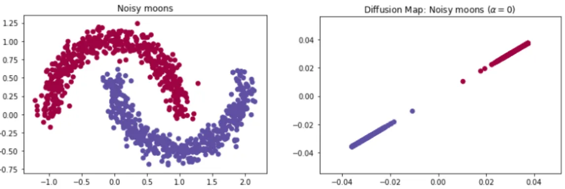
Figure 2.4.1: Spectral Clustering in the noisy moons dataset. Left: data in the original space. Right: The embedding computed via Diffusion Maps, with kernel scale σ = 0.1234 and α= 0.

focused in the embedding computed via Laplacian Eigenmaps. However, note that Lapla-cian Eigenmaps is a particular case of Diffusion Maps, in which the anisotropic parameter

α is set to 0 and the number of steps ist= 0. Given a dataset, the steps are the following:

1. Construct the similarity graph.

2. Compute the embedding, Y ⊂_Rd_{, via Diffusion Maps or Laplacian Eigenmaps.}

3. Cluster points yi ∈Y withk-means using the Euclidean distance.

The main advantage of applyingk-means in the embedding space instead of the original space is that, if the diffusion metric is right in the manifold, we will obtain better results. Close points in the manifold will also be close in the embedding space.

An illustration of the advantages of doing clustering with k-means in the embedding space is shown in Figure 2.4.1. While it is not possible to separate in two groups the image on the left with k-means (see Section 2.4.1), the Diffusion Map embedding provides a perfect separation for both targets. The noisy moons problem is linearly separable in the embedding space.

(38)

(39)

Chapter 3

Out-Of-Sample Extension

In the previous chapter we described some very foundational concepts covering the basic theory and tools that are needed in order to understand more advanced topics regarding manifold learning and dimensionality reduction when using Diffusion Maps. In this section, we will show different ways to extend the embedding given by Diffusion Maps to new patterns without re-doing the eigenanalysis over an extended similarity matrix, which is computationally expensive (O(N3)). From now on, the patterns to which we want to extend the embedding will be referred as OOS (out-of-sample). This chapter is divided into the next sections that will cover the following topics:

1. In Section 3.1 we introduce different ways to extend the embedding, depending on the target of the approximation. We will also introduce two ways to measure the low-rank approximation quality in order to compare the different approaches to OOS extensions.

2. In Section 3.2 we will explain how the Nystr¨om method can be used to define the projections of OOS patterns.

3. In Section 3.3 we will introduce a recent development that aims to merge deep learn-ing concepts with the extension of the embeddlearn-ing. In particular, a neural network will be trained to learn the encoding and decoding map.

3.1 Low-Rank Approximation

Predicting the embedding given by Diffusion Maps for an OOS example can be done following different options. The general set up, given a sample with N patterns, is as follows:

1. Select a subset of size NL of the entire sample, i.e. a subset of landmarks patterns,

and calculate the corresponding diffusion matrix, P(L), and its symmetric version,

A(L). These patterns will compose the landmark subsetL={x1, . . . , xNL}.

2. Define an extension of the resulting encoding map to be applied to the remaining

N0 =N −NL patterns, which are seen as OOS examples.

(40)

22 Chapter 3. Out-Of-Sample Extension

Landmark selection is an important problem for which several solutions have been pro-posed [12, 13]. This work is focused only on the encoding and decoding extensions, so no analysis on how to choose the subset of landmarks will be carried out. Suppose we want to give the diffusion coordinates of a new pointx. We could take two different approaches.

The first one is to learn an eigenvector extension for the OOS patterns, either from the diffusion matrix P(L)_{, or from the symmetric operator} _A(L) _{defined in Section 2.3. Once} we have the eigenvector extension, we can reconstruct the embedding for an OOS pattern

ˆ

Ψt(x), where t denotes, as usual, the number of steps. When extending the eigenvectors

of P(L) _{to a point} _x_{, we will write ˆ}_ψ

i(x), i = 1, . . . , d, where d denotes the embedding

dimension. This is the approach followed in [14]. The extension of the Diffusion Map embedding, following the scheme of Definition 8, would be

ˆ Ψt(x) i =λ t iψˆi(x),

whereλi is thei-th eigenvalue ofP(L). It is also possible to learn the eigenvector extension

at a point x for the symmetric matrix A(L). It may be useful to recall that A(L) and

P(L) have the same eigenvalues (See Section 2.3, Equation (2.3.3)). In this case, the eigenvector extension is denoted by ˆφi(x),i= 1, . . . , d. The extension to OOS patterns of

the embedding would be

ˆ Ψt(x) i = λt_i p d(x) ˆ φi(x),

whered(x) is the degree of the OOS examplex. The degree of an OOS pattern is computed by means of the kernel k(x, y), from Equation (2.3.2), and the subset of landmarks as

d(x) = X

xk∈L

k(xk, x). (3.1.1)

Another approach would be to learn directly a projection extension of the Diffusion Map, ˆΨ(x) ∈ _Rd_{, which is the approach used in [1]. The eigenvector extension for the}

matrix P(L) can be recovered as ˆ ψi(x) = ˆ Ψt(x)Λ−t i ,

where Λ is a diagonal matrix with the first deigenvalues of P(L) or A(L) in the diagonal, which are the same for both matrices. In the case ofA(L), the eigenvector extension would be ˆ φi(x) = p d(x)Ψˆt(x)Λ−t i ,

whered(x) is calculated as in Equation (3.1.1). Identifying terms in the last two equations, we can relate the extensions of the eigenvectors of P(L) and A(L) as

ˆ

φi =

p

d(x) ˆψi. (3.1.2)

When measuring the quality of the embedding to OOS patterns, there are several paths that can be followed. The first one is a straightforward approach, in which we calculate the Frobenius norm of the difference of the original matrices A and P, computed from the complete sample, and the one reconstructed using the landmark subset, so the best approach would be the one minimizing this quantity. This option is developed in Section 3.1.1. The second option, explained in Section 3.1.2, would be to directly measure the error between the original embedding and the predicted one. The problem with this method is that, when changing the data to compute de Diffusion Map, the embedding can change up to a rotation, which we have to compute.

(41)

3.1. Low-Rank Approximation 23

3.1.1 Reconstructing the Kernel Matrix

This section provides an explanation on how to measure the low-rank approximation quality of the embedding by reconstructing the matrixA. Recall that the matrixAis built using a measure of similarity between points, k(xi, xj), which is a symmetric and positive definite

kernel, as Aij =a(xi, xj) = k(xi, xj) p d(xi) p d(xj) ,

whered(xi) andd(xj) are the degrees of the patterns, as shown in Equation (2.3.2). In

Sec-tion 2.3 it was shown that the matrixAhas a discrete sequence of eigenvaluesλ0, . . . , λN−1, and eigenvectors, ψ0, . . . , ψN−1, so we can write A=UΛUT, where Λii=λi is a diagonal

matrix and U contains the eigenvectors ofA in columns, which compose an orthonormal basis. Given a landmark subsetL,Acan be decomposed as follows

A= A(L) BT B C (3.1.3) where Bpq =a(xp, xq) contains the kernel values computed for the landmark patterns and

the testing subset; and A(L) _{is the matrix calculated for the landmark subset. That is to} say, given a pair xi, xj ∈L,

(A(L))ij =a(xi, xj).

Since A(L) is also symmetric and positive definite, it has an eigenvalue decomposition. Following the notation, we will write A(L)=U(L)Λ(L) U(L)T, obtaining

A= U(L)Λ(L) U(L) T BT B C ! .

Let ˆU be the matrix with a possible OOS extension of the eigenvectors for the test set, which is composed of OOS patterns. Then, we can write an approximation for Aas

ˆ A= U(L) ˆ U Λ(L) U(L)T _ˆ UT = U (L)_ΛL _U(L)T U(L)Λ(L)UˆT ˆ UΛ(L) _U(L)T _ˆ UΛ(L)_UˆT ! .

The error will be measured with the Frobenius norm of the difference as

ERR= A−Aˆ F , (3.1.4) where kXk_F =trace(XTX),

for any matrix X. Depending on the method used to predict the embedding for an OOS pattern, this error is simplified. This fact will be developed in further sections.

3.1.2 Mean Squared Error of the Encoding

This section provides an explanation on how to measure the low-rank approximation quality of the embedding in terms of the mean squared error between the OOS extension and

(42)

the true embedding. That is the embedding computed via Diffusion Maps when using the complete sample, i.e. the OOS examples and the subset of landmarks. The process is explained in [11]. It is necessary to calculate a rotation matrix due to the possible transformations that suffers the embedding when training with different data points. Given the original embedding for the N examples, Ψ∈_RN×d_{, and the approximation ˆ}_Ψ_∈

RN×d for the OOS examples, the procedure is as follows:

• Define Sij =PkΨi(xk) ˆΨj(xk), withxk in the landmark subset andi, j= 1, . . . , d.

• Compute the singular value decomposition of S,S =UΛVT.

• Compute the rotation between Ψ and ˆΨ as the matrix R=V UT.

• Define SEq= Ψ(xq)−RΨ(ˆ xq) 2

, wherexq is in the test set.

• Finally, theM SE for the test set would be the average of theSEq,q=NL, . . . , N.

This work is focused on measuring the quality of the OOS extensions by means of the reconstruction error of the kernel matrix. This other approach may be explored in future work.

3.2 Nystr¨

om’s Encoding

This section is divided in two parts. The first part, Section 3.2.1, will explain the Nystr¨om’s approach to approximate a matrix built for an arbitrary symmetric and positive definite kernel, k(x, y). In the second part, we will adapt this method to give an OOS extension for Diffusion Maps.

3.2.1 Nystr¨om’s Low-Rank Approximation

The Nystr¨om encoding [4, 7] is useful when trying to approximate the kernel matrix,

K, from the one calculated from a landmark sample L = {x1, . . . , xNL}, by means of a symmetric and positive definite kernel

k(x, y) =X

i≥1

λiφi(x)φi(y),

where λi ≥0. The matrix K(L) associated to k(x, y) for the given landmark sample L is

K_ij(L)=k(xi, xj), with xi, xj ∈L.

Hence,K(L) is symmetric and positive definite and, by the spectral theorem, we can write

K(L)V(L)=V(L)Λ(L),

where Λ(L) is a diagonal matrix with diagonal λ(₁L) ≥λ₂(L) ≥ . . . ≥λ_N(L) ≥ 0 and V(L) is the matrix with the eigenvectors in columns. That is to say,

NL

X

k=1

(43)

3.2. Nystr¨om’s Encoding 25 or, equivalently, V_ji(L)= 1 λ(_iL) NL X k=1 k(xj, xk)V (L) ki . (3.2.1)

We can identify each row of V(L) with the image of each example inL. So, for anyxj ∈L,

we define the function

Vi(xj) =V_ji(L), 1≤i≤d .

That is to say, Vi(xj) denotes the i-th component of thej-th row ofV(L). Equation (3.2.1)

suggests to define the Nystr¨om extension to a newx /∈Lthrough the kernel valuesk(x, xk),

xk∈L, as ˆ Vi(x) = 1 λ(_iL) NL X k=1 k(x, xk)V_ki(L).

3.2.2 Nystr¨om’s Method and Diffusion Maps

As shown above, the Nystr¨om’s encoding can be applied as long as the kernel is symmetric and definite positive. Therefore, in the context of Diffusion Maps, it can be applied to the kernel a(x, y) to extend the eigenvectors ofA to OOS examplesx as

ˆ φi(x)' 1 λi NL X k=1 a(x, xk)φi(xk),

where φi(xk) denotes the k-th element of the i-th eigenvector of A. Note that we write

φi(·) to refer both to an eigenfuction of the operator associated to the kernela(x, y) and to

an eigenvector of A. This is because the theory of Diffusion Maps is developed in the con-tinuous case, but when working with finite datasets, the eigenfunctions are approximated by eigenvectors.

In addition, it is easy to check that the Nystr¨om’s method can be also directly applied toP, obtaining the equation

ˆ ψi(x)' 1 λi NL X k=1 p(x, xk)ψi(xk).

To prove it, we have

ˆ ψi(x) = ˆ φi(x) p d(x) = 1 λi p d(x) NL X k=1 a(x, xk)φi(xk) = 1 λi NL X k=1 k(x, xk) d(x)pd(xk) φi(xk) = 1 λi NL X k=1 p(x, xk) φi(xk) p d(xk) = 1 λi NL X k=1 p(x, xk)ψi(xk),

(44)

where we have used the relation between the extensions of the eigenvectors of Equa-tion (3.1.2), ˆφi =

p

d(x) ˆψi.

Equivalently, the OOS extension for the matrix containing the eigenvectors of A can be written as

ˆ

Uqi = ˆφi(xq) = (BU(L)(Λ(L))−1)qi ,

where ˆU denotes the approximation for U,q =NL, . . . , N are the indices of the OOS set

and B,U(L) and Λ(L) are the same as in Equation (3.1.3). The low-rank approximation ˆA

is then ˆ A= U(L) ˆ U Λ(L) U(L)T _ˆ UT = A (L) _U(L)_Λ(L)_(Λ(L)₎−1₍_U(L)₎T_BT BU(L)_(Λ(L)₎−1_Λ(L) _U(L)T BU(L)_(Λ(L)₎−1_Λ(L)_(Λ(L)₎−1₍_U(L)₎T_BT ! = A(L) BT B B(A(L))−1BT .

Thus the reconstruction error when using the Nystr¨om approximation [12] to extend the eigenvector of A would be, substituting in Equation (3.1.4),

ERRnys= C−B(A (L)₎−1_BT 2 F , (3.2.2) where Bkq=a(xk, xq) = k(xk, xq) p d(xk) p d(xq) , with xk∈L, xq∈/L, and Cpr =a(xp, xr) = k(xp, xr) p d(xp) p d(xr) , withxp, xr ∈/L .

3.3 Diffusion Nets

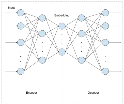
The aim of Diffusion Nets [1] is to employ deep learning from a manifold learning perspec-tive. The authors address three problems: OOS embeddings of new points, a pre-image solution that can include regularization, and outlier detection on test data. The proposal is to train two neural networks, which will be referred as encoder and decoder, and combine them in an autoencoder. Of these three we will study the encoder solution as an OOS extension method.

3.3.1 Artificial Neural Networks

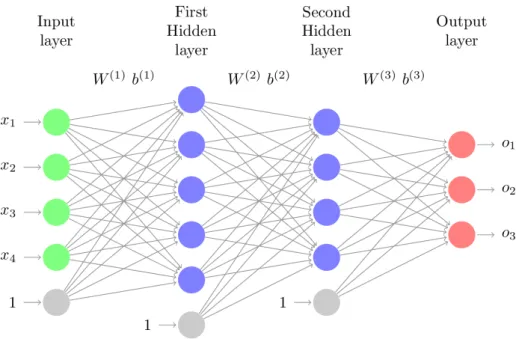
Artificial Neural Networks (ANNs) are networks composed of connected units, which are called neurons. A particular example is the Multilayer Perceptron (MLP), a network with fully connected layers. An example of a MLP can be seen in Figure 3.3.1. The output of each layer is computed as

o(l+1) =h(W(l)o(l)+b(l)),

whereh(·) is a non-linear function called activation,W(l)are the weights that connect the neurons in the layer lwith those in the layerl+ 1, o(l) is the output of the previous layer

(45)

3.3. Diffusion Nets 27

Figure 3.3.1: Standard Multilayer Perceptron with two hidden layers.

andb(l)is a bias term. The set of weights is defined as Θ ={W(l), b(l)}. We denote byLthe number of layers in the network and by sl the number of neurons in the layerl, 1≤l≤ L.

The experiments carried out in [1] are done using the sigmoidal as the activation for the hidden layers. This is

h(z) =σ(z) = 1 1 +e−z .

Other choices may include h(z) = tanh(z) or the rectified linear units,

h(z) = ReLU(z) = max{0, z}.

Particularly, these kind of networks can be used for regression. Following the standard for regression, the activation functions for the output layer are the identity. The training set will be composed of N observations

D={(x1, y1), . . . ,(xN, yN)},

where xi ∈Rd and yi∈Rm,i= 1, . . . , N. The MLP is, thus, a function

o:Rm→Rd

x7→o(x,Θ),

wheremdenotes the input dimension,dis the output dimension and Θ is the set of weights of the neural network. When we refer to the complete output matrix, which contains the image by the MLP of all the patterns in our dataset, we will write O. These parameters are chosen to minimize a loss function. For this purpose, gradient descent based methods are used. The gradient is computed with the back propagation algorithm. For regression problems the standard regularized loss function is

JREG(Θ) = 1 2N N X i=1 ko(xi,Θ)−yik2+ µ 2 L−1 X l=1 W (l) 2 , (3.3.1)

(46)

Figure 3.3.2: Autoencoder. Left: encoder with one hidden layer. Right: decoder with one hidden layer.

where µ is a parameter to control the importance of the regularization term. This term aims to avoid overfitting.

3.3.2 OOS Example Extension: the Encoder

When using a neural network to predict the embedding for OOS examples, we will assume the data lies on a smooth, compact, d-dimensional Riemannian manifold. The Diffusion Map for the training set embeds the landmark subsetL={x1, . . . , xNL}into the Euclidean spaceRd. The diffusion embedding is denoted by Ψ∈RN×d, which is a matrix whose rows correspond to the embeddings computed for the training points.

Given new test points,X0 ={xq}q=NL,...,N, the aim is to calculate an approximation as close as possible to the true embedding. For each test pointxq ∈ X0, we will write ˆΨ(xq) to

denote the embedding approximation. It is also desirable that the approximation preserves the original properties of the embedding. With this purpose, the encoder is designed as an MLP, minimizing the L2 loss between the diffusion embedding Ψ and the output of the net, which is denoted by Oe∈ _RN×d_{. Since the coordinates of the Diffusion Map are}

eigenvectors of the random walk matrix on the data,P, thej-th column ofOeshould fulfill

P O_je'λjOej ,1≤j≤d . (3.3.2)

where, as usual, λj denotes the j-th eigenvalue of P.

The architecture of the encoder is shown in the left part of Figure 3.3.2 and the algo-rithm to train the encoder is shown in Algoalgo-rithm 1. The set up is: define a MLP with L

(47)

3.3. Diffusion Nets 29

hidden layers whose output layer is a regression layer (i.e. the identity is its activation) and minimize the loss function defined in (3.3.1). However, the authors of [1] proposed a modified loss function,

Je(Θ) =JREG(Θ) +JEV(Θ), (3.3.3) where JREG is the standard regularized loss for regression of Equation (3.3.1) and

JEV(Θ) = η 2NL d X j=1 (P−λ_jI_N_L×NL)O e j 2 , (3.3.4)

where η is an optimization cost parameter and INL×NL denotes the identity matrix of dimension NL. They also provide a calculation for the gradient of this loss function with

respect to the output layer, which is

∇JEV = η NL d X j=1 (O_je)T(PT −λjINL×NL)(P −λjINL×NL).

The aim of the penalization of Equation (3.3.4) is to force the output of the neural network to be eigenvectors of the Diffusion Matrix P, so the embedding still conserves its initial properties. The value ofη has to be chosen carefully because, otherwise, the output will be forced to be 0. In contrast to general constraints, this restriction needs output values of the different test points together. For this reason, using this term can lead to computational problems, as the new gradient cannot be decomposed to use online training because the loss function needs the values predicted to all the examples in order to be evaluated. In [1] it is shown that incorporating this term does not lead to extremely better solutions, so in this work we will not consider (3.3.4).

Algorithm 1:Encoder

Input: Training set X, diffusion embedding Ψ for X, number of layers L, neurons per layersl,l= 1, . . . ,L.

Output: None

1: Initialize the weights Θ of the encoder and set X as input and Ψ as target. 2: Train the network minimizing (3.3.3) with back-propagation

Once we have a prediction for the test set, there are different ways to measure the quality of the approximation. In the original work [1], they used the approach explained in Section 3.1.2, measuring the MSE made by the encoder using LOOCV (Leave One Out Cross Validation). However, this approach does not verify that the predicted embedding fulfills the property of Equation (3.3.2) and we may lose the eigenvalue structure of the embedding.

The authors not only proposed in [1] an extension of the embedding to OOS using neural networks. They also provide a theoretical bound on the error rate for approximating eigenfunctions of the Laplacian using a MLP with sigmoids activations. Suppose M ⊂_Rn

a d-dimensional manifold.

Definition 9 (Locally bi-Lipschitz metric). We say ρ : M × M → R+ is a locally

bi-Lipschitz metric with respect to the Euclidean metric if ∀∃δ such that kx−yk ≤δ then,