How To Create A Triangulation From A Point Cloud

R. Scopigno, D. Zorin, (Editors)

Spectral Surface Reconstruction from Noisy Point Clouds

University of California, Berkeley

Abstract: We introduce a noise-resistant algorithm for reconstructing a watertight surface from point cloud data. It forms a Delaunay tetrahedralization, then uses a variant of spectral graph partitioning to decide whether each tetrahedron is inside or outside the original object. The reconstructed surface triangulation is the set of triangular faces where inside and outside tetrahedra meet. Because the spectral partitioner makes local decisions based on a global view of the model, it can ignore outliers, patch holes and undersampled regions, and surmount ambiguity due to measurement errors. Our algorithm can optionally produce a manifold surface. We present empirical evidence that our implementation is substantially more robust than several closely related surface reconstruction programs.

Categories and Subject Descriptors(according to ACM CCS): I.3.5 [Computing Methodologies]: Computer Graph-ics Computational Geometry and Object Modeling

1. Introduction

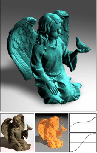
Laser range finders record the geometry of real-world three-dimensional objects in the form of point coordinates sam-pled from their surfaces, plus auxiliary information such as the laser’s position. Surface reconstruction algorithms recreate geometric models from these data, expressed in a form more useful for applications such as rendering or simulation—for example, as a surface triangulation or as splines. Laser range finders are imperfect devices that in-variably introduce at least two kinds of errors into the data they record: measurement errors (random or systematic) in the point coordinates, and outliers, which are spurious points far from the true surface. Furthermore, objects often have regions that are not accessible to scanning and so remain undersampled or unsampled. The point cloud in Figure 1 (bottom center) suffers from all the above.

When these problems are severe, data arise for which no algorithm can construct an accurate, consistent, watertight model of an object’s surface solely by examining local re-gions of a point cloud independently. A successful algorithm must take a global view.

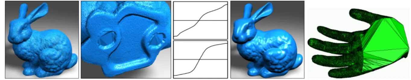
Figure 1: A watertight manifold surface triangulation re-constructed by our eigencrust algorithm; a photograph of the source object; the point cloud input to the algorithm, with 4,000 artificial random outliers; and the sorted com-ponents of the two eigenvectors used for the reconstruction. 2,008,414 input points; 12,926,063 tetrahedra; 3,605,096 output triangles; genus 14 (source object has genus 1); 437 minutes reconstruction time, including 13.5 minutes to tetra-hedralize the point cloud, and 157 minutes and 265 minutes to compute the first and second eigenvectors, respectively.

Our innovation is to introduce the techniques of spectral partitioning and normalized cuts into surface reconstruction. These techniques are used heavily for tasks such as image segmentation and parallel sparse matrix arithmetic, where partitioning decisions based on a global view of an image or a matrix can outperform local optimization algorithms. Although the global optimization step makes our algorithm slower than many competitors, it reconstructs many models that other methods cannot.

The general technique we use to produce a surface from a point cloud is well known: compute the Delaunay tetrahe-dralization of the points, then label each tetrahedroninside

oroutside. (Recent advances in Delaunay software make it possible to tetrahedralize sets of tens of millions of points.) The output is a triangulated surface, composed of every tri-angular face where aninsidetetrahedron meets anoutside

tetrahedron. This procedure guarantees that the output sur-face is watertight—it bounds a volume, and there is no route from the inside to the outside of the volume that does not pass through the surface. Watertight surfaces are important for applications such as rapid prototyping and volume mesh generation for finite element methods.

Our contribution is an algorithm for labeling the tetrahe-dra that is substantially more robust than previous methods. We call the surface it produces the eigencrust. The eigen-crust algorithm creates a graph that represents the tetrahedra. A spectral partitioner slices it into two subgraphs, aninside

subgraph and anoutsidesubgraph. Because the spectral par-titioner has a global view of the point set, it is effective at identifying the triangular faces that are most likely to lie at the interface between an object and the space around it.

2. Related work

There has been much work on reconstructing surfaces from point clouds. The idea of labeling each Delaunay tetrahe-droninsideor outside, then extracting a surface using the labels, appears in an early paper of Boissonnat [Boi84], and is also harnessed in the Tight Cocone algorithm of Dey and Goswami [DG03] and in the Powercrust algorithm of Amenta, Choi, and Kolluri [ACK01] (with cells of a power diagram replacing tetrahedra). In this paper, we compare implementations of the Tight Cocone and Powercrust algo-rithms with our eigencrust software.

A recent advance is the Robust Cocone algorithm of Dey and Goswami [DG04], a Delaunay-based reconstruction al-gorithm that is provably robust against small coordinate er-rors. Their algorithm is not robust against undersampling or outliers, and in fact is easily defeated by undersampling. We observe that a variant of our spectral algorithm could be used to help the Robust Cocone algorithm to label tetrahe-dra when the sample set is not dense enough for the Robust Cocone’s original labeling algorithm to succeed. Unfortu-nately, we did not have sufficient time to obtain a Robust Cocone implementation for comparison in this paper.

Another branch of surface reconstruction algorithms are those that define a function over space whose zero set is a surface, which can be triangulated by techniques such as marching cubes [LC87]. These algorithms vary widely in how they compute the function. Hoppe, DeRose, Duchamp, McDonald, and Stuetzle [HDD∗92] provide one of the ear-liest algorithms, which locally estimates the signed distance function induced by the “true” surface being sampled. Bit-tar, Tsingos, and Gascuel [BTG95] use the medial axis of the point set to improve the speed of zero-set methods and their ability to reconstruct topologically complex objects. Cur-less and Levoy [CL96] developed an algorithm that is par-ticularly effective for laser range data comprising billions of point samples, like the statue of David reconstructed by the Digital Michelangelo Project [LPC∗00]. A zero-set ap-proach by Carr et al. [CBC∗01] adapts the radial basis func-tion-fitting algorithm of Turk and O’Brien [TO99] to sur-face reconstruction. Ohtake, Belyaev, Alexa, Turk, and Sei-del [OBA∗03] use a partition-of-unity method with a fast hierarchical evaluation scheme to compute surfaces for data sets with over a million points.

Closely related to the zero-set approaches are the level-set algorithms of Whitaker [Whi98] and Zhao, Osher, and Fed-kiw [ZOF01]. Other important reconstruction algorithms are the mesh zippering algorithm of Turk and Levoy [TL94], Bernadini et al.’s [BMR∗99] ball-pivoting algorithm, and Kobbelt, Botsch, Schwanecke, and Seidel’s [KBSS01] meth-od for extracting surfaces from volumetric data, which in-cludes effective methods of extracting sharp corners that are often missed by marching cubes.

Different branches of algorithms have different advan-tages. The main advantages of the Delaunay algorithms are the effortlessness with which they obtain watertight surfaces; the ease with which they adapt the density of the triangles to match the density of the points (unlike marching cubes), for models whose point density varies greatly from region to region; and the theoretical apparatus that makes it pos-sible to prove the correctness of some of these reconstruc-tion algorithms on well-sampled smooth surfaces [ABK98, AB99, AK00, ACDL02]. Here, we show that spectral parti-tioning can help make these methods robust for surfaces that are noisy or not sufficiently well-sampled for the theoretical guarantees to apply.

Spectral methods for partitioning graphs were introduced by Hall [Hal70] and Fiedler [Fie73] and popularized by Pothen, Simon, and Liou [PSL90]. They are used for tasks such as image segmentation, circuit layout, document clus-tering, and sparse matrix arithmetic on parallel computers. The goal of graph partitioning is to cut a graph into two sub-graphs, each roughly half the size of the original graph, so that the total weight of the cut edges is small (each edge is assigned a numerical weight). There are many ways to for-mulate the graph partitioning problem, which differ in how they trade off the weight of the cut against the balance be-tween the two subgraphs. Most graph partitioning formula-tions are NP-hard, so practical partitioning algorithms

(in-cluding spectral methods) are heuristics that try to find an approximate solution.

One of the most effective formulations of spectral par-titioning is the normalized cuts criterion of Shi and Ma-lik [SM00], which is particularly effective at trading off sub-graph balance against cut weight. We make a simple modifi-cation to the Shi–Malik algorithm (closely related to a tech-nique of Yu and Shi [YS01]) that greatly improves our sur-face reconstruction algorithm’s speed and the quality of the surfaces it produces.

3. Spectral Surface Reconstruction

We assume the reader is familiar with the notions of De-launay triangulations and Voronoi diagrams in three dimen-sions, and with the geometric duality that maps each Delau-nay tetrahedron to a Voronoi vertex and each DelauDelau-nay face to a Voronoi edge. See Fortune [For92] for an introduction.

The eigencrust algorithm begins with a set S of sample points in space. Let S+be the set S augmented with eight bounding box vertices, the corners of a large cube that en-closes the sample points. (The width of the cube should be much greater than the diameter of S, so that no sample point lies near any side of the cube). Let T be the Delaunay tetra-hedralization of S+. Let Q be the Voronoi diagram of S+ (and the geometric dual of T ). For each tetrahedron t in the tetrahedralization T , there is a dual vertex v of the Voronoi diagram Q, and v is the center of the sphere that circum-scribes t.

The goal is to label each tetrahedron—or equivalently, each Voronoi vertex—insideoroutside. The eigencrust al-gorithm labels the Voronoi vertices in two stages. Each stage forms a graph and partitions it.

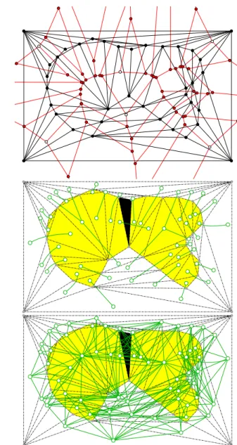
In the first stage, our algorithm labels a subset of the Voronoi vertices called the poles, following Amenta and Bern [AB99]. We form a graph G, called the pole graph, whose nodes represent the poles. See Figure 2 for a two-dimensional example. The edges of G are assigned numer-ical weights that reflect the likelihood that certain pairs of poles are on the same side of the unknown surface that we wish to reconstruct.

The graph G is represented by a pole matrix L. We par-tition the poles of G by finding the eigenvector x that corre-sponds to the smallest eigenvalue of a generalized eigensys-tem Lx=λDx, and using that eigenvector to cut the graph into two pieces, theinsideandoutsidesubgraphs. Thus we label each poleinsideoroutside.

In the second stage, we form another graph H whose nodes represent the Voronoi vertices that are not poles, and partition H to label all the Voronoi vertices (equivalently, the tetrahedra) that were not labeled in the first stage. The goal of the second stage is different from the goal of the first: the non-poles are somewhat ambiguous—most of them could arguably be eitherinsideoroutside—so the partitioner

Figure 2: Top: the Delaunay triangulation (black) and Voronoi diagram (red) of a set of points sampled from a closed curve. Red Voronoi vertices are poles; white Voronoi vertices are not. Note that three-dimensional examples have many more non-pole Voronoi vertices than two-dimensional examples. Center: the negatively weighted edges of the pole graph G (green), before the bounding box triangles are col-lapsed into a single supernode. Yellow triangles are the du-als of poles labeledinsideby the first stage of spectral par-titioning. The black triangle does not dualize to a pole; it is labeledinsideby the second partitioning stage. Bottom: the positively weighted edges of G.

tries to assign them labels that produce a relatively smooth surface with low genus.

Now all the Voronoi vertices have labels, so all the tetra-hedra of T have labels. The eigencrust is a surface

triangula-tion consisting of every triangular face of T where aninside

tetrahedron meets anoutsidetetrahedron. If the points in S are sampled densely enough from a simple closed surface, then the eigencrust approximates the surface well.

If all the tetrahedra adjoining a sample point are labeled

outside(or all areinside), the point does not appear in the reconstructed surface triangulation. In Section 4, we see that this effect provides our algorithm with effective and auto-matic outlier removal. No other effort to identify outliers is required.

Why are the Voronoi vertices labeled in two separate stages? Because the non-poles are ambiguous, they tend to “glue” the inside and outside tetrahedra together. If they are included in the first partitioning stage, the graph partitioner is much less successful at choosing the right labels, and runs more slowly too. A two-stage procedure produces notably better and faster results.

We have chosen the graphs’ edge weights (by trial and error) so the algorithm tries to emulate the provably correct Cocone algorithm of Amenta et al. [ACDL02] when there is neither noise nor outliers, and the sampling requirements of the Cocone algorithm are met. Our algorithm usually returns significantly different results only under conditions where the Cocone algorithm has no guarantee of success.

Our algorithm includes three optional steps. After the first partitioning stage, we can identify some tetrahedra that may be mislabeled due to noise, and remove their labels (so they are assigned new labels during the second stage). This step improves the resilience of our algorithm to measurement er-rors. After the second partitioning stage, we can convert the surface to a manifold (if it is not one already) by relabeling someinsidetetrahedraoutside. After the final surface recov-ery step, we can smooth the surface to make it more useful for rendering and simulation.

3.1. The Pole Graph

Imagine that we form a graph whose nodes represent the ver-tices of the Voronoi diagram Q (and their dual tetrahedra in T ), and whose edges are the edges of Q (omitting the edges that are infinite rays). Suppose we then assign appropriate weights to the edges, and partition the graph intoinsideand

outsidesubgraphs.

Unfortunately, this choice leads to poor results. The main difficulty is that the Delaunay tetrahedralization T invari-ably includes flat tetrahedra that lie along the surface we are trying to recover, as Figure 3(a) illustrates. These tetra-hedra are not eliminated by sampling a surface extremely finely; they are a natural occurrence in Delaunay tetrahe-dralizations. Many of them could be labeledinsideor out-sideequally well. They cause trouble because they can form strong links with both the tetrahedra inside an object and the tetrahedra outside an object, and thus prevent a graph parti-tioner from finding an effective cut between the inside and outside tetrahedra. v u s c (a) (b)

Figure 3: (a) No matter how finely a surface is sampled, tetrahedra can appear whose circumscribing spheres are centered on or near the surface being recovered. (b) The Voronoi cell c of a sample point s. The poles of s—the Voronoi vertices u and v—typically lie on opposite sides of the surface being recovered, especially if the cell is long and thin.

To solve this problem, Amenta and Bern [AB99] iden-tify special Voronoi vertices called poles. Poles are Voronoi vertices that are likely to lie near the medial axis of the sur-face being recovered. The Voronoi vertices whose duals are the troublesome flat tetrahedra are rarely poles, because the problem tetrahedra lie near the object surface, not near the medial axis.

Each sample point s in S can have two poles. Let c be the Voronoi cell of s in Q (i.e. the region of space composed of all points that are as close or closer to s than to any other sample point in S+). See Figure 3(b) for an example. The Voronoi cell c is a convex polyhedron whose vertices are Voronoi vertices. It is easy to compute the vertices of c, because they are the centers of the circumscribing spheres of the tetrahedra in T that have s for a vertex.

Let u be the vertex of c furthest from s; u is called a pole of s. Let v be the vertex of c furthest from s for which the angle∠usv exceeds 90◦; v is also called a pole of s. Fig-ure 3(b) illustrates the two poles of a typical sample point. The eight bounding box vertices in S+are not considered to have poles. Let V be the set of all the poles of all the samples in S.

Amenta and Bern show that in the absence of noise, the tetrahedra that are the duals of the poles are likely to extend well into the interior or exterior of the object whose surface is being recovered. The tetrahedra whose duals are not poles often lie entirely near the surface, as Figure 3(a) shows, so it is ambiguous whether they are inside or outside the object.

The eigencrust algorithm identifies the set V of all poles, then constructs a sparse pole graph G= (V,E). The set E of edges is defined as follows. For each sample s with poles u and v,(u,v)is an edge in E. For each pair of samples s, s0 such that(s,s0)is an edge of the Delaunay tetrahedralization T , let u and v be the poles of s, and let u0and v0be the poles of s0; then the edges (u,u0), (u,v0), (v,u0), and (v,v0)are all edges of E. Every pole is the dual of a tetrahedron, so tetrahedra that adjoin each other are often linked together in G, whereas tetrahedra that are not close to each other are not linked.

Cv Cu φ v u t t v u s v φ u Cv Cu (a) (b)

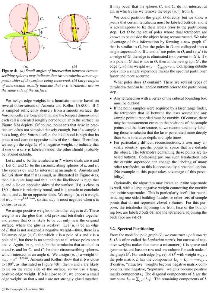
Figure 4: (a) Small angles of intersection between circum-scribing spheres may indicate that two tetrahedra are on op-posite sides of the surface being recovered. (b) Large angles of intersection usually indicate that two tetrahedra are on the same side of the surface.

We assign edge weights in a heuristic manner based on several observations of Amenta and Kolluri [AK00]. If S is sampled sufficiently densely from a smooth surface, the Voronoi cells are long and thin, and the longest dimension of each cell is oriented roughly perpendicular to the surface, as Figure 3(b) depicts. Of course, point sets that arise in prac-tice are often not sampled densely enough, but if a sample s has a long, thin Voronoi cell c, the likelihood is high that its poles u and v are on opposite sides of the surface. Therefore, we assign the edge(u,v)a negative weight, to indicate that if one of u or v is labeledinside, the other should probably be labeledoutside.

Let tuand tvbe the tetrahedra in T whose duals are u and v. Let Cuand Cvbe the circumscribing spheres of tuand tv.

The spheres Cuand Cvintersect at an angleφ. Amenta and

Kolluri show that ifφis small, as illustrated in Figure 4(a), then c is quite long and thin, and the likelihood is high that tuand tvlie on opposite sides of the surface. Ifφis close to

180◦, then c is relatively round, and it is unsafe to conclude that tuand tvlie on opposite sides. We assign(u,v)a weight

of wu,v=−e4+4 cosφ, so that wu,vis most negative whenφis

closest to zero.

We assign positive weights to the other edges in E. These weights are the glue that hold proximal tetrahedra together and ensure that G is likely to be cut only near the original surface, where the glue is weakest. Let(u,v)be an edge of E that is not assigned a negative weight—thus, there is a Delaunay edge(s,s0)for which u is a pole of s and v is a pole of s0, but there is no sample point s00whose poles are u and v. Again, let tuand tvbe the tetrahedra that are dual to u and v, and let Cuand Cvbe their circumscribing spheres,

which intersect at an angleφ. We assign(u,v)a weight of wu,v=e4−4 cosφ. Amenta and Kolluri show that ifφis close

to 180◦, as illustrated in Figure 4(b), then u and v are likely to lie on the same side of the surface, so we use a large, positive edge weight. Ifφis close to 0◦, we choose a small edge weight, so that u and v are not strongly glued together.

It may occur that the spheres Cuand Cvdo not intersect at

all, in which case we remove the edge(u,v)from E. We could partition the graph G directly, but we know a priori that certain tetrahedra must be labeledoutside, and it is advantageous to fix their labels prior to the partitioning step. Let O be the set of poles whose dual tetrahedra are known to be outside the object being reconstructed. We take advantage of this information by forming a new graph G0 that is similar to G, but the poles in O are collapsed into a single supernode z. If u and u0are poles in O, and(u,u0)is an edge of G, the edge is eliminated (not present in G0). If v is a pole in G that is not in O, then in the new graph G0, the edge(z,v)has weight wz,v=∑u∈Owu,v. Collapsingoutside

poles into a single supernode makes the spectral partitioner faster and more accurate.

What poles does O contain? There are several types of tetrahedra that can be labeledoutsideprior to the partitioning step.

• Any tetrahedron with a vertex of the cubical bounding box must beoutside.

• If the point samples were acquired by a laser range finder, the tetrahedra that lie between the laser source and any sample point it recorded must beoutside. Of course, there may be measurement errors in the positions of the sample points and the laser source, so we recommend only label-ing those tetrahedra that the laser penetrated more deeply than some tolerance depth, multiple times.

• For particularly difficult reconstructions, a user may vi-sually identify specific points in space that are outside the object. The tetrahedra containing these points are la-beledoutside. Collapsing just one such tetrahedron into the outsidesupernode can change the labeling of many other tetrahedra, so this is occasionally a practical option. (No example in this paper takes advantage of this possi-bility.)

Optionally, the algorithm may create aninsidesupernode as well, with a large negative weight connecting theoutside

andinsidesupernodes. This is particularly useful for recon-structing one-sided building facades or other sets of sample points that do not represent closed volumes. For this pur-pose, the tetrahedra adjoining the front face of the bound-ing box are labeledoutside, and the tetrahedra adjoining the back face areinside.

3.2. Spectral Partitioning

From the modified pole graph G0, we construct a pole matrix L. (L is often called the Laplacian matrix, but our use of neg-ative weights makes that name a misnomer.) L is sparse and symmetric, and has one row and one column for each node of the graph G0. For each edge(vi,vj)of G0with weight wvi,vj,

the pole matrix L has the components Li j=Lji=−wvi,vj.

(Positive, “attractive” weights become negative matrix com-ponents, and negative, “repulsive” weights become positive matrix components.) The diagonal components of L are the row sums Lii=∑j6=i|Li j|. The remaining components of L

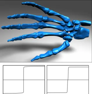
Figure 5: Watertight skeleton surface, and the sorted com-ponents of the eigenvectors computed during the two par-titioning stages. The points are densely sampled from a smooth surface, so the eigenvectors are polarized. 327,323 input points; 2,334,597 tetrahedra; 654,596 output trian-gles; genus zero; 12.3 minutes reconstruction time, includ-ing 2.8 minutes for the tetrahedralization, and 5.1 minutes and 4.2 minutes for the eigenvectors.

(the off-diagonal components not represented by an edge of G0) are zero. If G0is connected (which is always true in our application) and includes at least one edge with a negative weight, L is guaranteed to be positive definite.

The spectral analysis of a Laplacian matrix or pole ma-trix can be intuitively understood by analogy to the vibra-tional behavior of a system of masses and springs. Imagine that each node of G0represents a mass located in space, and that each edge represents a spring connecting two masses. Positive edge weights imply attractive forces, and negative edge weights imply repulsive forces. The eigensystem of L represents the transverse modes of vibration of the mass-and-spring system. The lowest-frequency modes give clues as to where the graph can be cut most effectively: theinside

masses are usually found vibrating out of phase with the out-sidemasses.

We take advantage of this observation by finding the eigenvector x associated with the smallest eigenvalueλ of the generalized eigensystem Lx=λDx, where D is a diago-nal matrix whose diagodiago-nal is identical to that of L. Because L is sparse, we compute the eigenvector x using the iterative Lanczos algorithm [Lan50, PSL90]. Each component of the eigenvector x corresponds to one column of L, and therefore to one node of G0, to one pole of Q, and to one tetrahedron of T . (The exception is the component of x that corresponds to the supernode z.)

Figure 5 shows a reconstruction of a skeletal hand and the eigenvectors computed during the two partitioning stages. The components of the eigenvectors are sorted in increasing order. When our method is applied to noise-free point sets that are densely sampled from smooth surfaces, we find that the eigenvector x is relatively polarized: most of its compo-nents are clearly negative or clearly positive, with few com-ponents near zero. However, noisy models produce more ambiguous labels—see Figures 1, 6, and 8. One of the com-ponents of x corresponds to theoutsidesupernode z. Sup-pose this component is positive; then the nodes of G0whose components are positive are labeledoutside, and the nodes whose components are negative are labeledinside. (If the component corresponding to z is negative, reverse this label-ing.)

This procedure differs from the usual formulation of malized cuts [SM00] in one critical way. The standard nor-malized cuts algorithm does not use negative weights, so its Laplacian matrix L is positive indefinite—it has one eigen-value of zero, with an associated eigenvector whose compo-nents are all 1. Therefore, the standard formulation uses the eigenvector associated with the second-smallest eigenvalue (called the Fiedler vector) to dictate the partition. Our pole graph has negative weights, our pole matrix is positive def-inite, and we use the eigenvector associated with the small-est eigenvalue to dictate the partition. Because the negative weights encode information about tetrahedra that are likely to be on opposite sides of a surface, we find that this formula-tion reconstructs better surfaces, and permits us to calculate the eigenvector much more quickly than normalized cuts in their standard form.

The Lanczos algorithm is an iterative solver which typi-cally takes about O(√n)iterations to converge, where n is the number of nodes in G0. (L is an n×n matrix.) The convergence rate also depends on the distribution of eigen-values of the generalized eigensystem, in a manner that is not simple to characterize and is not related to the condition number. The most expensive operation in a Lanczos itera-tion is matrix-vector multiplicaitera-tion, which takes O(n)time because L is sparse.

For undersampled and noisy models, the O(n√n)running time is justified. Because spectral partitioning searches for a cut that is “good” from a global point of view, it elegantly patches regions that are undersampled or not sampled at all (see Figure 6). Measurement errors may muddy up the edge weights, but a good deal of noise must accumulate globally before the reconstruction is harmed (see Section 4). There are many faster surface reconstruction algorithms, and they are often preferable for clean models. But most algorithms are fooled by undersampling, outliers, and noise, and many leave holes in the reconstructed surface or make serious er-rors in deciding how to patch holes.

Figure 6: Left: the eigencrust reconstruction of the Stanford Bunny data (raw, unsmoothed point samples with natural noise but no outliers) patches two unsampled holes in the bottom of the bunny. The eigenvectors are less polarized than the eigenvectors in Figure 5, reflecting the labeling ambiguities due to measurement errors. Also illustrated is the bunny after Laplacian smoothing, described in Section 3.6. 362,272 input points; 2,283,480 tetrahedra; 679,360 output triangles; genus zero; 19.1 minutes reconstruction time, of which 17.5 minutes is spent computing the eigenvectors. Right: the eigencrust patches a large unsampled region of a model of a hand.

3.3. Correcting Questionable Poles

An optional step, strongly recommended for noisy models, removes labels whose accuracy is questionable, so that some poles will be relabeled during the second step. Most poles lie near the medial axis of the original object, and dualize to tetrahedra that extend deeply into the object’s interior. How-ever, random measurement errors in the sample point coordi-nates can create spurious poles that are closer to the surface than the medial axis. Fortunately, a spurious pole is usually easy to recognize: it dualizes to a small tetrahedron that is entirely near the object surface.

Laser range finders typically sample points on a square grid. Using the three-dimensional coordinates of those sam-ples, we compute a grid spacing`equal to the median length of the diagonals of the grid squares. Any labeled tetrahe-dron whose longest edge is less than 4`is suspicious, so we remove its label. The grid resolution is typically small com-pared to the object’s features, so poles near the medial axis are unaffected.

We find that this step consistently leads to more accu-rate labeling of noisy models. It is unnecessary for smooth, noise-free models.

3.4. Labeling the Remaining Tetrahedra

The first partitioning stage labels each tetrahedron whose dual Voronoi vertex is a pole, and labels some of the other tetrahedra too (such as those touching the bounding box). Many tetrahedra with more ambiguous identities remain un-labeled. To label them, we construct and partition a second graph H. The goal of the second partitioning stage is to la-bel the ambiguous tetrahedra in a manner that produces a relatively smooth surface of low genus.

The graph H has two supernodes, representing all the tetrahedra that were labeledinsideandoutside, respectively, during the first stage. H also has one node for each unlabeled tetrahedron. If two unlabeled tetrahedra share a triangular face, they are connected by an edge of H. If an unlabeled tetrahedron shares a face with a labeled tetrahedron, the for-mer is connected by an edge to one of the supernodes.

We have tried a variety of ways of assigning weights to the edges of H. We obtained our best results (surfaces with the fewest handles) by choosing each weight to be the “as-pect ratio” of the corresponding triangular face, defined as the face’s longest edge length divided by its shortest edge length. These weights encourage the use of “nicely shaped” triangles in the final surface, and discourage the appearance of “skinny” triangles (whose large edge weights resist cut-ting).

H has just one negative edge weight: an edge connect-ing theinsideandoutsidesupernodes, whose weight is the negation of the sum of all the other edge weights adjoining the supernodes. The negative edge ensures that the supern-odes are assigned opposite signs in the eigenvector.

We partition H as described in Section 3.2. A tetrahedron is labeledinsideif the corresponding value in the eigenvector has the same sign as theinsidesupernode, and vice versa.

As an alternative to this stage, the first partitioning stage can label power cells of the poles instead of labeling Delau-nay tetrahedra—in other words, we replace the Powercrust’s pole labeling algorithm [ACK01] with our spectral pole la-beling algorithm. In the Powercrust algorithm, every power cell is the dual of a pole, so there is nothing left to label after the first partitioning stage.

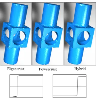
Figure 7 shows that the eigencrust is poor at capturing sharp corners, and the Powercrust algorithm is much better, but the hybrid algorithm is even more effective. Spectral partitioning labels power cells better than the original Pow-ercrust. The hybrid spectral Powercrust algorithm shares the Powercrust’s advantage of recovering sharp corners well, but it also shares its disadvantage of increasing the number of vertices many-fold. The number of vertices in each model is 4,100, 52,078, and 51,069, respectively.

3.5. Constructing Manifolds

An optional heuristic step searches for local topological ir-regularities that prevent the reconstructed surface from being a manifold, and makes the surface a manifold by relabeling selected tetrahedra frominsidetooutside.

Eigencrust Powercrust Hybrid

Figure 7: Reconstructions of a mechanical part by three algorithms. The eigencrust algorithm uses both eigenvec-tors, whereas the hybrid (spectral Powercrust) algorithm uses only the first.

These irregularities come in two types. First, consider any edge e of the Delaunay tetrahedralization T . The tetrahedra that have e for an edge form a ring around e. If the recon-structed surface is a manifold, there are three possibilities: the tetrahedra in the ring are alloutside, they are allinside, or the ring can be divided into a contiguous strand ofinside

tetrahedra and a contiguous strand ofoutsidetetrahedra. If the ring of tetrahedra around e do not follow any of these patterns—if there are two or more contiguous strands of in-sidetetrahedra in the ring—then we fix the irregularities by relabeling some of the tetrahedra frominsidetooutsideso that only one contiguous strand ofinsidetetrahedra survives. The surviving strand is chosen so that it contains theinside

tetrahedron that was assigned the largest absolute eigenvec-tor component during the second partitioning stage.

The second type of irregularity involves any point sample s in S. If the reconstructed surface is a manifold, then the tetrahedra that have s for a vertex are either alloutside, all

inside, or divided into one face-connected block ofoutside

tetrahedra and one face-connected block ofinsidetetrahedra. A topological irregularity at s may take the form of two in-sidetetrahedra that have s for a vertex, but are not connected to each other through a path of face-connectedinside tetrahe-dra all having s for a vertex. In this case, theinsidetetrahedra adjoining s can be divided into two or more face-connected components. Only one of theseinsidecomponents survives; we relabel the othersoutside. The surviving component is the one that contains a pole of s. (In the unlikely case that there are two such components, choose one arbitrarily.)

It is also possible to have two or more face-connected

components ofoutsidetetrahedra (and just one component ofinsidetetrahedra). Let W and X be two of them. We com-pute the shortest face-connected path from W to X , where the length of a path is defined to be the sum of the absolute eigenvector components of theinsidetetrahedra on the path. The tetrahedra on the shortest path are relabeledoutside.

These operations are repeated until no irregularity re-mains. The final surface is guaranteed to be a manifold. One can imagine that for a pathological model this proce-dure might whittle down the object to a few tetrahedra, but in practice it rarely takes an unjustifiably large bite out of an object.

3.6. Smoothing

Triangulated surfaces extracted from noisy models are bumpy. The final optional step is to use standard Lapla-cian smoothing [Her76] to remove the artifacts created by measurement errors in laser range finding, and to make the model more amenable to rendering and simulation. Lapla-cian smoothing visits each vertex in the triangulation in turn, and moves it to the centroid of its neighboring vertices. We performed five iterations of smoothing on the smoothed bunny and dragon in Figures 6 and 8.

4. Results

Our implementation uses our own Delaunay tetrahedraliza-tion software, and TRLAN, an implementatetrahedraliza-tion of the Lanc-zos algorithm by Kesheng Wu and Horst Simon of the Na-tional Energy Research Scientific Computing Center.

Figure 8 illustrates the performance of the spectral algo-rithm on the Stanford Dragon. The raw data exhibit random measurement errors and include natural outliers. Spectral reconstruction yields a watertight manifold surface, and re-moves all the outliers.

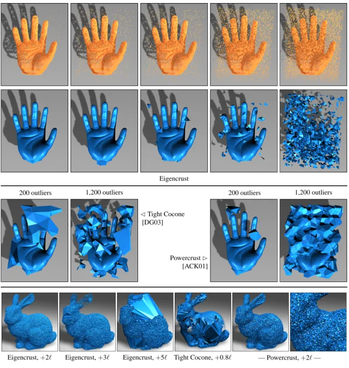
Figure 9 shows how several algorithms degrade as ran-domly generated outliers are added to the input data. Even 1,200 random outliers have no influence on the eigencrust except to affect how a hole at the base of the hand is patched. The Tight Cocone and Powercrust algorithms are incapaci-tated by relatively few outliers, although they correctly re-construct models without outliers.

The fourth row of Figure 9 shows the degradation of sev-eral algorithms as increasing amounts of random Gaussian noise are added to the point coordinates of the Stanford Bunny, which already includes measurement errors. The expression under each reconstruction is the variance of the Gaussian distribution used to produce additional noise in each coordinate, expressed in terms of the grid spacing` defined in Section 3.3. The eigencrust remains a genus zero manifold when the added noise has variance 2`, but begins to disintegrate as the measurement errors become notably larger than the resolution of the range data. With added noise of variance`, the Powercrust algorithm succeeds, but with variance 2`the structure is full of holes. (It is a watertight surface, but what it bounds is Swiss cheese.) The Tight

Co-Figure 8: Eigencrust reconstruction of the Stanford Dragon model from raw data. The point cloud (upper left) has many outliers, which are automatically omitted from the spectrally recovered surface. 1,769,513 input points; 11,660,147 tetra-hedra; 2,599,114 surface triangles; genus 1; 197 minutes reconstruction time.

cone algorithm can only cope with noise of less than 0.8` variance.

Figure 10 illustrates the three algorithms on a set of points densely sampled from the smooth splines of the Utah Teapot. The difficulties here are more subtle. The teapot’s spout pen-etrates the body deeply enough to create an ambiguity that neither the Powercrust nor Tight Cocone algorithm solves correctly. The spectral reconstruction algorithm treats the interior spout sample points as outliers, and correctly omits them from the eigencrust.

The spectral algorithm is not infallible. It occasionally creates unwanted handles—thirteen on the angel. The global eigenvector computation is slow. Tetrahedron-labeling algo-rithms do not reconstruct sharp corners well—observe how the teapot adjoins its spout. This problem can sometimes be overcome by labeling power cells rather than tetrahedra, at the cost of much larger model complexity. Either way, however, spectral surface reconstruction is remarkably ro-bust against noise, outliers, and undersampling.

Acknowledgments

We thank Chen Shen for rendering many of our models, and Nina Amenta and Tamal Dey for providing their sur-face reconstruction programs. This work was supported in part by the National Science Foundation under Awards ACI-9875170, CMS-9980063, and CCR-0204377, in part by the State of California under MICRO Award 02-055, and in part by generous support from Pixar Animation Studios, Intel Corporation, Sony Computer Entertainment America, and the Okawa Foundation.

References

[AB99] AMENTAN., BERNM.: Surface Reconstruc-tion by Voronoi Filtering. Discrete and Compu-tational Geometry 22 (1999), 481–504.

[ABK98] AMENTA N., BERN M., KAMVYSSELISM.: A New Voronoi-Based Surface Reconstruction Algorithm. In Computer Graphics (SIGGRAPH ’98 Proceedings) (July 1998), pp. 415–421. [ACDL02] AMENTA N., CHOI S., DEY T. K., LEEKHA

N.: A Simple Algorithm for Homeomorphic Surface Reconstruction. International Journal of Computational Geometry and Applications 12, 1–2 (2002), 125–141.

[ACK01] AMENTA N., CHOI S., KOLLURI R.: The Power Crust. In Proceedings of the Sixth Sym-posium on Solid Modeling (2001), Association for Computing Machinery, pp. 249–260. [AK00] AMENTAN., KOLLURIR.: Accurate and

Ef-ficient Unions of Balls. In Proceedings of the Sixteenth Annual Symposium on Computational Geometry (June 2000), Association for Com-puting Machinery, pp. 119–128.

[BMR∗99] BERNADINIF., MITTLEMANJ., RUSHMEIER

H., SILVAC., TAUBING.: The Ball-Pivoting Algorithm for Surface Reconstruction. IEEE Transactions on Visualization and Computer Graphics 5, 4 (Oct. 1999), 349–359.

[Boi84] BOISSONNAT J.-D.: Geometric Structures for Three-Dimensional Shape Reconstruction. ACM Transactions on Graphics 3 (Oct. 1984), 266–286.

[BTG95] BITTAR E., TSINGOS N., GASCUEL M.-P.: Automatic Reconstruction of Unstructured 3D Data: Combining Medial Axis and Implicit Sur-faces. Computer Graphics Forum 14, 3 (1995), 457–468.

[CBC∗01] CARRJ. C., BEATSONR. K., CHERRIEJ. B., MITCHELL T. J., FRIGHT W. R., MCCAL

-LUMB. C., EVANST. R.: Reconstruction and Representation of 3D Objects with Radial Basis Functions. In Computer Graphics (SIGGRAPH 2001 Proceedings) (Aug. 2001), pp. 67–76. [CL96] CURLESS B., LEVOY M.: A Volumetric

Method for Building Complex Models from Range Images. In Computer Graphics (SIG-GRAPH ’96 Proceedings) (1996), pp. 303–312. [DG03] DEY T. K., GOSWAMIS.: Tight Cocone: A Water-tight Surface Reconstructor. Journal of Computing and Information Science in Engi-neering 3, 4 (Dec. 2003), 302–307.

[DG04] DEY T. K., GOSWAMI S.: Provable Surface Reconstruction from Noisy Samples. In Pro-ceedings of the Twentieth Annual Symposium on Computational Geometry (Brooklyn, New York, June 2004), Association for Computing Machinery.

200 outliers 1,200 outliers 1,800 outliers 6,000 outliers 10,000 outliers

Eigencrust

200 outliers 1,200 outliers 200 outliers 1,200 outliers

CTight Cocone [DG03]

PowercrustB [ACK01]

Eigencrust,+2` Eigencrust,+3` Eigencrust,+5` Tight Cocone,+0.8` — Powercrust,+2`—

Figure 9: Top row: 25,626 noise-free points plus randomly generated outliers. Second row: eigencrust reconstructions of this model maintain their integrity to 1,200 outliers, then begin to degrade. Third row: other Delaunay-based algorithms degrade much earlier. Fourth row: Stanford Bunny reconstructions from raw data, with natural noise plus added random Gaussian noise. The amount of random noise is expressed as the variance of the Gaussian noise added to each point coordinate, in terms of the grid spacing`defined in Section 3.3. The eigencrust maintains its integrity with+2`added noise; all the other bunny reconstructions here exhibit serious failures.

Eigencrust Tight Cocone Eigencrust Powercrust Figure 10: Reconstructions from 253,859 points sampled on the Utah Teapot. The spout’s splines penetrate into the body of the teapot, causing difficulties for both the Powercrust and Tight Cocone algorithms. A cutaway view shows that Powercrust mislabels asoutsidea cluster of power cells where the spout enters the body. The spectral algorithm correctly identifies the same poles asinside.

[Fie73] FIEDLER M.: Algebraic Connectivity of Graphs. Czechoslovak Mathematical Journal 23, 98 (1973), 298–305.

[For92] FORTUNES.: Voronoi Diagrams and Delaunay Triangulations. In Computing in Euclidean Ge-ometry, Du D.-Z., Hwang F., (Eds.), vol. 1 of Lecture Notes Series on Computing. World Sci-entific, Singapore, 1992, pp. 193–233.

[Hal70] HALL K. M.: An r-Dimensional Quadratic Placement Algorithm. Management Science 11, 3 (1970), 219–229.

[HDD∗92] HOPPE H., DEROSET., DUCHAMP T., MC -DONALDJ., STUETZLEW.: Surface Recon-struction from Unorganized Points. In Com-puter Graphics (SIGGRAPH ’92 Proceedings) (1992), pp. 71–78.

[Her76] HERMANN L. R.: Laplacian-Isoparametric Grid Generation Scheme. Journal of the En-gineering Mechanics Division of the American Society of Civil Engineers 102 (Oct. 1976), 749–756.

[KBSS01] KOBBELT L. P., BOTSCH M., SCHWANECKE

U., SEIDEL H.-P.: Feature-Sensitive Sur-face Extraction from Volume Data. In Com-puter Graphics (SIGGRAPH 2001 Proceedings) (Aug. 2001), pp. 57–66.

[Lan50] LANCZOSC.: An Iteration Method for the So-lution of the Eigenvalue Problem of Linear Dif-ferential and Integral Operators. J. Res. Nat. Bur. Stand. 45 (1950), 255–282.

[LC87] LORENSEN W. E., CLINE H. E.: March-ing Cubes: A High Resolution 3D Surface Construction Algorithm. In Computer Graph-ics (SIGGRAPH ’87 Proceedings) (July 1987), pp. 163–170.

[LPC∗00] LEVOY M., PULLI K., CURLESS B., RUSINKIEWICZ S., KOLLER D., PEREIRA

L., GINZTON M., ANDERSON S., DAVISJ.,

GINSBERGJ., SHADEJ., FULKD.: The Digi-tal Michelangelo Project: 3D Scanning of Large Statues. In Computer Graphics (SIGGRAPH 2000 Proceedings) (2000), pp. 131–144. [OBA∗03] OHTAKEY., BELYAEVA., ALEXAM., TURK

G., SEIDEL H.-P.: Multi-Level Partition of Unity Implicits. ACM Transactions on Graphics 22, 3 (July 2003), 463–470.

[PSL90] POTHENA., SIMONH. D., LIOU K.-P.: Par-titioning Sparse Matrices with Eigenvectors of Graphs. SIAM Journal on Matrix Analysis and Applications 11, 3 (July 1990), 430–452. [SM00] SHIJ., MALIKJ.: Normalized Cuts and Image

Segmentation. IEEE Transactions on Pattern Analysis and Machine Intelligence 22, 8 (Aug. 2000), 888–905.

[TL94] TURK G., LEVOY M.: Zippered Poly-gon Meshes from Range Images. In Com-puter Graphics (SIGGRAPH ’94 Proceedings) (1994), pp. 311–318.

[TO99] TURKG., O’BRIENJ.: Shape Transformation Using Variational Implicit Functions. In Com-puter Graphics (SIGGRAPH ’99 Proceedings) (1999), pp. 335–342.

[Whi98] WHITAKERR. T.: A Level-Set Approach to 3D Reconstruction from Range Data. International Journal of Computer Vision 29, 3 (1998), 203– 231.

[YS01] YU S. X., SHI J.: Understanding Popout through Repulsion. In IEEE Conference on Computer Vision and Pattern Recognition (Dec. 2001).

[ZOF01] ZHAO H.-K., OSHER S., FEDKIWR.: Fast Surface Reconstruction Using the Level Set Method. In First IEEE Workshop on Variational and Level Set Methods (2001), pp. 194–202.