Understanding Coupling of Global and Diffuse Solar Radiation with Climatic Variability

Graduate Theses, Dissertations, and Problem Reports 2016

Understanding Coupling of Global and Diffuse Solar Radiation

Understanding Coupling of Global and Diffuse Solar Radiation

with Climatic Variability

with Climatic Variability

Follow this and additional works at: https://researchrepository.wvu.edu/etd Recommended Citation

Recommended Citation

Hamdan, Lubna, "Understanding Coupling of Global and Diffuse Solar Radiation with Climatic Variability" (2016). Graduate Theses, Dissertations, and Problem Reports. 5742.

https://researchrepository.wvu.edu/etd/5742

This Dissertation is protected by copyright and/or related rights. It has been brought to you by the The Research Repository @ WVU with permission from the rights-holder(s). You are free to use this Dissertation in any way that is permitted by the copyright and related rights legislation that applies to your use. For other uses you must obtain permission from the rights-holder(s) directly, unless additional rights are indicated by a Creative Commons license in the record and/ or on the work itself. This Dissertation has been accepted for inclusion in WVU Graduate Theses, Dissertations, and Problem Reports collection by an authorized administrator of The Research Repository @ WVU. For more information, please contact [email protected].

UNDERSTANDING COUPLING OF GLOBAL AND DIFFUSE SOLAR RADIATION WITH CLIMATIC VARIABILITY

Lubna Hamdan

Dissertation submitted to the

Statler College of Engineering and Mineral Resources at West Virginia University

in partial fulfillment of the requirements for the degree of

Doctor of Philosophy in

Industrial Engineering

Majid Jaridi, Ph.D., Chair Antarpreet Jutla, Ph.D., Co-chair

E. James Harner, Ph.D. Feng Yang, Ph.D. Ashish Nimbarte, Ph.D. Robert Mnatsakanov, Ph.D.

Department of Industrial and Management Systems Engineering

Morgantown, West Virginia 2016

Keywords: Global Radiation, Diffuse Radiation, Atmospheric parameters, Regression Analysis, Multivariate Analysis, Prediction Models

Abstract

UNDERSTANDING COUPLING OF GLOBAL AND DIFFUSE SOLAR RADIATION WITH CLIMATIC VARIABILITY

Lubna Hamdan

Global solar radiation data is very important for wide variety of applications and scientific studies. However, this data is not readily available because of the cost of measuring equipment and the tedious maintenance and calibration requirements. Wide variety of models have been introduced by researchers to estimate and/or predict the global solar radiations and its components (direct and diffuse radiation) using other readily obtainable atmospheric parameters. The goal of this research is to understand the coupling of global and diffuse solar radiation with climatic variability, by investigating the relationships between these radiations and atmospheric parameters. For this purpose, we applied multilinear regression analysis on the data of National Solar Radiation Database 1991- 2010 Update.

The analysis showed that the main atmospheric parameters that affect the amount of global radiation received on earth’s surface are cloud cover and relative humidity. Global radiation correlates negatively with both variables. Linear models are excellent approximations for the relationship between atmospheric parameters and global radiation. A linear model with the predictors total cloud cover, relative humidity, and extraterrestrial radiation is able to explain around 98% of the variability in global radiation.

For diffuse radiation, the analysis showed that the main atmospheric parameters that affect the amount received on earth’s surface are cloud cover and aerosol optical depth. Diffuse radiation correlates positively with both variables. Linear models are very good approximations for the relationship between atmospheric parameters and diffuse radiation. A linear model with the predictors total cloud cover, aerosol optical depth, and extraterrestrial radiation is able to explain around 91% of the variability in diffuse radiation. Prediction analysis showed that the linear models we fitted were able to predict diffuse radiation with efficiency of test adjusted R2 values equal to 0.93, using the data of total cloud cover, aerosol optical depth, relative humidity and extraterrestrial radiation. However, for prediction purposes, using nonlinear terms or nonlinear models might enhance the prediction of diffuse radiation.

iii DEDICATION

I dedicate this work to my husband Nader and to my family. Their support, encouragement, and prayers helped me overcome the difficulties and eased the pressure that I faced

iv

ACKNOWLEDGMENTS

I would like to express my sincere appreciation to my advisor, Dr. Majid Jaridi, for his guidance, continued help, support, and encouragement, and for having confidence in me. I would like to thank my co-advisor, Dr. Antarpreet Jutla, for his guidance, help and support throughout my research. I would like to thank Dr. E. James Harner for guiding me throughout the statistical analysis of my research. I was lucky to work with all of them and learn from their experience and skills in the field of research.

I would like to thank my committee members: Dr. Feng Yang, Dr. Ashish Nimbarte, and Dr. Robert Mnatsakanov for being my committee members and accepting the heavy task of going through my dissertation. I am grateful to all my professors, my colleagues, and the staff of Industrial Engineering Department for their help and support.

Finally, my thanks and appreciation are to my husband, my family, and my friends for their support, help, and encouragement. I am blessed to have such a supportive and loving family and friends.

v

Table of Contents

Abstract ... ii

DEDICATION ... iii

ACKNOWLEDGMENTS ... iv

LIST OF FIGURES ... vii

LIST OF TABLES ... x

NOMENCLATURE ... xi

CHAPTER 1: INTRODUCTION ... 1

CHAPTER 2: LITERATURE REVIEW ... 4

2.1 Global Radiation ... 4

2.2 Diffuse Radiation ... 18

CHAPTER 3: PROBLEM STATEMENT AND PROPOSED APPROACH ... 23

3.1 Approach ... 23

3.2 Data ... 24

3.2.1 Source of data... 24

3.2.2 Data files ... 27

3.2.3 Data testing ... 30

CHAPTER 4: CLOBAL RADIATION ... 32

4.1 Preliminary Analysis... 32

4.2 Multiple Linear Regression Analysis ... 33

4.2.1 Models with Clearness Index (K) response ... 34

4.2.2 Models with log (H) response ... 41

4.2.3 Models with H response ... 46

4.3 Prediction Analysis ... 50

4.4 Discussion and Conclusions ... 53

CHAPTER 5: DIFFUSE RADIATION ... 57

5.1 Preliminary Analysis... 57

5.2.1 Models with Diffuse Fraction (Kd) Response ... 58

5.2.2 Models with Diffuse Radiation (Hd) Response ... 66

5.2.3 Models with log (Hd) Response ... 73

vi

5.4 Discussion and Conclusions ... 78

CHAPTER 6: COMPLEMENTARY ANALYSES... 81

6.1 Regularized Regression ... 81

6.2 Autoregressive Analysis for the Residuals ... 83

6.3 Leave Out One Station Cross Validation ... 86

CHAPTER 7: GENERAL CONCLUSIONS AND FUTURE WORK ... 88

7.1 General Conclusions ... 88

7.2 Technical Contributions ... 89

7.3 Impact on Energy Industry. ... 89

7.4 Future Work ... 89

APPENDIX ... 91

vii

LIST OF FIGURES

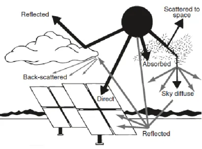
Figure 1.1: Solar radiation components segregated by the atmosphere and surface---2

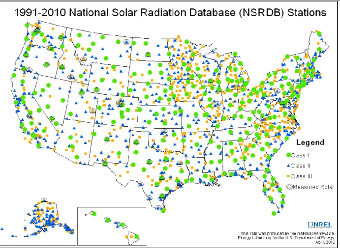
Figure 3.1: NSRDB 1991-2010 stations with their classification---25

Figure 3.2: Daily Statistical File of NSRDB 1991-2010 for Albuquerque, New Mexico---27

Figure 3.3: Pictorial description for cloud cover derivation---29

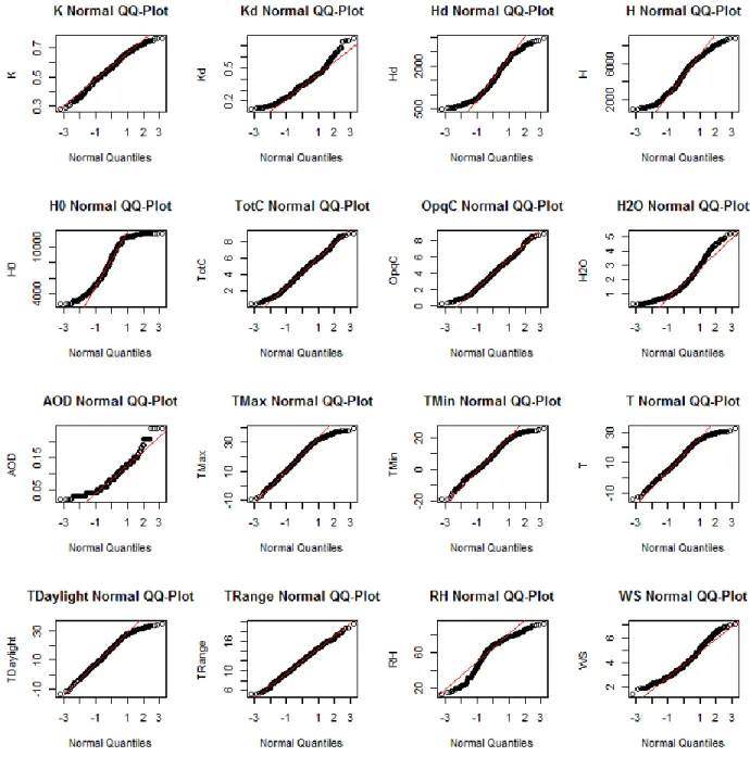
Figure 3.4: Normal QQ plots for solar radiations and atmospheric parameters data---30

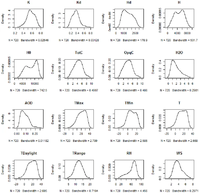
Figure 3.5: Probability distributions for solar radiations and atmospheric parameters---31

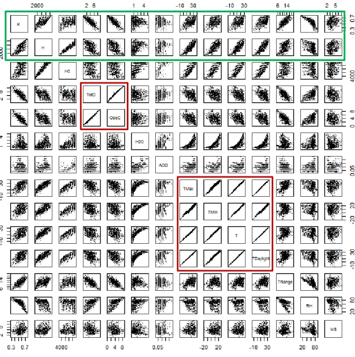
Figure 4.1: The scatterplot matrix of global radiation and atmospheric parameters---32

Figure 4.2: The Correlation matrix of global radiation and atmospheric parameters---33

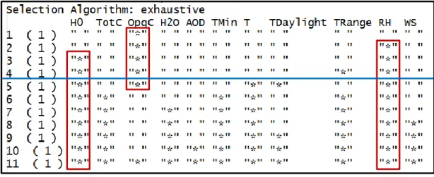
Figure 4.3: Best subset selection results for the models with K response---36

Figure 4.4: Best model of K response subsets based on adjusted R2_{, Cp and BIC selection---36}

Figure 4.5: The results of fitting K against OpqC, RH, H0, and TRange variables---37

Figure 4.6: Diagnostic plots for model (4.6). A- Linearity and constant variance of 𝜖 test. B- Normality test (𝜖~𝑁(0, 𝜎2). C- Outliers test. D- High leverage points test---38

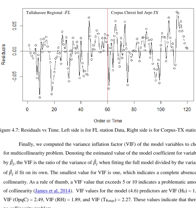
Figure 4.7: Residuals vs Time. Left side is for FL station Data, Right side is for Corpus-TX station---40

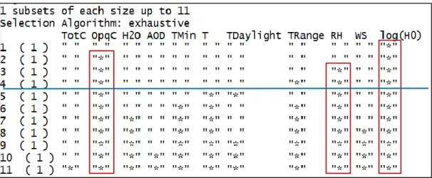
Figure 4.8: Best subset selection results for the models with log (H) response---42

Figure 4.9: Best log (H) response model of best subsets based on adjusted R2, Cp and BIC selection---42

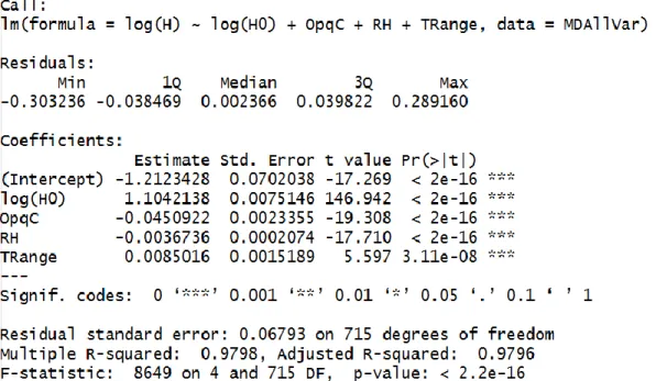
Figure 4.10: The results of fitting log (H) against log (H0), OpqC, RH, and TRange ---43

Figure 4.11: Diagnostic plots for model (4.11). A- Linearity and constant variance of 𝜖 test. B- Normality test (𝜖~𝑁(0, 𝜎2). C- Outliers test. D- High leverage points test---44

Figure 4.12: The results of fitting log (H) against offset (log (H0)), OpqC, RH, and TRange ---45

Figure 4.13: Best subset selection results for the models with H response---46

Figure 4.14: Best model of H response subsets based on adjusted R2, Cp and BIC selection---47

viii

Figure 4.16: Diagnostic plots for model (4.13). A- Linearity and constant variance of ϵ test.

B- Normality test (ϵ~N (0, σ^2). C- Outliers test. D- High leverage points test---48

Figure 4.17: Residuals vs Time for H response model. Left side is for FL station Data, Right side is for Corpus-TX station---49

Figure 5.1: The scatterplots and correlations of average daily diffuse radiation and daily diffuse fraction with atmospheric parameters---57

Figure 5.2: Best subset selection results for the Kd response models---58

Figure 5.3: Best model of Kd response subsets based on adjusted R2, Cp and BIC selection---59

Figure 5.4: Best subset selection results for the Kd response models without predictor K---59

Figure 5.5: Best Kd response model of the subsets without K predictor, based on adjusted R2, Cp and BIC selection---60

Figure 5.6: The results of fitting Kd against K, AOD, and RH variables---62

Figure 5.7: Diagnostic plots for model (5.1). A- Linearity and constant variance of 𝜖 test. B- Normality test (𝜖~𝑁(0, 𝜎2_{). C- Outliers test. D- High leverage points test---63}

Figure 5.8: Residuals vs Time for model (5.1). Left is for FL station Data, right is for Corpus-TX---63

Figure 5.9: The results of fitting Kd against OpqC, AOD, H0, and RH variables---65

Figure 5.10: Diagnostic plots for model (5.3) ---65

Figure 5.11: Residuals vs Time for model (5.3) ---66

Figure 5.12: Best subset selection results for the models with Hd response---67

Figure 5.13: Best model of Hd response subsets based on adjusted R2, Cp and BIC selection----67

Figure 5.14: The results of fitting Hd against H0, H, AOD, and TotC---68

Figure 5.15: Diagnostic plots for model (5.14). A- Linearity and constant variance of 𝜖 test. B- Normality test (𝜖~𝑁(0, 𝜎2_{). C- Outliers test. D- High leverage points test---69}

Figure 5.16: Residuals vs Time for model (5.4). Left side is FL station Data, Right side is Corpus-TX station---70

Figure 5.17: Best subset selection results for Hd response models that exclude predictor H0 ----70

ix

Figure 5.19: Best subset selection results for Hd response models that exclude predictor H---72

Figure 5.20: The results of fitting Hd against H0, AOD, TotC, and RH---72

Figure 5.21: Best subset selection results for log (Hd) response models---74

Figure 5.22: The results of fitting log (Hd) against log (H0), AOD, TotC, and RH---74

Figure 5.23: Diagnostic plots for model (5.8) ---75

Figure 5.24: Residuals vs Time for model (5.8). Left side is FL station Data, Right side is Corpus-TX station---75

Figure 6.1: Autoregressive function for residuals of model (4.12) ---85

x

LIST OF TABLES

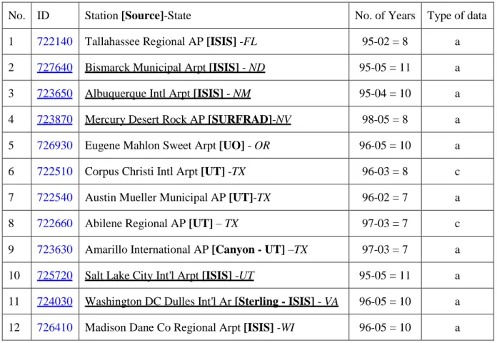
Table 3.1: First class stations that have both measured diffusion and globalradiation---26

Table 3.2: Variables used in the analysis with their definitions and measure units---28

Table 4.1: The test data used to evaluate models performance---51

Table 4.2: The accuracy of global models based on the statistical error tests---52

Table 4.3: The most important parameters in descending order for the major global models---54

Table 5.1: The accuracy of diffuse models based on the statistical error tests---76

Table 5.2: The most important parameters in descending order for the major diffuse models---79

Table 6.1: The coefficients and performance of MLR models, the lasso (𝝀=3.4) and ridge regression (𝝀=192.0) for global radiation---84

Table 6.2: The coefficients and performance of MLR models, the lasso (𝝀=.06) and ridge regression (𝝀=57.86) for diffuse radiation---84

Table 6.3: LOOSCV for model (6.3); station name represents the station used in testing the model---86

Table 6.2: LOOSCV for model (6.4); station name represents the station used in testing the model---87

xi

NOMENCLATURE

AOD Monthly average of broadband aerosol optical depth (unitless) C Cloud cover in oktas or tenths

Cp Mallow’s Cp

d Hourly diffuse fraction

E Mean evaporation (cm)

F Time of sunshine expressed in the greatest possible time of sunshine (sunshine fraction) 𝐹̅ Mean value of sunshine fraction

𝑓_{𝑐𝑙𝑒𝑎𝑟} Time fraction that no significant clouds block the sun

h Elevation (m)

H Monthly average of the daily global solar radiation on a horizontal surface (Wh/m2) 𝐻𝑏 Monthly average of the daily beam radiation on a horizontal surface (Wh/m2) 𝐻𝑑

H0 Monthly average of daily extraterrestrial solar radiation on a horizontal surface (Wh/m2) 𝐻𝑐𝑙𝑒𝑎𝑟 Monthly average of daily clear sky horizontal surface radiation (J/m2)

𝐻2𝑂 Monthly average of precipitable water (cm) 𝐼𝐷 Diffuse horizontal irradiation (W/m2) 𝐼_𝐺 Global horizontal irradiation (W/m2)

𝐼_𝐺𝐶 Clear-sky global horizontal irradiation (W/m2) IN Normal terrestrial beam solar irradiation (W/m2) ION Normal extraterrestrial solar irradiation (W/m2) 𝐾 Monthly average of clearness index (𝐾 = 𝐻

𝐻0 )

𝐾𝑐𝑙𝑒𝑎𝑟 Monthly average of clear sky clearness index (𝐾𝑐𝑙𝑒𝑎𝑟= 𝐻𝑐𝑙𝑒𝑎𝑟

𝐻0 )

𝐾_𝑑 Monthly average of diffuse fraction (𝐻𝐷

𝐻) 𝐾𝑡 Daily clearness index

xii 𝑛 Number of observations

𝑂𝑝𝑞𝐶 Monthly average of Opaque sky cover (tenths) 𝑝 Number of predictors in a model

Q Total radiation income during a day (MJ/m2₎

Qclear Radiation income that corresponds to a perfectly clear sky day (MJ/m2) Q0 Extraterrestrial radiation on a horizontal surface during the day (MJ/m2) R2 Coefficient of determination

RH Monthly average of relative humidity (%) S Monthly average daily bright sunshine hours

S0 Maximum possible monthly average daily sunshine hours or the day length ST Mean soil temperature (°C)

T Monthly average of temperature or mean temperature (°C) TMax Monthly average of maximum temperature (°C)

TMin Monthly average of minimum temperature (°C) TDaylight Monthly average of daylight temperature (°C) TRange Monthly average of temperature range (°C) 𝑇𝑜𝑡𝐶 Monthly average of total sky cover (tenths) ∆𝑇 Daily temperature range

WS Monthly average of wind speed (m/s) 𝑥_𝑖𝑗 ith observation for the variable j

𝑦_𝑖 ith measured response

𝑦̂𝑖 ith fitted or predicted response

𝑦̅ The average or mean of the responses Y (𝑦1… 𝑦𝑛)

∝ Solar elevation (the angle between the horizon and the center of the sun's disc) (radian or (°)).

𝛿 Solar declination (the angle between the rays of the Sun and the plane of the Earth's equator) (radian or (°))

xiii

𝜃𝑧 Solar zenith angle (the angle between the vertical and center of the sun's disc) (radian or (°))

𝝀 Tuning parameter for ridge regression and the lasso 𝜎̂2 _{Estimated variance of errors}

AR Autoregressive

BIC Bayesian Information Criterion

ISIS Integrated Surface Irradiance Study network LOOSCV Leave Out One Station Cross Validation

MAPE Mean Absolute Percentage Error

MBE Mean Bias Error

MLR Multiple Linear Regression

MPE Mean Percentage Error

MSE Mean Squared Error

NCDC National Climatic Data Center

NOAA National Oceanic and Atmospheric Administration

NREL National Renewable Energy Laboratory

NSRDB National Solar Radiation Database

RMSE Root Mean Squared Error

RSS Residual Sum of Squares

SURFRAD Surface Radiation Budget Measurement network

TSS Total Sum of Squares

UO University of Oregon Solar Radiation Monitoring Laboratory Network USAF United States Air Force

UT University of Texas Solar Energy Laboratory

1

CHAPTER 1: INTRODUCTION

Solar radiation arriving the earth’s surface is the most fundamental renewable energy source in nature. It sustains the biosphere and drives its self-organization; it also drives many of earth’s physical processes. Time and space dependent solar radiation changes the distribution of temperature, moisture, clouds, and precipitation as well as the pattern of atmospheric and oceanic circulations (Zhang et al, 2013). In addition, solar radiation, as a source of renewable energy, can play a key role in de-carbonizing the global economy since it is abundant and harnessing it has little adverse environmental impact. There is hardly any pollution in the form of exhaust fumes or even noise associated with conventional solar energy generation technologies. Accordingly, knowing the amount of solar radiation that reaches the surface of the earth is very important for a wide range of applications in engineering, meteorology, agricultural sciences, health sector, and natural sciences. Some examples of applications that use the solar radiation data at ground level include air conditioning and cooling systems in architecture and building design, solar heating system design and use, solar power generation and solar powered car races. As well, weather and climate prediction models, evaporation and irrigation, calculation of water requirements for crops, monitoring plant growth, and disease control and skin cancer research (Badescu, 2008).

Solar radiation reaching the earth’s surface is time and space dependent. A summary of the parameters affecting solar irradiation is as follows (Ertekin and Yaldiz, 1999):

 Astronomical factors (solar constant, earth-sun distance, solar declination and hour angle)

 Geographical factors (latitude, longitude and elevation of the site)

 Geometrical factors (azimuth angle of the surface, tilt angle of the surface, sun elevation angle, sun azimuth angle)

 Physical factors (water vapor content, scattering of dust and particulates, scattering of air molecules such as O2, N2, CO2, O3, etc.)

 Meteorological factors (effects of cloudiness, reflection of the environs)

We can calculate solar radiation incident on a horizontal plane outside the atmosphere (extraterrestrial radiation) at any point, using astronomical, geometrical, and geographical parameters of the site at a specific time. The details are in (Duffie and Beckman, 2013). However,

2

radiation incident on the earth’s surface, at some point, is random in nature due to the effect of physical and meteorological factors. Namely, as extraterrestrial radiation traverses the atmosphere, gases, dust, water vapor, and clouds within the atmosphere reflect, scatter and absorb the solar radiation at different wavelengths.

Due to the interaction between solar radiation and atmosphere constituents, we have two components of solar radiation incident on a horizontal plane at earth’s surface. The first component is diffuse sky radiation or simply diffuse radiation, which results from scattered photons (mostly at short wavelengths). The remaining unabsorbed and unscattered photons constitute the second component, direct beam radiation, which is responsible for the casting of shadows. The total solar radiation flux resulting from diffuse and beam radiations on a horizontal surface is called total or global solar radiation. The difference between global solar radiation at the top of the atmosphere and its corresponding value at the ground level is the amount of radiation that atmosphere has absorbed or reflected away. On average, earth reflects about 29% of the incident solar radiation. For a tilted surface, beside the beam and diffuse radiations, there is a third component, which is the radiation, reflected from the ground, see Figure 1.1 (Gueymard and Myers, 2008).

Pyrheliometer is the instrument that measures the direct beam radiation. Pyrheliometers have a narrow aperture (generally between 5◦ and 6◦ total solid angle), admitting only beam radiation with some inadvertent circumsolar contribution from the Sun’s aureole. However, the

3

aperture excludes all diffuse radiation from the sky. Pyrheliometers must be pointed at sun and track it through the day. Their sensor should be always normal to the direct beam. Pyranometer is the instrument that measures the global radiation or the diffuse sky radiation. Pyranometers have a 180◦ (2π steradian) field of view. To measure diffuse radiation using the pyranometer, beam radiation is blocked out with a disk or ball placed over the instrument and in the path of the direct beam. The blocking device must track the sun through the day (Gueymard and Myers, 2008).

Unfortunately, in spite of the importance of solar radiation measurements, these data are not readily available for many developing countries because of the cost of measuring equipment and the tedious maintenance and calibration requirements (Al-Mostafa et al, 2014). Even all over the world, weather stations measuring solar radiation are very sparse. For example, in USA, 1% of meteorological stations are recording solar radiation. In China, only 122 stations are recording solar radiation out of more than 2000 stations have records of meteorological data. In Australia, the ratio of weather stations recording global solar radiation to those recording air temperatures was approximately 16 to 845 in 2006. Worldwide, the ratio of stations recording solar radiation to those recording temperature is about 1:500 (Chen and Li, 2012). Because of the limited coverage of solar radiation measuring networks, there is a need for developing solar radiation models able to estimate the data required for solar-energy applications. Since 1920’s a number of methods and correlations have been developed to estimate global solar radiation, based on the more readily available meteorological data (sunshine duration, cloud cover, temperature...etc.) at the majority of weather stations. However, these models depend on the local geographical, physical, and meteorological factors of the site of interest. Next, we present a brief review for some of these models.

4

CHAPTER 2: LITERATURE REVIEW

2.1 Global Radiation

Angstrom(1924) developed the first basic model for estimating global solar radiation when he introduced his famous empirical equation, which relates the global solar radiation on a horizontal surface, scaled by clear-sky global radiation, to the sunshine fraction:

𝑄

𝑄𝑐𝑙𝑒𝑎𝑟

= 𝑎 + (1 − 𝑎)𝐹

where Q is the total radiation income during a day (MJ/m2/day), Qclear is the radiation income

that corresponds to a perfectly clear sky day (MJ/m2/day), F is the time of sunshine expressed in the greatest possible time of sunshine, and 𝒂 is empirical coefficient. Angstrom obtained the value 𝛼 = 0.25 for Stockholm.

Prescott (1940) suggested using a modified form of Angstrom equation (Eq. (2.1)), since it is difficult to estimate Qclear, The modification is to use the radiation incident on a horizontal surface with transparent atmosphere (extraterrestrial radiation) instead of cloudless day:

𝑄

𝑄0

= 𝑎 + 𝑏𝐹

where Q0 is the extraterrestrial radiation on a horizontal surface during the day (MJ/m2/day), “a”

and “b” are coefficients that depend on the location.

Equation (2.2) is known as Angstrom-Prescott equation or model.

Hereafter, hundreds of articles in the literature introduced new models and improvements on the existing models, including the techniques used, to improve solar radiation estimation using readily available meteorological variables. Next, is a selection of these models presented in chronological order.

Black et al. (1954) used data collected from 32 stations around the world to estimate the coefficients of Angstrom-Prescott equation (Eq. (2.2)). They obtained the following general equation (at least within the range of latitudes studied) for predicting solar radiation from sunshine duration:

5

𝐻

𝐻0

= 0.23 + 0.48

𝑆

𝑆0

(2.3)

where H is the monthly average of the daily global solar radiation on a horizontal surface (MJ/m2_{/day), H}

0 is monthly average of daily total insolation on an extraterrestrial horizontal

surface. S is the monthly average daily bright sunshine hours and S0 is the maximum possible

monthly average daily sunshine hours or the day length (S/S0 = F in Equations (2.1) and (2.2)). However, they pointed out that there are errors in the data they did not consider: the different periods of collection for the stations and the different instruments used in different countries.

Rietveld (1978) examined several published values of Angstrom-Prescott coefficients and found that (a) is related linearly with 𝑭̅(the mean value of fraction of sunshine) and (b) is related hyperbolically with 𝐹̅ (b∝ 1/𝐹̅). His analysis showed that the use of these relationships to establish values of a and b provides more accurate estimates of radiation, from sunshine data, than does

Black et al. (1954) method or any extrapolated use of existing formulae.

Kasten and Czeplak (1980) investigated the dependence of total solar and terrestrial radiation fluxes at the earth surface on cloud amount and cloud type. They used 10 years of hourly data of solar and terrestrial radiations and of cloud amount and type. In their analysis, they used solar elevation (the angle between the horizon and the center of the sun's disc) as a parameter instead of hour of the day.

Wahab (1993) derived a quadratic form of Angstrom-Prescott equation, based on a simple model relating global solar radiation to cloud amount and transmissivity, ground albedo, and atmospheric backscatter (Davies and McKay, 1989). Abdel Wahab obtained the following equation, with “c” coefficient always negative:

𝐻 𝐻₀

= 𝑎 + 𝑏

+ 𝑐 (

)

Gueymard et al. (1995) criticized Wahab (1993) paper for the confusion between Angstrom equation (Eq. (2.1)) and Angstrom-Prescott equation (Eq. (2.2)), where Abdel Wahab analysis would be valid if he used Qclear instead of Q0, since he made the derivation based on Angstrom equation. Furthermore, they pointed out a number of errors in the paper, which preclude its use in actual solar radiation calculations. In addition, they criticized the interpretation of other

6

researchers for Rietveld model (1978), where they used F(the monthly average of daily sunshine fraction) instead of 𝑭̅ (the yearly average of daily sunshine fraction) to estimate the coefficients in Angstrom-Prescott equation. Moreover, Gueymard et al. emphasized that Angstrom-Prescott model has received considerable attention, yet it is still highly empirical. They advised to concentrate on improving original Angstrom model (Eq. (2.1)) by explicitly relating its coefficients to climatological variables.

Ododo et al. (1996) correlated global solar radiation with cloud cover and sunshine duration fraction using the data of three Nigerian stations. They used the following relation to predict global solar radiation:

𝐻 𝐻0

= 𝑏

+ 𝑏

+ 𝑏

𝐶 + 𝑏

𝐶

(2.5)

where C is the cloud cover in oktas. They obtained an excellent fit for one station and satisfactory results for the others.

Sen (1998) used theory of fuzzy sets to model solar irradiation and sunshine duration. He used a fuzzy logic algorithm for estimating the solar irradiation from sunshine duration measurements. The fuzzy model used does not provide an equation but can adjust itself to any type of linear or nonlinear form through fuzzy subsets of linguistic solar irradiation and sunshine duration variables. Sen believed that this method is suitable because solar radiation is a random process. He applied this method on some stations in the western part of Turkey. However, fuzzy logic algorithm may give better estimations, but it does not give physical interpretations for the results as regression analysis does.

Ertekin and Yaldiz (1999) used multiple linear regression models to estimate the monthly average daily global radiation for Antalya, Turkey using nine different variables. The variables are extraterrestrial radiation, solar declination, ratio of sunshine duration, mean relative humidity, mean temperature, mean soil temperature, mean cloudiness, mean precipitation and mean evaporation. From these variables they constructed 511 equations and found that the best model is the one which contains the nine variables at r = 0.99861.

7

𝐻 = −13.08 + 0.386𝐻₀+ .0902𝛿 + 0.2254𝑅𝐻 + 11.59 𝑆

𝑆0− 0.034𝑇 − 0.251𝑆𝑇 − 0.977𝐶 −

0.0072𝐻₂𝑂 + 0.2373𝐸 (2.6)

where 𝜹 is solar declination (the angle between the rays of the Sun and the plane of the Earth's equator) (°), RH is mean relative humidity (%), T is mean temperature (°C), ST is mean soil temperature (°C), 𝑪 is mean cloudiness (1-10), 𝑯_𝟐𝑶 is mean precipitation (cm), and E is mean evaporation (cm).

However, they had excellent values of correlation coefficient (r), at least for one model of each kind. The values started from r = 0.98447 using one variable equation, to r = 0.99860 using eight variables. Adding more variables did not give substantial improvement in radiation predictions since some variables are dependent on each other.

Suehrcke (2000) mentioned that the cloud transmittance depends on the radiation average. Hence, it is not constant as assumed by Angstrom’s equation, which suggests a non-linear sunshine-radiation relationship. Suehrcke used the properties of instantaneous solar radiation to derive a non-linear sunshine-radiation relationship free from empirical parameters, namely:

𝑓_{𝑐𝑙𝑒𝑎𝑟} = ( 𝐾 𝐾𝑐𝑙𝑒𝑎𝑟) 2 = ( 𝐻 𝐻𝑐𝑙𝑒𝑎𝑟) 2 (2.7)

where 𝒇_{𝒄𝒍𝒆𝒂𝒓} is time fraction that no significant clouds block the sun, 𝑯_{𝒄𝒍𝒆𝒂𝒓} is monthly average of daily clear sky horizontal surface radiation (J/m2), 𝑲 is monthly average daily clearness index (𝑲 = 𝑯

𝑯_𝟎 ) and 𝑲𝒄𝒍𝒆𝒂𝒓 is monthly average clear sky clearness index (𝑲𝒄𝒍𝒆𝒂𝒓= 𝑯_{𝒄𝒍𝒆𝒂𝒓}

𝑯𝟎

)

Suehrcke believes that Equation (2.7) may be universally valid and Angstrom–Prescott equation is a local (linear) approximation of his equation.

Ertekin and Yaldiz (2000) validated 26 models, available to predict the monthly average daily global radiation on a horizontal surface, using an independent data set for Antalaya Turkey. The models include linear, quadratic, third order polynomial and exponential equations. In addition, the models have different climatological and geographic parameters. Their analysis showed that the third order polynomial of Angstrom-Prescott type is the most accurate model:

8 𝐻 𝐻0

= 𝑎 + 𝑏

+ 𝑐 (

)

+ 𝑑 (

)

Muneer and Gul (2000) evaluated the performance of Page radiation model, which combines clouds and sunshine data to predict solar radiation, against two models developed by the authors. The first model is Meteorological Radiation Model, which uses hourly dry and wet bulb temperatures, and sunshine fraction to estimate hourly global, beam and diffuse irradiation. The second is Cloud Cover Radiation Model, which uses the hourly data of cloud amount to predict solar radiation. For the evaluation, they used data from UK sites. The analysis showed that Page model performs with maximum efficiency under overcast conditions and the Meteorological Radiation model gives the best results under clear skies. For intermediate conditions, both the Meteorological and Cloud Cover models are capable of generating quality data.

Driesse and Thevenard (2002) tested Suehrcke’s equation (Eq. (2.7)) for the calculation of monthly average daily radiation on a horizontal surface. They used 70,000 measured monthly sunshine and radiation data from nearly 700 sites compiled by the World Radiation Data Center. They also compared the performance of Suehrcke’s model with Angstrom-Prescott Model (Eq. (2.2)). They concluded that Suehrcke’s equation accounts adequately for the sunshine–radiation relationship on an average sense. However, the predictive capabilities of Suehrcke model are actually roughly equivalent to those of Angstrom-Prescott model when the peculiarities of local climatic conditions are not considered.

Yorukoglu and Celik (2006) conducted a literature survey and showed that researchers investigate either the goodness of the Angstrom–Prescott equation type model itself or the goodness of the estimation of global solar radiation. If the former is the objective, then the statistical analysis should be based on the variables H/H0 and S/S0. If the investigation was for goodness of estimation, then the statistical analysis should be based on 𝑯_𝒄 and 𝑯_𝒎 (calculated daily solar radiation vs. measured daily solar radiation). They showed that these two data sets are apt to be confused, where some researcher use 𝐻𝑐 and 𝐻𝑚 to investigate the goodness of the model or vice versa set. In addition, the authors compared five different Angstrom-Prescott type models (linear, quadratic, cubic, logarithmic and exponential) based on six years of measured hourly global solar radiation data. The analysis showed that amongst the five different models the Angstrom–Prescott equation, the quadratic and the cubic models are the best. Even though the

9

cubic model has slightly better performance than Angstrom–Prescott model (the simplest one), the advantage of the cubic model may be abandoned in return for a simpler model with half of the parameters.

Ertekin and Evrendilek (2007) compared the performance of eighteen empirical models in linear, quadratic, cubic, logarithmic, exponential and hybrid forms using only sunshine hours, latitude, and altitude. The models to estimate monthly average daily global solar radiation on a horizontal surface for 159 weather stations in Turkey. They found that the best models are a linear model (Angstrom type equation) with the coefficients that depend on the altitude and S/So and a hybrid model (quadratic with coefficients that depend on latitude and altitude). In addition, they generated spatial variability maps of global solar radiation on a 500 m x 500 m grid using the data of the 159 weather stations. However, they have values for R2adj greater than R2 !

Mellit et al. (2007) developed a new approach for predicting and modelling of daily total solar radiation data from sunshine duration and air temperature. They used an Adaptive Neuro-Fuzzy Inference Scheme (ANFIS) model. They built the simulation model in Matlab, using ten-year database of daily sunshine duration, ambient temperature and total solar radiation data. They validated the model with unknown data and showed that its estimations were excellent. Compared with other Adaptive Neuro Network models, their model was the best and the faster. This paper used simulation technique instead of regression analysis.

Younes and Muneer (2007) compared seven solar radiation models based on cloud information. These models are M1: Kasten and Czeplak (1980) model, represented in the following equations: 𝐼_𝐺𝐶 = 910𝑠𝑖𝑛 ∝ −30 (2.9) 𝐼𝐺 𝐼𝐺𝐶 = 1 − 0.75 ( 𝐶 8) 3.4 (2.10) 𝐼𝐷 𝐼𝐺 = 0.3 + 0.7 ( 𝐶 8) 2 (2.11)

where 𝑰_𝑮𝑪 is clear-sky global horizontal irradiation (W/m2), ∝ is solar elevation (radian), 𝑰_𝑮is global horizontal irradiation (W/m2), 𝑪 is cloud cover (oktas), and 𝑰_𝑫 is diffuse horizontal irradiation (W/m2). M2:Local coefficient modified Kasten and Czeplak (Muneer and Gul, 2000),

10

(Gul et al., 1998), where the authors modified the coefficients of Equations (2.9) and (2.10) to fit the local data. M3:Lam and Li (1998) model, represented in the following equations:

𝐼𝐺 = 217 − 485 ( 𝐶 8) + 696𝑠𝑖𝑛 ∝ (2.12) 𝐼𝐷 = 30.5 − 62.9 ( 𝐶 8) + 294.7𝑠𝑖𝑛 ∝ (2.13)

M4: Local coefficient modified Lam and Li, where the authors modified the coefficients of Equations (2.12) and (2.13) based on the local data. M5, M6 and M7 new models proposed by the authors and represented by the following equations:

M5: 𝐼_𝐺 = 𝐼_𝐺𝐶(𝑎0+ 𝑎1𝜑 + 𝑎2𝜑2)𝑏0 (2.14) 𝐼𝐷 = 𝐼𝐺(𝑐0+ 𝑐1𝜑 + 𝑐2𝜑2)𝑑0 (2.15) M6: 𝐼_𝐺 = 𝐼_𝐺𝐶(𝑎0+ 𝑎1𝜑 + 𝑎2𝜑2)(𝑏0+𝑏1𝜑) (2.16) 𝐼_𝐷 = 𝐼_𝐺(𝑐0+ 𝑐1𝜑 + 𝑐2𝜑2)(𝑑0+𝑑1𝜑) (2.17) M7: 𝐼_𝐺 = 𝐼_𝐺𝐶(𝑎₀+ 𝑎₁𝜑 + 𝑎₂𝜑2)(𝑏0+𝑏1𝜑+𝑏2𝜑2) _(2.18) 𝐼_𝐺 = 𝐼_𝐺𝐶(𝑐₀ + 𝑐₁𝜑 + 𝑐₂𝜑2)(𝑑0+𝑑1𝜑+𝑑2𝜑2) _(2.19) where 𝝋 = 𝑪 𝟖

The analysis showed that the M2 and M7 models performed the best. For diffuse radiation,

M7 performed slightly better than M2 Model.

Akinoglu (2008) made analytical review for the models that predict solar radiation based on sunshine duration in the literature. He explained the physical meaning of Angstrom-Prescott equation. Akinoglu discussed two broadband spectral physical models: The Hybrid model and the direct approach to physical modeling. The two models have different approaches but both reached

11

to the same results, that is, a quadratic relationship between fractional solar radiation and fractional sunshine duration.

Bakirci (2009) reviewed sixty global solar radiation models based on sunshine duration data. These models consist of relations derived from the Angstrom-Prescott equation. Bakirci categorized the models into four groups: 1- Linear models (first order regression analysis). 2- Polynomial models (second, third and larger order polynomial equations). 3- Angular models (contain trigonometric functions). 4- Other models (including logarithmic term, exponential term and non-linear terms). He concluded that the models presented in his study might be used reasonably well for estimating the solar radiation at a given location and possibly in elsewhere with similar climatic conditions.

Benghanen et al. (2009) developed artificial neural network (ANN) models for estimating daily global solar radiation. They used four years’ data of global irradiation, sunshine duration, air temperature, relative humidity, and the day of the year. They constructed six ANN models using different combinations as input with daily global solar radiation as the output. The analysis showed that the best is the model with the inputs of sunshine duration and air temperature. In addition, sunshine duration plays a very important role for obtaining high accurate results; where all models that have sunshine duration in their input have correlation coefficient greater than 97%. They also compared the models with the classical regression methods and again the best was the ANN model with sun duration and temperature as inputs. However, the classical model with quadratic correlation between H/Ho and S/So has very close result to that of the best ANN model.

Reikard (2009) evaluated the ability of several types of time series models to predict radiation at ground level using six data sets. Three consist of hourly time series from the National Solar Radiation Database for the locations Kansas City, MO, Denver, CO, and Phoenix, AZ. These series run from January 1, 1987 to December 31, 1990. The others are from the Measurements and Instrumentation Data Center and are at a basic resolution of 1 min. Reikard averaged the basic 1-min data to create time series at resolutions of 5, 15, 30, and 60 1-min. The evaluated models are regressions in logs, Autoregressive Integrated Moving Average (ARIMA), Unobserved Components Models (model diurnal cycle trigonometrically), Transfer functions (add causal inputs such as cloud cover), neural networks, and hybrid models (combined regressions and neural nets). The best results were for the ARIMA in logs, with time-varying coefficients. At high

12

resolutions, a transfer function using cloud cover improved over the ARIMA. In a few cases, the neural net or hybrid models could improve at very high resolutions, in the order of 5 min.

Lee (2010) modified the Angstrom-Prescott equation to a non-linear relationship between the incoming shortwave solar radiation and bright sunshine duration:

𝑄

𝑄₀

= 𝑎 + 𝑏 𝐹

𝑐 _(2.20)

He used the data of solar radiation and sunshine radiation from 1997 to 2006 at 21 meteorological stations in Korea to calibrate and validate the suggested equation. He obtained a value of c = 0.649, that is c < 1. A comparison between the results of his model and Angstrom-Prescott model showed that the modified model performance is better. However, there is no significant difference between the two models.

Ahmad and Tiwari (2011) reviewed solar radiation models for predicting the average daily and hourly global radiation, beam radiation and diffuse radiation on horizontal surface. They divided the models to Parametric Models that require detailed information on atmospheric conditions (such as clouds, fractional sunshine and atmospheric turbidity) and Decomposition Models that usually use information only on global radiation to predict the beam and sky components. They discussed the following categories of models:

 Parametric models estimating hourly global irradiation. For the composite climate of India, the best model is Ahmad and Tiwari (2008) model:

𝐼_𝑁= 𝐼_𝑂𝑁× 𝑒𝑥𝑝[(𝑚𝜀)2_𝑇

𝑅𝑂+ 𝑚𝜀𝑇𝑅 + 𝜏] (2.21) 𝐼_𝐷 = 𝐾₀((𝐼_𝑂𝑁− 𝐼_𝑁). 𝑐𝑜𝑠𝜃_𝑧)2+ 𝐾₁(𝐼_𝑂𝑁− 𝐼_𝑁). 𝑐𝑜𝑠𝜃_𝑧+ 𝐾₂ (2.22)

where IN is normal terrestrial beam solar irradiation (Wm-2), ION isnormal extraterrestrial

solar irradiation, m air mass (dimensionless), 𝜺 is integrated Rayleigh scattering optical thickness, TRO and TR are cloudiness/haziness factor, 𝝉 is atmospheric transmittance for

beam radiation, ID is diffuse solar irradiation (Wm-2), and 𝜽_𝒛 is solar zenith angle (the angle between the vertical and center of the sun's disc). The authors interpreted K0, K1 and K2 asatmospheric transmittances for diffuse radiation.

 Decomposition models estimating hourly diffuse radiation on horizontal surface. They presented 14 models of this category without evaluating their performance.

13

 Models predicting the mean hourly global radiation from daily summations. The best model is Collares-Pereirs and Rabl model as modified by Gueymard (1986) (CPRG): 𝑟_{𝐶𝑃𝑅𝐺} = (𝑎 + 𝑏 𝑐𝑜𝑠 𝜔)𝑟₀/𝑓 (2.23)

where 𝒓𝟎 is extraterrestrial radiation hourly/daily ratio, 𝒓𝑪𝑷𝑹𝑮 is a modification of 𝑟0 to

account for the atmospheric effect and ensure consistency through normalization and 𝝎

is hour angle (an angular measure of time, equivalent to 15°/ℎ, relative to solar noon, where solar noon hour angle = 0.00°). 𝑟0, a, b and 𝑓 are functions of 𝜔0 (sunrise angle hour), given in the following equations:

𝑟₀ = (𝑐𝑜𝑠𝜔 − 𝑐𝑜𝑠𝜔₀)/𝑘𝐴(𝜔₀) (2.24) where 𝐴(𝜔₀) = 𝑠𝑖𝑛𝜔₀− 𝜔₀𝑐𝑜𝑠𝜔₀ 𝑎 = 0.4090 + 0.5016 sin (𝜔0− 𝜋 3) (2.25) 𝑏 = 0.6609 − 0.4767 sin (𝜔₀−𝜋 3) (2.26) 𝑓 = 𝑎 + 0.5𝑏(𝜔₀− 𝑠𝑖𝑛𝜔₀𝑐𝑜𝑠𝜔₀)/𝐴(𝜔₀) (2.27)

 Models correlating average daily global radiation with hours of sunshine. They presented fifty models of this category. Menges et al. (2006) evaluated the performance of these fifty models against data of Konya, Turkey. They found that Ertekin and Yaldiz (1999) model (Equation (2.6)) has the best performance.

Li et al. (2011) studied the significance of seven different solar constant values collected from literature for estimating the monthly average daily global solar radiation with Angstrom-Prescott correlation. The authors used measured data between 1971 and 2000 at eight meteorological stations in China, covering a diverse range in climate and geography. They fitted the coefficients of Angstrom-Prescott equation using the seven different values of solar constant. They evaluated the effect of the solar constant values on the Angstrom-Prescott correlation using a ranking method based on the t-statistic. The authors found that the results of all of them have significant meaning, but different places have different best value of solar constant. They proposed using different solar constants for different regions based on their climate.

Matuszko (2012) analyzed the influence of cloudiness and cloud genera on sunshine duration using very long (1884–2007) daily nephological and sunshine duration data for the City of Krakow (Poland). He used quadratic regression to describe the relationship between sunshine

14

duration in hours and cloud cover percentage. Analysis showed that cloudiness affects sunshine duration the most in June and July, and the least in December, January and February. High clouds (Cirrus, Cirrostratus, and Cirrocumulus) do not interrupt the recording of sunshine duration even when they completely cover the sky. Layered clouds such as Stratus and Nimbostratus do not transmit solar radiation at all. The influence of different cloud genera on sunshine duration changes minimally from season to season and with respect to the position of the Sun over the horizon. When the Sun position is high in the sky, clouds are less able to weaken solar radiation, resulting in larger sunshine duration values. This is especially true with respect to Cirrus, Cirrostratus and Cumulus clouds.

Chen and Li (2012) conducted a simple procedure to map the daily solar radiation for Liaoning province in China, which has sparse data of solar radiation. They interpolated the daily sunshine duration to the whole area and then calculated daily solar radiation by Angstrom-Prescott model. They fitted the model parameters using local available data (three stations have both solar radiation and sun duration). The interpolation of sunshine duration data was by using ANUSPLIN software. However, substitution of solar radiation from nearby station is preferred if the distance between the stations falls below the threshold of 135 ± 15 km.

Suehrcke et al. (2013) re-examined the relationship between sunshine duration and solar radiation received on the Earth’s surface, using the same data used by Driesse and Thevenard (2002). They developed a procedure to reject physically questionable data and analyzed sunshine-radiation data for a wide range of climates. Based on their analysis, they proposed a generalized nonlinear parameter free model, where Suehrcke equation (Eq. (2.7)) and Angstrom-Prescott equation are special cases of this model:

𝐾 𝐾𝑐𝑙𝑒𝑎𝑟 = 𝛽 + (1 − 𝛽) ( 𝑆 𝑆0) 𝛾 (2.28)

where 𝑲 is monthly average of daily clearness index (𝑲 = 𝑯

𝑯𝟎 ), 𝑲𝒄𝒍𝒆𝒂𝒓 is monthly average of daily

clearness index for a cloudless day (𝑲_{𝒄𝒍𝒆𝒂𝒓} = 𝑯𝒄𝒍𝒆𝒂𝒓

𝑯𝟎 ), and 𝜷, 𝜸 are constants.

The authors introduced other evidences from the literature for the nonlinearity between sunshine duration and radiation. They explained the cause of nonlinearity by the dependence of

15

clouds transmittance on sunshine fraction, where clouds become optically thicker (less transparent) with decreasing sunshine fraction.

Katiyar and Pandey (2013) presented a review of 61 global solar radiation models, from 1960 to 2010. The review considered Angstrom-Prescott type (linear) models, models of high order correlation, multi linear regression models, and models estimating global solar radiation based on ambient temperature. Their analysis showed that the second and third order correlations do not significantly improve the accuracy of the estimated global solar radiation over first-order. Accordingly, Angstrom-Prescott type correlation supersedes the second and third order correlations because of its accuracy and the less computational work it requires.

Zhang et al. (2013) developed an improved parametric model to estimate direct surface shortwave radiation on tilted surfaces under cloudy sky conditions. The improved parametric model integrates atmospheric attenuating effects with the three-dimensional effects correction of clouds and the topographic influences. The model estimates direct solar radiation in complex terrain under all sky conditions. To validate the model, they used MODIS (MODerate Resolution Imaging Spectroradiometer) satellite data of regions with different atmospheric conditions and surface roughness (Lhasa, Beijing, Kunming and Erjinaqi) in China. The data includes sensor zenith/azimuth, total water vapor, cloud optical thickness, cloud fraction and total atmospheric ozone. The results showed that the new parameterized model is convincingly efficient, as the computed coefficients of determination (R2) are relatively high for all stations (the average around 0.7). Consequently, the model is a good estimator of the solar radiant energy for all sky and roughness conditions. In addition, since the input data are solely from the satellite products, the model is versatile and is not climate dependent.

Besharat et al. (2013) collected and reviewed the extensive global solar radiation models available in the literature and classified them into four categories: sunshine based models, cloud based models, temperature based models and other meteorological parameters based models. Then they selected several models from each category and evaluated their accuracy and applicability for computing the monthly average daily global solar radiation on a horizontal surface, using the geographical and meteorological data of the city Yazd in Iran. They compared the developed (calibrated) models based on statistical error indices and chose the most accurate model in each

16

category. They found that all the proposed models have a good estimation of the global solar radiation in Yazed with the El Metwally sunshine based model having the highest accuracy:

𝐻 𝐻0 = 𝑎

(1/(𝑆

𝑆0)) _(2.29)

The authors emphasized that global solar radiation models based on air temperature could be an important alternative to sunshine based models, in the absence of sunshine duration data, especially for locations with large temperature range.

Kacem Gairaa and Yahia Bakelli (2013) made a comparison between seven models for estimating the global solar radiation from sunshine duration, air temperature and relative humidity. The first four models are sunshine duration based models with linear, second order polynomial, logarithmic and exponential equations respectively. The following equations represent the last three models: 𝐻 𝐻0 = 𝑎 + 𝑏 𝑆 𝑆0+ 𝑐𝑇𝑚𝑎𝑥 + 𝑑(𝑅𝐻) (2.30) 𝐻 𝐻0 = 𝑎 + 𝑏 𝑆 𝑆0+ 𝑐 ( 𝑇𝑚𝑖𝑛 𝑇𝑚𝑎𝑥) + 𝑑 ( 𝑅𝐻𝑚𝑖𝑛 𝑅𝐻𝑚𝑎𝑥) (2.31) 𝐻 𝐻0 = 𝑎 + 𝑏(𝑇𝑚𝑎𝑥− 𝑇𝑚𝑖𝑛) 0.5 _(2.32)

They validated the models using a dataset of Ghardaia area in the south of Algeria. The analysis showed that the linear and quadratic models are the most suitable for estimating the global solar radiation from sunshine duration. For models based on meteorological parameters, Equations (2.30) and (2.31) give the best performance.

Yao et al. (2014) compared and analyzed 89 existing monthly average daily global solar radiation models and 19 existing daily global solar radiation models using 42-year (1961 to 2002) meteorological data. The results showed that for the existing monthly average daily global solar radiation models, linear and polynomial models were able to estimate global solar radiation accurately, while complex equation types could not improve the precision. Considering direct parameters such as latitude, altitude, solar elevation and sunshine duration can help improve the accuracy of the models, but indirect parameters such as relative humidity and maximum

17

temperature cannot. For existing daily global solar radiation models, multi-parameter models are more accurate than single parameter models and polynomial models are more accurate than linear models. In addition, the authors used the 42-year meteorological data to fit monthly average daily global solar radiation models based on sunshine duration. These models are linear, polynomial, logarithmic, exponential and power. They used the same data to fit daily global solar radiation models. The fitted models are linear, polynomial, power and exponential. Finally, the authors used 10 years (2003 to 2012) meteorological data, to compare existing models and fitting models. The results showed that polynomial models are the most accurate models.

Guclu et al. (2014) proposed a new model called dependency model. The basic idea of this model comes from Angstrom-Prescott approach with temporal dynamical effects between successive measurements: (𝐻 𝐻0)_𝑡 = 𝑎 + 𝑏 [( 𝑆 𝑆0)_𝑡− 𝑑 ( 𝑆 𝑆0)_𝑡−𝑖] + 𝑐 ( 𝐻 𝐻0)_𝑡−𝑖 (2.33)

where 𝒊 indicates the lag between the two time instants considered, c is the dependency coefficient for solar radiation and d is the dependency coefficient for sunshine.

The authors compared their model (dependency) with Angstrom-Prescott model (linear model) and the Adaptive Neuro Fuzzy Inference System that used to train input and output parameters. They used data of three southern cities in Turkey from 2000 to 2008. The analysis showed that the dependency model is superior over other approaches.

Lee (2014) developed Angstrom-Prescott equation and the modified Angstrom-Prescott equation (Eq. (2.20)) by adding the daily temperature range (DTR) to them. He added this term in an attempt to include the advection effect of meteorological variables (RH, T, cloudiness, wind speed, vapor pressure).

𝑄

𝑄0

= 𝑎 + 𝑏 𝐹

𝑐

_{+ 𝑑(∆𝑇)}

where c < 1 in modified Angstrom-Prescott equation and

∆𝑻

18

modified Angstrom-Prescott model, and modified Angstrom-Prescott model + DTR. The results showed that adding DRT enhanced both models and the best is the modified Angstrom-Prescott model + DTR.

Moradi et al. (2014) evaluated six models that estimate the solar radiation. One model uses sunshine duration as its input (the Angstrom–Prescott model) and the other five models use the daily temperature range as their main input. They compared the models’ performance using data measured at four independent worldwide networks. The dataset included 13 stations from Australia, 25 stations from Germany, 12 stations from Saudi Arabia, and 48 stations from the USA. The results showed that Angstrom-Prescott model and the model of Bristow and Campbell (1984), see Equation (2.35), indicated a better performance than the other models.

𝑄

𝑄0

= 𝑎(1 − 𝑒

−𝑏∆𝑇(𝑗)𝑐

₎

where j is the day number from 1 to 366.

Polo et al. (2015) developed a model inspired by Angstrom equation, that is, it uses clear sky global solar radiation and sunshine duration. They estimated daily global horizontal radiation under clear sky conditions for 171ground stations for the period 2003–2012 by using REST2 (Reference Evaluation of Solar Transmittance, 2-bands). They used canonical correlation analysis to fit the measured and created data of 11 radiometric stations for the period 2003-2012. The variables involved in the model are the daily global radiation, the daily global radiation under clear sky conditions, and the product of the daily extraterrestrial global radiation with the relative sunshine duration. The resultant model consists of four cubic polynomials, corresponding to each trimester of the year. They used the output of the model for characterizing the dispersion of long-term solar radiation and built spatial distribution for the variability of long-long-term solar radiation by clustering technique.

2.2 Diffuse Radiation

Since diffuse radiation is the component of global radiation, which is most affected by atmospheric conditions, some researchers concentrated on diffuse radiation modeling. Few examples as follows:

19

Jain (1990) derived several relations for estimating the global and diffuse radiations starting by expressing the intensities of direct and diffuse radiations as fractions of extraterrestrial radiation intensity. Two of the equations he derived were already known empirical equations including the Angstrom-Prescott equation. The other derived relations are:

𝐻𝑑 𝐻0

= 𝑎

+ 𝑏

= 𝑎

+ 𝑏

= 𝑎

+ 𝑏

= 𝑎

+ 𝑏

= 𝑎

+ 𝑏

= 𝐴

+ 𝐴

+ 𝐴

(

)

where 𝑯_𝒅 isthemonthly average daily diffuse irradiation on a horizontal surface (J/m2).

The theoretical derivation showed that all the constants in the above equations are simple functions of three basic independent parameters. These parameters are the average transmission coefficient for diffuse radiation on horizontal surface for clear sky conditions, the average transmission coefficient for diffuse radiation on horizontal surface for cloudy sky conditions, and the average transmission coefficient for direct radiation for clear sky conditions.

Jain used the diffuse irradiation, the global irradiation and the bright sunshine duration data for Macerata (Italy), Salisbury and Bulawayo (Zimbabwe) to validate the derived models. The analysis showed good correlations for the linear equations.

Trabea (1999) investigated several empirical models in the literature that estimate the diffuse fraction radiation using sunshine duration or/and clearness index:

20 𝐻𝑑 𝐻

= 𝑎

+ 𝑎

𝐾

= 𝑏

+ 𝑏

𝐾 + 𝑏

𝐾

= 𝑐

+ 𝑐

= 𝑑

+ 𝑑

+ 𝑑

(

)

= 𝑒

+ 𝑒

+ 𝑒

(

)

= 𝑓

+ 𝑓

+ 𝑓

𝐾

To compare the performance of the above models, Trabea used global solar radiation, diffuse radiation and sunshine duration data, measured from 1982 to 1988 at different locations in Egypt to estimate the coefficients. These locations represent different weather conditions. He used the data of year 1992 to compare the performance of the models. Regression analysis showed that the best performance is for Equation (2.47) and the least is for Equation (2.46).

Ridley et al. (2010) developed a multi-variable logistic model for diffuse solar fraction (named BRL model). The BRL model uses hourly clearness index, daily clearness index, solar angle (solar elevation), apparent solar time (true solar time, which is based on the apparent motion of the actual Sun) and a measure of persistence of global radiation level as predictors:

𝑑 =

1+𝑒−5.38+6.63𝑘𝑡+0.006𝐴𝑆𝑇−0.007∝+1.75𝐾𝑡+1.31𝛹 (2.48)

where d is hourly diffuse fraction, 𝒌_𝒕 is hourly clearness index, AST is apparent solar time, 𝑲_𝒕

is daily clearness index, and Ψ is a persistence factor of clearness index given by:

𝛹 = { 𝑘𝑡−1+𝑘𝑡+1 2 𝑠𝑢𝑛𝑟𝑖𝑠𝑒 < 𝑡 < 𝑠𝑢𝑛𝑠𝑒𝑡 𝑘_𝑡+1 𝑡 = 𝑠𝑢𝑛𝑟𝑖𝑠𝑒 𝑘_𝑡−1 𝑡 = 𝑠𝑢𝑛𝑠𝑒𝑡 (2.49)

21

To build and validate the model they used data from Australian Bureau of Meteorology and different institutions in northern hemisphere. The analysis showed that the BRL model performs marginally better than currently used models for locations in the Northern Hemisphere and substantially better for Southern Hemisphere locations.

Furlan et al. (2012) developed a new regression model to estimate the hourly values of diffuse solar radiation at the surface. The model included the clearness index, the effects of cloud (cloudiness and cloud type), air temperature, relative humidity and atmospheric pressure at the surface and air pollution (concentration of particulate matter observed at the surface). They used the data of year 2002 for Pao Paulo, Brazil, since it contains complete records of the clouds. They applied a representative test to all meteorological variables and particulate matter concentrations. The test indicated that seasonal variations of these variables in 2002 were not statistically different from those based on 10 years of observation (1997–2006). To build the model, they used 75% of data and the rest to validate it. After building the model, they used variable ranking analysis to simplify the regression model. The analysis should that the meteorological variables and air pollution did not have any important effect, while the cloud information enhanced the model performance. Equation (2.50) shows the final simplified model.

𝐾𝑑 = 𝛽0 + 𝛽1 (𝐾 − 𝑐)𝐼𝐾>0.228+ 𝛽2 𝐶 + 𝛽3 𝐿𝑜𝑤𝐶 + 𝛽4 𝑀𝑖𝑑𝑑𝑙𝑒𝐶 + 𝛽5 𝐻𝑖𝑔ℎ𝐶 (2.50)

where 𝑲_𝒅 is diffuse fraction

(

𝑯

),

c

(K > 0.228) and 0 otherwise, C is cloudiness (0 to 10), LowC, MiddleC and HighC are factors assuming 1 and 0 to indicate, respectively, the presence and absence of low, middle and high clouds, and 𝜷′𝒔 are the parameters of the model.

Li et al. (2012) developed two models for general application in estimating the monthly average daily diffuse solar radiation in China. To build, validate and compare their models with four existing empirical models, they used data from17 first-level meteorological stations across China, provided by the National Meteorological Information Centre. Their analysis showed that incorporating ambient temperature and relative humidity into empirical models could generally improve its estimates. The models are:

22 𝐻𝑑 𝐻 = 1.1937 − 0.6821𝐾 − 0.4658 𝑆 𝑆0− 0.0008𝑇 − 0.1987𝑅𝐻 (2.51) 𝐻𝑑 𝐻0 = 0.7537 − 0.5832 𝑆 𝑆0+ 0.4954𝑙𝑜𝑔 𝑆 𝑆0− 0.0005𝑇 − 0.1123𝑅𝐻 (2.52)

Magarreiro et al. (2014) reviewed solar radiation models that predict hourly diffuse fraction of global radiation. They divided the tested models into two categories. The first is diffuse-clearness index regression models, where these models are developed through piecewise fitting and divided into three intervals according to the hourly clearness index (𝑘_𝑡) range. The first, second and third intervals represent data for overcast, partly cloudy and clear sky, respectively. The first and second 𝑘_𝑡 intervals correlations are usually linear and polynomial functions of 𝑘_𝑡, while the third interval has a constant value of diffusion fraction. A typical example is Miguel et al. (2001)

model:

𝑑 = 0.995 − 0.081𝑘𝑡 𝑓𝑜𝑟 𝑘𝑡≤ 0.21 (2.53-a)

𝑑 = 0.724 + 2.738𝑘_𝑡− 8.32𝑘_𝑡2 + 4.967𝑘_𝑡3 𝑓𝑜𝑟 0.21 < 𝑘_𝑡 ≤ 0.76

where 𝒅 is the hourly diffuse fraction.

The second category includes diffuse fraction – clearness index and additional parameters of the regression models. The parameters used by different models include air mass, solar elevation, regional surface albedo, apparent solar time, a measure of persistence of global radiation and variability index (a diagnostic tool to detect statistically the presence of variable and inhomogeneous clouds).

The authors tested the applicability of all models to Azores Islands (mid latitude islands with typical Atlantic cloudy climate). They used Graciosa Island-Azores irradiance data, available in the Atmospheric Radiation Measurements (ARM) Climate Research Facility. In general, the models showed systematic underestimation of diffuse irradiance above 300 W/m2_.

The following authors did similar type of work:Boland and Ridley (2008),Jacovides et al. (2010),Janjai et al. (2010), Karakoti et al. (2011), Li et al. (2011), Khalil and Shaffie (2013),