Evaluation of Product Quality in QFD using Multi Attribute Decision Making (MADM) Techniques in Manufacturing Industry

Evaluation of Product Quality in QFD using Multi Attribute

Decision Making (MADM) Techniques in Manufacturing

Industry

Research Scholar,Department of Mechanical Engineering,Suresh Gyan Vihar University, Jaipur (Raj.) 302025 Anshul Gangele

Professor, Department of Mechanical Engineering Sandip University Nashik, Maharashtra 422213 Abstract

Every customer wants to purchase the best quality product but the price factor is only the reason due to which most of customers compromise with quality. The main purpose of our study is to find a best suitable method which will be helpful to design such product having good quality with affordable price. Quality Function Deployment (QFD) is the most powerful method for analyzing the customer demands and selection of most important or valuable voice which has to be corrected or modified. The integrated approach of QFD and Optimization techniques (i.e. AHP, TOPSIS, PROMETHEE, etc.) can be used to analyze the product quality manufacturing industry. A QFD optimization methodology is formulated in this study with suitable illustrations and tried to find a best method of product design.

Keywords: Quality Function Deployment, PROMETHEE, AHP, TOPSIS, House of Quality.

1.Introduction

Each customer has different opinion about a product according to his/her demand. In present market many alternatives of many brands are available in the market. When customer feels a demand of anything, he tries to find the availability of such thing/product. Then he tries to search all alternatives available in market and also makes comparison between them. The decision to choose or select any brand is depends on many factors i.e. cost of product, brand name, economic condition of customer, etc. because most of customers try to reduce his expanses. If a product cost is around 20% more than of desired cost then customer can select such product to purchase.

It is not possible to fulfill each desire of customer but we can approach for most customer satisfaction using these techniques. The customer weights to each demand plays very important role and selection of most common weights from them is the most critical task. The optimization techniques are the best option to solve these problems. QFD is the systemic approach to explore all possible needs of customer and also relate these needs technical parameters of the product.

In order to meet the customer expectations the manufacturing industries are looking for design a product under market oriented approach. QFD is the best approach to identify and prioritize the customer demands using House of Quality (HoQ). QFD introduced in late 1960s and early 1970s in Japan by Akao (1990) the primary functions of QFD at the beginning are product development, quality management and analysis of customer demand. With development, QFD areas expand into more broad areas such as Decision making, Planning, Operations and Engineering Design, among others.

Multilateral decisions (MADM) and multiple decision-making (MODM) are two fundamental aspects of MCDM. There are many methods in each of the mentioned views. Pohekar and Ramachand have emphasized that each method has its own characteristics and that the methods are classified as deterministic, stochastic and false methods. Carlsson and Fuller conducted a comprehensive MCDM study and were classified into four main categories. One category approaches the value and utility theory. This second category is formed by methods that develop different ways of evaluating the relative importance of various attributes and alternatives. Under this category, most of the methods were concentrated on weight determination. The Simple Additional Weighting (SAW), the analytical hierarchy process, the fuzzy conjunction / disjunctive methods, the outranking voluntary methods and the max-min methods. It seems that SAW and fuzzy simple additive weight (FSAW) methods are MCDM methods that use weight decisions and preferences. Churchman et al., the first study used the SAW method to address the portfolio selection problem. The SAW method is advantageous because it is a proportional linear transformation of raw data. This means that the relative order of the magnitude of the standardized scores is the same.

Afshari et al., SAW have been applied in the research to solve problems for Iranian workers. In this paper, the selection of workers is considered a real request, using expert opinion. The data used in this model were collected by five experts. A questionnaire for collecting data from telecommunication companies in Iran was used using scales ranging from 1 to 5. The authors used seven criteria, qualitative and positive, choosing five workers, later in the ranking.

AHP (Analytical Hierarchy Process) is a powerful tool for organizing and analyzing complex problems. In the 1970s Thomas Saaty AHP was developed. According to the research, AHP has three steps to structure hierarchy, match comparison, synthesis of results (Saaty 1994, 2008). The AHP has the capacity to make decisions and to measure the coherence of performance (Triantaphyllon, 2000). In traditional AHP, last weightages calculated using vectors. Lootsma (1998) suggested that the values shown in the raw and column normalization are equivalent to the standard Eigen vector. Kwong & Ban (2002) proposed the hierarchy of analytical rigor to calculate the weight of the client's voice and propose a fuzzy-based model to calculate the customer's voices.

TOPSIS (Hwong & Yoon by Ideal Solution by Preliminary Order of similarity by preference) was developed in 1981. In this way, the classification of alternatives will be separated from Ideal Positive and Ideal Negative. The best option is to have the worst positive idea and have the worst negative ideals.

Baky and Abo-Sinna (2013) present TIPSIS to solve the problems of two modules. Rao (2006) proposed a model through the selection of material selection graph theory. Cheng (2008) presented an effective approach to solving TOPSIS in MCDM. Gercia-Cascales & Lamata (2012) Hawang & Yoon proposed the algorithms modified by the TOPSIS method. Zhang & Yo (2012) Submit an extended TOPSIS ranking of all alternatives.

Karimi-Nasab and Seyedhoseini (2013) TOPSIS have been applied to the work index of the retail store's classification index. Khademi-Zare et al. FQFD presented two methods in the ranking of the strategic actions of Iranian telecommunication cellular technology, taking into account CA factors with AHP. The Fuzzy Factor was also included in these models. Chen and Tong present with the average weight of the light weight method. Gunasekaran et al. MCDM proposed the optimization of the supply chain using Monte Carlo simulation and FQFD. 2.Methodology

2.1 QFD

Quality Function Deployment (QFD) is a split tool for the development of products from customer needs, resulting in systematic technical specifications which are a guide to manufacturing activities. QFD translates customer needs into appropriate specifications within the company in each of its functional areas, research and development to engineering, production, distribution, sales and service.

2.2 Optimization Techniques

In each phase of optimization different techniques (i.e. SAW, WPS, AHP, TOPSIS, PROMETHEE) can be used. Ranking and priorities may be different for each situation.

2.2.1 Simple Additive Weighting (WAS) Method

SAW is the simplest and widest used method of MADM and this is also called weighted sum method[]. The overall performance score of an alternative is given as:

= Normalize mij

=

Where Pi is overall score of alternative i (Ai) and (mij)normal represents normalized value of mij. The highest value

of Pi is considered best alternative among all. The attributes can be beneficial or non beneficial.

For beneficial attributes normalized values can be calculated by

Where m =Lth alternative has the highest measure attribute out of all. m = Measure value of attribute for Kth _alternative

For non-beneficial attributes normalized values can be calculated by Ranking equation:

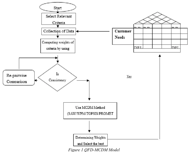
Figure 1 QFD-MCDM Model 2.2.2 Weighted Product Method (WPM)

This method is similar to simple additive weighting method. The main difference is multiplication is used instead of addition as shown below:

= ! "#$

Each normalized value of alternative with respect to attribute is raised to the power of relative weight corresponding attribute.

2.2.3 AHP steps

Some calculation steps are essential and explained as follows:

Establishing the hierarchical structure constructing the hierarchical structure with decision elements, decision-makers are requested to make pairwise comparisons between decision alternatives and criteria using a nine-point scale.

Calculating the consistency to ensure that the priority of elements is consistent, the maximum eigenvector or relative weights and max λ is calculated.

I.C. = (λmax – n)/(n-1) < 0.10 (1)

Where n is the number of components evaluated in the pairwise comparison matrix, and λmax is the largest eigen value characterizing the previous matrix. When the calculated CR values exceed the threshold, it is an indication of inconsistent judgment. In such cases, the decision makers would need to revise the original values in the pairwise comparison matrix. Finally, it is necessary to aggregate the relative priorities of the decision elements to obtain an overall rating for decision alternatives. The numerical analysis method is employed to calculate the eigen value vector and the maximized eigen value for an understanding of the consistency established and the relative weight among elements.

Constructing a fuzzy positive matrix a decision maker transforms the score of pair-wise comparison into linguistic variables via the positive triangular fuzzy number (PTFN).

2.2.4 TOPSIS Method

The method is first TOPSIS proposed by Hwang and Lin 1987. In general, TOPSIS has two main functions: one is to calculate the largest distance from the negative ideal solution; another alternative is to choose optimization which has the shortest distance from the ideal solution. In case of the decision problem analysis TOPSIS is an effective and practical method used for hierarchization by preference systems.

TOPSIS method was successfully applied to solve multi-criteria decision making problem in various industrial field. The model of multi-attribute decision making based on TOPSIS was organized for the elimination of logistics information technology decision problem. TOPSIS was used to manage competitive benchmarking in the product design process. TOPSIS integrated with other methods have been developed to handle multipurpose reactive power compensation problem. The method is described below:

Step 1: To determine the objective.

Step 2: Formation of matrix based decision table in which each row of the matrix is allocated to one alternative and each column to one attribute.

% = &11 ⋯ &1)⋮ ⋱ ⋮ & 1 ⋯ & )

Step 3: Calculate normalized matrix:

, =

-∑ .

Step 4: Decide the relative weights(wij) of attributes.

Step 5: Find weighted normalized matrix Vij

/ = ,

Step 6: Find the best positive idea and worst negative ideal. V +_{= max{V}

1 +, V2 +,……… Vj+} j=1,2…….n. V -_{= min{V}

1-, V2 -,……… Vj-} j=1,2…….n.

Step 7: Develop the distances between each alternative. The distances of each alternative from ideal solution can be calculated by the equation given below:

0_{= 1 / − /}0 . 3

4_{= 1 / − /}4 . 3

Step 8: Find the closeness of alternatives

& =_{5 0+}4 ₄₇

Rank the alternatives the preference order can be find in step 8, which is close to the ideal solution and far from the negative ideal solution. Recommend the best alternative. The preferred alternative is the one with the maximum value of Ci.

2.2.5 PROMETHEE Method:

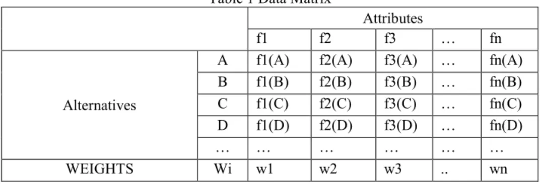
Step 1: Creating the Data Matrix: w = (w1, w2, ..., wn) k by c with weight = (f1, f2, ..., fn) to the alternative being considered by = (a, b, c, ...) for data matrix.

Table 1 Data Matrix

Attributes

f1 f2 f3 … fn

Alternatives

A f1(A) f2(A) f3(A) … fn(A) B f1(B) f2(B) f3(B) … fn(B) C f1(C) f2(C) f3(C) … fn(C) D f1(D) f2(D) f3(D) … fn(D)

… … … …

WEIGHTS Wi w1 w2 w3 .. wn

Step 2: Identification of preferred function Criteria: Six different preference function (Usual, U Type, V Type, Level type, Linear Type) is used for implementation.

Step 3: Determination of Preference Function:

Pa = :0 , f5a7 ≤ f5b7_{p[f5a7 − F5b7 , f5a7 > f5b7}

Step 4: Determine the preferred index: the choice of the Common functions can be determined reference index for each pair of alternatives. W (i = 1, 2, ... k) evaluated by weight by having a k and b the alternative preferred index are calculated by equation.

π5a, b7 =∑ w ∗ p 5a, b7 G

∑ wG

Step 5: Positive (ϕ+) and Negative (ϕ-) Superiority alternative rule for determining:

∅0_{5a7 =} 1

n − 1 π5a, b7 ∅4_{5a7 =} 1

n − 1 π5b, a7

Step 6: Determination of PROMETHEE I Partial Priority for Alternatives: In some cases are involved in the determination of the two alternatives A and B for partial priority.

Condition 1. If either of the conditions, a preferable alternative to the alternative b.

∅0_{5a7 > ∅}0_{5b7 and ∅}4_{5a7 < ∅}4_5b7

∅0_{5a7 > ∅}0_{5b7 and ∅}4_{5a7 = ∅}4_5b7

∅0_{5a7 = ∅}0_{5b7 and ∅}4_{5a7 < ∅}4_5b7

Condition 2. If the condition does not allow the following, A and B alternative is identical.

∅0_{5a7 = ∅}0_{5b7 and ∅}4_{5a7 = ∅}4_5b7

Condition3. If either of the following conditions A alternative, comparable to the B alternative.

∅0_{5a7 > ∅}0_{5b7 and ∅}4_{5a7 > ∅}4_5b7

∅0_{5a7 < ∅}0_{5b7 and ∅}4_{5a7 < ∅}4_5b7

Step 7: PROMETHEE II complete with identification of priorities for alternatives: The following equation is calculated with the help of exactly the priorities for each alternative. A calculated value of all alternatives with full priority ranking is determined by assessing precisely the same plane.

∅5a7 = ∅0_{5a7 − ∅}4_5a7

Depending on the exact priority value calculated for A and B are two alternative decisions are given below. If (a) > (b), A Alternative is superior.

If (a) = (b), A and B are identical alternatives. 3. Example

An example is considered to demonstrate the methodology of selection of bike. 3.1 AHP Analysis

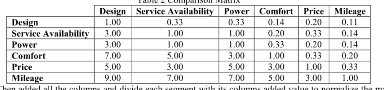
In survey on these aspects we gave some weight factors according to high or low numbers. The weight factor is an odd number series from 1 to 3,5,7,9 if it’s high and 1 to1/3, 1/5, 1/7, 1/9 if it’s low. By doing this we will get a comparison matrix.

Table 2 Comparison Matrix

Design Service Availability Power Comfort Price Mileage

Design 1.00 0.33 0.33 0.14 0.20 0.11 Service Availability 3.00 1.00 1.00 0.20 0.33 0.14 Power 3.00 1.00 1.00 0.33 0.20 0.14 Comfort 7.00 5.00 3.00 1.00 0.33 0.20 Price 5.00 3.00 5.00 3.00 1.00 0.33 Mileage 9.00 7.00 7.00 5.00 3.00 1.00

Then added all the columns and divide each segment with its columns added value to normalize the matrix and this process is called as normalizing the matrix.

Table 3 Normalized Matrix Design Service

Availability

Power Comfort Price Mileage

Design 0.04 0.02 0.02 0.01 0.04 0.06 Service Availability 0.11 0.06 0.06 0.02 0.07 0.07 Power 0.11 0.06 0.06 0.03 0.04 0.07 Comfort 0.25 0.29 0.17 0.10 0.07 0.10 Price 0.18 0.17 0.29 0.31 0.20 0.17 Mileage 0.32 0.40 0.40 0.52 0.59 0.52

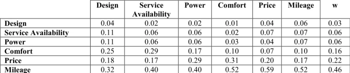
Now taking average of each row to get the high weight value and this matrix is called as weight factor matrix Table 4 Weighted factor Matrix

Design Service Availability

Power Comfort Price Mileage w

Design 0.04 0.02 0.02 0.01 0.04 0.06 0.03 Service Availability 0.11 0.06 0.06 0.02 0.07 0.07 0.06 Power 0.11 0.06 0.06 0.03 0.04 0.07 0.06 Comfort 0.25 0.29 0.17 0.10 0.07 0.10 0.16 Price 0.18 0.17 0.29 0.31 0.20 0.17 0.22 Mileage 0.32 0.40 0.40 0.52 0.59 0.52 0.46

Now we can see in above table that “Mileage” is the highest weight value about 0.46 but now to check that is our answer is consistent or not. For that we will do a consistency check.

For consistency we need a weight sum vector named as “Ws”, which is a multiplication of comparison matrix and weight factor matrix.

Table 5 Weight sum vector Ws 0.19 0.39 0.38 1.05 1.52 3.10

Now, Taking average of the “Ws dot 1/w” matrix which is 6.42 and this value called as element of consis and shown by λ.

Table 6 Dot product of weight some factor and inverse of weight factor matrix.

Ws 1/w Ws dot 1/w 0.19 32.26 6.17 0.39 15.67 6.12 0.38 16.20 6.20 1.05 6.10 6.40 1.52 4.54 6.91 3.10 2.18 6.74

To get consistency index, this formula is applied

&L)MNMOP)QRS)TPU5&S7 =V − )_{) − 1}

Where n is the no of alternatives and here we have 6 aspects or alternatives.

So the CI is 0.08and to get the consistency ratio we have to divide the CI by random index “RI” which depends on number of alternatives.

Table 7 Random Index

N 1 2 3 4 5 6 7 8 9 10

RI 0 0 0.58 0.9 1.2 1.24 1.32 1.41 1.45 1.49

Here for 6 alternatives the value of Random index would be 1.25. So The Consistency Ratio “CR” is 0.07.

The best consistency ratio would be if it’s less than 0.1 and when it goes equal or higher then it mean the comparison should be rechecked.

Now we got that Average is the aspects which have higher weight value.

Now the same AHP process would be followed for these three chosen bike models for each alternative. So for each alternative we have one weight factor matrix.

By multiplying all six weight factor matrix with the weight factor matrix from the main comparison matrix. Table 8 Wait matrix multiplication

Design Service Availability

Power Comfort Price Mileage w

TVS Star City 0.11 0.19 0.11 0.11 0.48 0.41 0.03 Mahindra Centuro 0.26 0.08 0.26 0.26 0.41 0.48 0.06 Honda Livo 0.63 0.72 0.63 0.63 0.11 0.11 0.06 0.16 0.22 0.46 3.2 SAW Method

Using the above weights the performance score for each attribute is calculated using normalized data.

= ∑ _∑ P1 = (0.11×0.03) + (0.19×0.06) + (0.11×0.06) + (0.11×0.16) + (0.48×0.22) + (0.41×0.46) P2= (0.26×0.03) + (0.08×0.06) + (0.26×0.06) + (0.26×0.16) + (0.41×0.22) + (0.48×0.46) P3 = (0.63×0.03) + (0.72×0.06) + (0.63×0.06) + (0.63×0.16) + (0.11×0.22) + (0.11×0.46) P1 = 0.3331 P2 = 0.3808 P3 = 0.2755 Ranking- 2-1-3

SAW suggested Bike-B as first choice, Bike-A as second choice, Bike-C as third choice. 3.3 WPM Method

The performance score for bike selection is calculated using same normalized data and weights of attributes using equation:

= ! "#$ The values of Pi are:

P1 = 0.110.03 × 0.190.06 × 0.110.06 × 0.110.16 × 0.480.22 × 0.410.46 P2= 0.260.03 _{× 0.08}0.06 _{× 0.26}0.06 _{× 0.26}0.16 _{× 0.41}0.22 _{× 0.48}0.46 P3 = 0.630.03 × 0.720.06 × 0.630.06 × 0.630.16 × 0.110.22 × 0.110.46 P1 = 0.2943 P2 = 0.3598 P3 = 0.1947 Ranking- 2-1-3

WPM suggested Bike-B as first choice, Bike-A as second choice, Bike-C as third choice. 3.4 TOPSIS analysis

Table 9 Normalized date of example Attributes

Alternatives

Design Service Availability

Power Comfort Price Mileage

Bike-A .11 .19 .11 .11 .48 .41

Bike-B .26 .08 .26 .26 .41 .48

Bike-C .63 .72 .63 .63 .11 .11

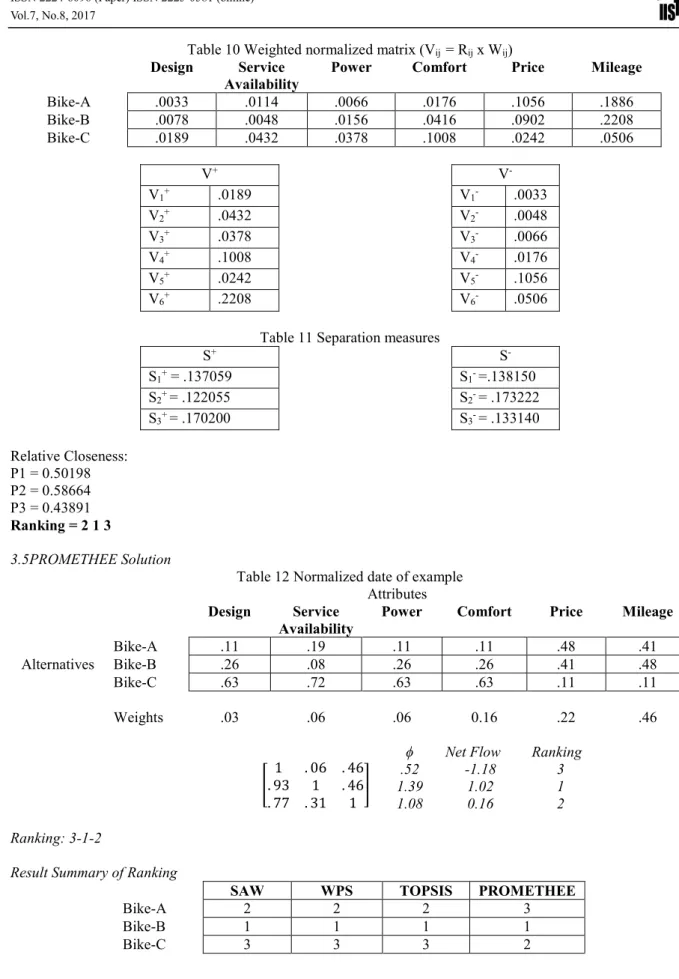
Table 10 Weighted normalized matrix (Vij = Rij x Wij)

Design Service Availability

Power Comfort Price Mileage

Bike-A .0033 .0114 .0066 .0176 .1056 .1886 Bike-B .0078 .0048 .0156 .0416 .0902 .2208 Bike-C .0189 .0432 .0378 .1008 .0242 .0506 V+ _V -V1+ .0189 V1- .0033 V2+ .0432 V2- .0048 V3+ .0378 V3- .0066 V4+ .1008 V4- .0176 V5+ .0242 V5- .1056 V6+ .2208 V6- .0506

Table 11 Separation measures

S+ _S -S1+ = .137059 S1- =.138150 S2+ = .122055 S2- = .173222 S3+ = .170200 S3- = .133140 Relative Closeness: P1 = 0.50198 P2 = 0.58664 P3 = 0.43891 Ranking = 2 1 3 3.5PROMETHEE Solution

Table 12 Normalized date of example Attributes

Alternatives

Design Service Availability

Power Comfort Price Mileage

Bike-A .11 .19 .11 .11 .48 .41

Bike-B .26 .08 .26 .26 .41 .48

Bike-C .63 .72 .63 .63 .11 .11

Weights .03 .06 .06 0.16 .22 .46

ϕ Net Flow Ranking

1 . 06 . 46 . 93 1 . 46 . 77 . 31 1 .52 1.39 1.08 -1.18 1.02 0.16 3 1 2 Ranking: 3-1-2

Result Summary of Ranking

SAW WPS TOPSIS PROMETHEE

Bike-A 2 2 2 3

Bike-B 1 1 1 1

Bike-C 3 3 3 2

4.Conclusions

The proposed analysis model has practical application as Bike Section problem shown further more proposed method is also used to solve other optimization problems in many industries. A Methodology based on QFD with optimization tools (AHP, TOPSIS, and PROMETHEE) is suggested for product design and development in

manufacturing industry, which helps in selection of suitable customer needs among large numbers. This approach can also useful to select key column in each phase of QFD and provides best solution for each situation. The method allows assigning values of relative importance to the criterion based on customer preference. Developed models have been proven to allocate weights per demand for the first phase of QFD. These models can be applied to each QFD phase in order to analyze product quality of different industries.

The decision making tools of other criteria can be used for the measurement of product quality and the impact of the developed models can be analyzed. The future direction of a theoretical study is analyzing the similarities and differences between AHP, TOPSIS, PROMETHEE and other MCDA / MCDM methods.

References

1. Afshari A., Mojahed M., Yusuff, R. M. (2010), “Simple Additive Weighting approach to Personnel Selection problem”, International Journal of Innovation, Management and Technology, vol. 1, no. 5, pp.511–515. 2. Akao, Y. (1990), Introduction to Quality Deployment (Application Manual of Quality Function Deployment

(1), (Japanese) JUSE Press.

3. Akao, Y.(1972), New Product Development and Quality Assurance – Quality Deployment Sys-tem,(Japanese)Standardization and Quality Control. Vol. 25, No. 4, pp. 7-14.

4. Baky, I. & Abo-Sinna, M. A. (2013), TOPSIS for bi-level MODM problems. Applied Mathematical Modelling, 37, 1004–1015.

5. Bansal, P. Kumar(2013), 3PL selection using hybrid model of AHP-PROMETHEE, IJS & OM, 14 373-397. 6. Bilbao-Terol, A., Arenas-Parra, M., Canal-Fernandez, V., & Antomil-Ibias, J. (2014). Using TOPSIS for

assessing the sustainability of government bond funds. Omega, 49, 1–17.

7. Brans, J.P. and Mareschal, B. (1995), The PROMETHEE VI procedure. How to differentiate hard from soft multicriteria problems. Journal of Decision Systems, 4:213–223.

8. Brans, J.P. Vincke H., (1982), A preference ranking organization method: The PROMETHEE method, MS, 31 647–656.

9. Brans, J.P., P. Vincke H., Mareschall B., (1986), How to select and how to rank projects: The PROMETHEE method, EJOR, 14 228-238.

10. Carlsson C., Fuller R.,( 1996), “Fuzzy multiple criteria decision making: Recent developments”, Fuzzy Sets and Systems, vol. 78, pp.139-153.

11. Chan JWK, Tong TKL. Multi-criteria material selections and end-of-life product strategy: a grey relational approach. Mater Des 2007;28:1539–46.

12. Cheng, J. H., Lee, C. M., & Tang, C. H. (2009), An application of fuzzy Delphi and fuzzy AHP on evaluating wafer supplier in semiconductor industry. WSEAS Transactions on Information Science and Applications, 6(5), 756-767.

13. Churchman C. W., Ackoff R. L., Arnoff E. L.,( 1957), “Introduction to Operations Research”, Wiley. New York.

14. Cohen, L., (1995), Quality function deployment: how to make QFD work for you. Addison-Wesley Publishing Company. United States of America.

15. Fishburn PC (1967), Additive utilities with incomplete product set: applications to priorities and assignments. Operations Research Society of America, Baltimore.

16. French, S., Simpsom, L., Atherton, E., Belton, V., Dawes, R., Edwards, W. , Hamalainen, R.P., Larichev, O.I., Lootsma, F.A., Perman, A. and Vlek, C. (1998), Problem formulation for Journal of Multi-Criteria Decision Analysis : report of a workshop. Journal of Multi-Criteria Decision Analysis, 7(5):242-262. 17. Garcia-Cascales, M. S., & Lamata, M. T. (2012), On rank reversal and TOPSIS method. Mathematical and

Computer Modelling, 56, 123–132.

18. Han S.B., Chen S.K., Ebrahimpour M., Sodhi M.S. (2001), A conceptual QFD planning model. International Journal of Quality & Reliability Management, Vol. 18, No. 8, pp. 796 – 812.

19. Jadidi, O., Hong, T. S., & Firouzi, F. (2009), TOPSIS extension for multi-objective supplier selection problem under price breaks. International Journal of Management Science and Engineering Management, 4, 217–229. 20. Jahanshahloo, G. R., Khodabakhshi, M., Hosseinzadeh Lotfi, F., & Moazami Goudarzi, M. (2011), A

cross-efficiency model based on super-cross-efficiency for ranking units through the TOPSIS approach and its extension to the interval case. Mathematical and Computer Modelling, 53.

21. Jiang, J. C., Shiu, M. L., & Tu, M. H. (2007), Quality function deployment (QFD) technology designed for contract manufacturing. The TQM Magazine, 19(4), 291-307.

22. Karimi-Nasab, M., & Seyedhoseini, S. M. (2013), Multi-level lot sizing and job shop scheduling with compressible process times: A cutting plane approach. European Journal of Operational Research, 231, 598– 616. doi:10.1016/j.ejor.2013.06.021.

23. Khademi-Zare, H., Zarei, M., Sadeghieh, A. and Saleh Owlia, M.(2010), Ranking the strategic actions of Iran mobile cellular telecommunication using two models of fuzzy QFD, Telecommunications Policy, vol. 34, no.

11, pp. 747–759.

24. Kou, G., Peng, Y., & Lu, C. (2014), MCDM approach to evaluating bank loan default models. Technological and Economic Development of Economy, 20, 292–311.

25. Kwong, C.K., Bai, H.,( 2002), A fuzzy AHP approach to the determination of importance weights of customer requirements in quality function deployment. Journal of Intelligent Manufacturing, Vol. 13, No. 5, pp. 367– 377.

26. Lootsma, F.A. (2000), Distributed multi-criteria decision making and the role of the participants in the process. Journal of Multi-Criteria Decision Analysis, 9(1-3):45-55.

27. Mahmoodzadeh, S., Shahrabi, J. , Pariazar, M. and Zaeri, M. S.( 2007), “Project selection by using fuzzy AHP and TOPSIS technique,” International Journal of Human and Social Sciences, vol. 1, no. 3, pp. 135–140. 28. Miller DW, Starr MK (1969) Executive decisions with operations research. Prentice Hall, Englewood Cliffs,

New Jersey.

29. Gunasekaran, N. Rathesh, S., Arunachalam S., and Koh S. C. L.,( 2006), “Optimizing supply chain management using fuzzy approach,” Journal of Manufacturing Technology Management, vol. 17, no. 6, pp. 737–749.

30. Pohekar S. D., Ramachandran, M.( 2004), “Application of multi-criteria decision making to sustainable energy planning—A review”, Renewable and Sustainable Energy Reviews, vol.8, no. 4, pp.365–381. 31. Ramanathan, L.S. Ganesh (1995), Using AHP for resource allocation problems, European Journal of

Operational Research 80 (2) 410–417.

32. Rao RV. A material selection model using graph theory and matrix approach. Mater Sci Eng A 2006;431:248– 55.

33. Saaty, T. (1988), What is the analytic hierarchy process? In G. Mitra, H. Greenberg, F. Lootsma, M. Rijkaert, & H. Zimmermann (Eds.), Mathematical Models for Decision Support 48 (pp. 109–121). Berlin: Springer. 34. Saaty, T. L. (1971), On polynomials and crossing numbers of complete graphs. Journal of Combinatorial

Theory, Series A, 10, 183–184.

35. Saaty, T. L. (1980), The analytic hierarchy process: Planning, priority setting, resources allocation. New York, NY: McGraw.

36. Saaty, T. L. (1980). The analytic hierarchy process: Planning, priority setting, resources allocation. New York, NY: McGraw.

37. Saaty, T. L. (1996). Decision making with dependence and feedback: the analytic network process: The organization and prioritization of complexity. Pittsburgh: Rws Publications.

38. Shanian A, Savadogo O. (2006), TOPSIS multiple-criteria decision support analysis for material selection of metallic bipolar plates for polymer electrolyte fuel cell. J Power Sour; 159:1095–104.

39. Triantaphyllou E. (2000), Multi-criteria decision making methods: a comparative study. London: Springer-Verlag.

40. Zhang, H. & Yu, L.(2012), MADM method based on cross-entropy and extended TOPSIS with interval-valued intuitionistic fuzzy sets. Knowledge-Based Systems, 30, 115–120.

41. Zhang, Y., Sun, Y., & Qin, J. (2012), Sustainable development of coal cities in Heilongjiang province based on AHP method. International Journal of Mining Science and Technology, 22, 133–137.